Article

Reducing Statistical Uncertainty in Elastic Settlement Analysis of Shallow Foundations Relying on Targeted Field Investigation: A Random Field Approach

by
Panagiotis Christodoulou
and
Lysandros Pantelidis
*
Department of Civil Engineering and Geomatics, Cyprus University of Technology, 2-8 Saripolou st, 3036 Limassol, Cyprus
*
Author to whom correspondence should be addressed.
Geosciences 2020, 10(1), 20; https://doi.org/10.3390/geosciences10010020
Submission received: 13 November 2019 / Revised: 23 December 2019 / Accepted: 26 December 2019 / Published: 1 January 2020

Abstract

:
The present paper deals with the practical problem of reducing statistical uncertainty in elastic settlement analysis of shallow foundations by relying on targeted field investigation with the aim of an optimal design. In a targeted field investigation, the optimal number and location of sampling points are known a priori. As samples are taken from the material field (i.e., the ground), which simultaneously is a stress field (stresses caused by the footing), the coexistence of these two fields allows for some points in the ground to better characterize the serviceability state of structure. These points are identified herein through an extensive parametric analysis of the factors controlling the magnitude of settlement; the number of different cases considered was 3318. This is done in an advanced probabilistic framework using the Random Finite Element Method (RFEM) properly considering sampling of soil property values. In this respect, the open source RSETL2D program, which combines elastic finite element analysis with the theory of random fields, has been modified as to include the function of sampling of soil property values from the generated random fields and return the failure probability of footing against excessive settlement. Two sampling strategies are examined: (a) sampling from a single point and (b) sampling a domain (the latter refers to e.g., continuous cone penetration test data). As is shown in this work, by adopting the proper sampling strategy (defined by the number and location of sampling points), the statistical error can be significantly reduced. The error is quantified by the difference in the probability of failure comparing different sampling scenarios. Finally, from the present analysis, it is inferred that the benefit from a targeted field investigation is much greater as compared to the benefit from the use of characteristic values in a limit state design framework.

1. Introduction

Unlike the variability of manufactured materials used in structures, geotechnical variability is a complex attribute that results from many disparate sources of uncertainties [1]. The three primary sources are: (a) inherent variability, (b) statistical uncertainty and (c) systematic uncertainties [2,3]. Inherent variability results from the fact that, even in seemingly homogenous soil media, the soil properties exhibit variability by nature. Statistical uncertainty is attributed to limited soil testing. The systematic uncertainties stem from the discrepancies between the laboratory and in situ conditions, due to factors such as scale, anisotropy and water saturation.
The statistical uncertainty in geotechnical engineering has been studied only by a few researchers so far. In this respect, Jaksa et al. [4] investigated the effect of soil variability and site investigation scope on the settlement of a footing of a three story building, and observed that the likelihood of under-designing or over-designing a footing decreases as the scope of the investigation increases. Griffiths et al. [5] studied the effect of sampling on the reliability of passive earth pressure by using the Random Finite Element Method (RFEM). Considering a limited number of sampling locations (four in number), they concluded that a single sampling point located at a horizontal distance equal to approximately one wall height from the wall, results in a lower probability of failure independent of the scale of fluctuation, and that the inclusion of additional sample points to characterize the soil properties reduces the probability of failure. Yang et al. [6] used conditional random fields, enabling the site investigation data to be incorporated directly in probabilistic analysis. They found that the coefficient of variation of factor of safety can be reduced by incorporating more site investigation data. Ching and Phoon [7] addressed the statistical uncertainties associated with the estimation of a depth-dependent trend function and spatial variation about the trend function using limited site-specific geotechnical data. This study proposed a two-step approach to characterize the uncertainties in all parameters, including the functional form of the trend, within a consistent Bayesian framework. Yang et al. [8] studied the importance of sampling location on slope stability assessment based on statistical hypothesis testing concluding that the slope crest is the optimal location to conduct geotechnical site exploration. Fenton et al. [9] studied the effect of number of samples and type of trend removal on residual uncertainty. They found that removing the sample mean outperforms removing the best linear unbiased estimate (BLUE) when the actual field scale of fluctuation is small, but the BLUE is better to use if the actual scale of fluctuation is large relative to the domain size. Also, they found that more samples reduce the uncertainty when the field scale of fluctuation is small, but does not have much impact when the field scale of fluctuation is large. Li et al. [10] linked 3D conditional random fields with finite elements, within a Monte Carlo framework, to investigate optimum sampling locations and the cost-effective design of a slope. Their results clearly demonstrate the potential of 3D conditional simulation in directing exploration programs and designing cost saving structures. More recently, Li et al. [11] examined the influence of soil strength mean, standard deviation and scale of fluctuation on the risk of slope design failure for different levels of site investigation scope using conditional random fields. They found that there is an optimal number of site investigation tests, beyond which the cost of additional boreholes does not justify the cost savings due to reduced slope failure risk. Finally, the authors [12] studied the effect of targeted field investigation on the reliability of earth retaining structures in the active state by working with the Random Finite Element Method. This extensive parametric analysis involving 2165 different cases (for each mode of failure, i.e., sliding and translational) showed that the optimal horizontal sampling location in the active state is adjacent to the wall face, whilst the optimal sampling domain length is equal to the wall height.
Regarding the various design codes (e.g., EN 1997-2 [13] and AASHTO [14]), these are limited to some general recommendations (see Appendix A), focusing mainly on the extent of the subsurface exploration and aiming at identifying possible unfavorable geological conditions.
The present paper deals with the practical problem of reducing statistical uncertainty in the elastic settlement analysis of shallow foundations by relying on targeted field investigation with the aim of an optimal design. In a targeted field investigation, the optimal number and location of sampling points are known a priori. As samples are taken from a material field (i.e., the ground; see Figure 1), which is simultaneously a stress field (stresses caused by the footing), the coexistence of these two fields, logically thinking, allows for some points in the ground to better characterize the serviceability state of structure. If this assumption is valid, then the soil property values sampled from specific location(s) would result systematically to lower probabilities of failure. These points are identified herein through an extensive parametric analysis of the factors controlling the magnitude of settlement. This is done in an advanced probabilistic framework using the Random Finite Element Method (RFEM) [15] properly considering sampling of soil property values. In this respect, the open source RSETL2D program, which combines elastic finite element analysis with the theory of random fields, has been modified as to include the function of sampling of soil property values from the generated random fields and return the failure probability of footing against excessive settlement. Contrary to the common belief that statistical uncertainty decreases with increasing number of samples e.g., [16,17,18,19], the present analysis will show that the statistical error in an elastic settlement analysis can be effectively minimized only when targeted field investigation is carried out.

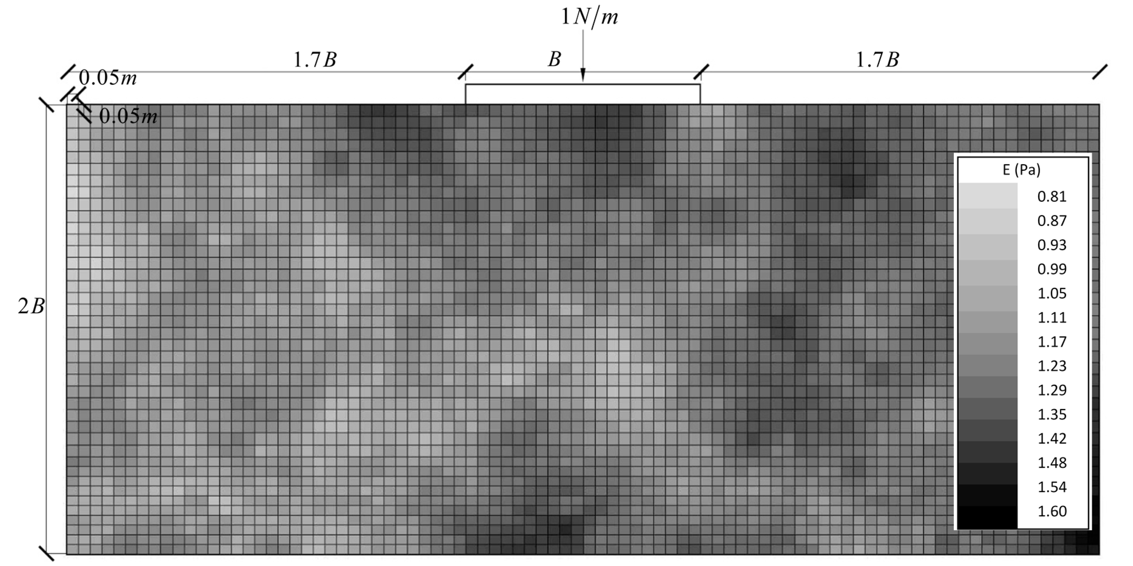
2. Two-Dimensional Probabilistic Elastic Settlement Analysis Based on the Random Finite Element Method (RFEM)

As mentioned, the present analysis was based on the open source RSETL2D program ([20]). The program involves the generation and mapping of the elastic modulus of soil (E; which is treated as random field) onto a finite element mesh using the local average subdivision method [21], taking into account the element size in the local averaging process. The random field of E is fully described by its mean, standard deviation, scale of fluctuation and spatial correlation function. The scale of fluctuation, θ, (also known as spatial correlation length) is defined as the distance within which the soil property shows a relatively strong correlation or persistence from point to point [22]. The RSETL2D program calculates the settlement induced by a single strip footing (or a pair of strip footings) founded on a soil having spatially random E; the RSETL2D program can return the settlement induced at any finite element node; however, in the parametric analysis that follows, the settlement is calculated at the center of the footing. The procedure is repeated m times; m is the number of realizations, where each RFEM realization refers to a new random field of E.
The footing(s) is (are) assumed to be founded on a soil layer underlain by bedrock. The physical problem is represented using a two-dimensional (plane-strain) model as shown in Figure 1. The soil mass is discretized into 4-noded quadrilateral elements. The nodes along the left and right boundary of the finite-element model are constrained against horizontal displacement but are free to slide vertically, while the nodes on the horizontal boundary are fixed. The footing(s) is (are) assumed to be rough and rigid, undergoing no rotation. A unit force P (per unit length in the out-of-plane direction) is applied to each footing—since elastic settlement is directly proportional to P.
For the needs of the present research, the original RSETL2D program has been extended by the authors as to:
  • Virtually sample elastic modulus values from the random field generated in each RFEM realization,
  • Calculate the footing settlement (again in each RFEM realization) considerring that the soil is homogenous, having E equal to the mean of the values sampled (this settlement is calculated in addition to the settlement of footing lying on spatially random soil) and,
  • Estimate the failure probability of the footing.
The latter is defined by the fraction of the realizations resulted in failure over the total number of realizations. In each RFEM realization, “failure” is considered to have occurred when the “actual” settlement value, referring to the spatially random soil, is greater than the respective predicted value, referring to the spatially uniform soil. That is, it stands that
p f = P [ ρ a c t u a l > ρ p r e d i c t e d ] ,
where, the symbol ρ denotes footing settlement.
The modified program was validated as follows. First a given footing was solved using in the original RSETL2D program a deterministic soil modulus value. Then the same footing was solved with the modified program using values sampled from various points (because the same deterministic soil modulus value was spread out in the finite element mesh, all E values sampled were the same). The two programs gave exactly the same results, indicating that the sampling function was correctly embedded into the original program.

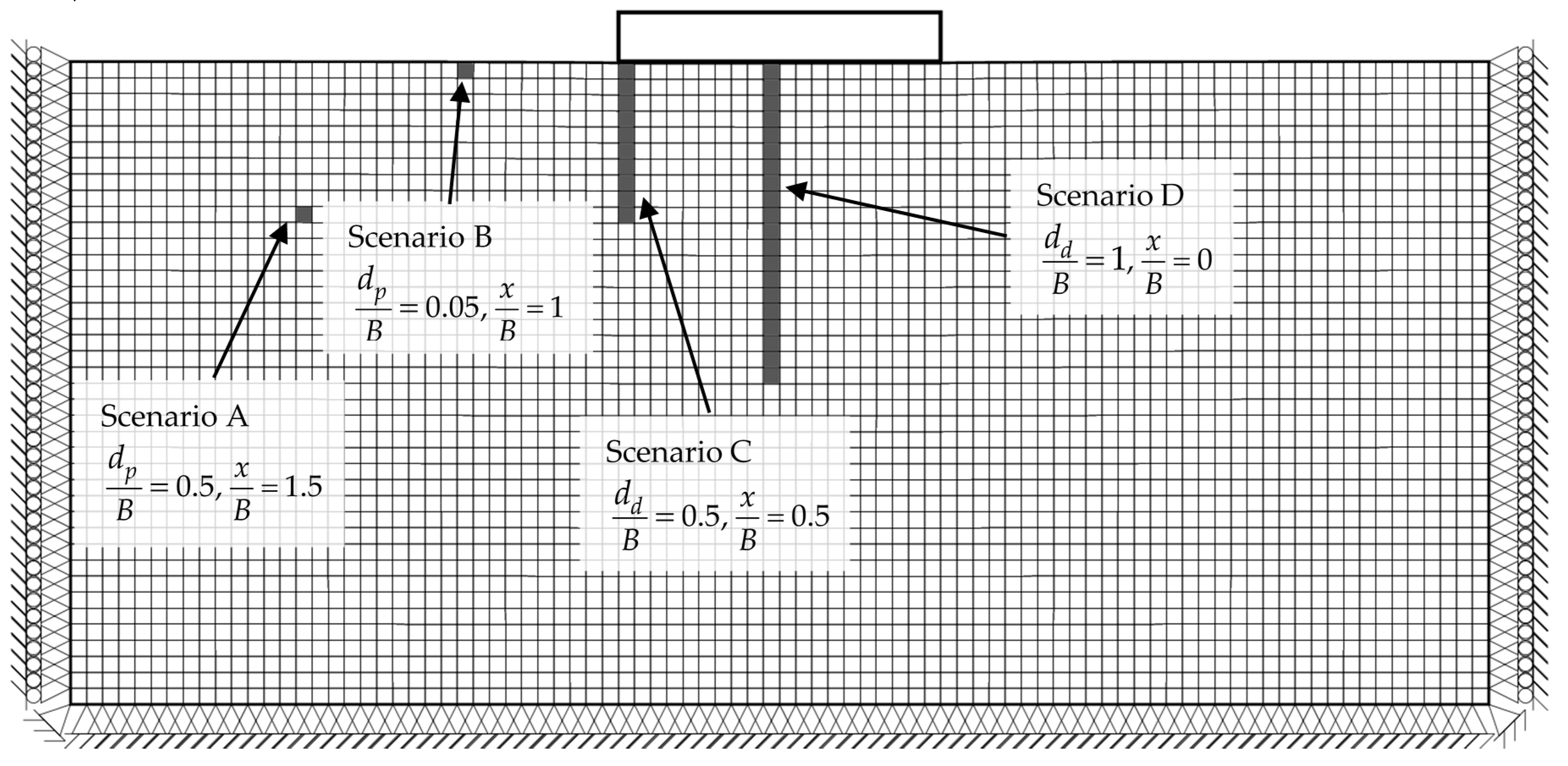
3. Parametric Study for Determining the Optimal Sampling Strategy

This paper deals with the case of a single strip footing (eccentrically loaded and interfering footings are currently under examination by the authors). Both the sampling from a single point and the sampling from an entire domain strategy are investigated through an extensive parametric analysis (3318 different cases) of the factors controlling the magnitude of settlement for defining the strategy that minimizes the probability of failure and thus, the statistical error (this strategy is called hereafter “optimal sampling strategy”). The “optimal sampling strategy” refers to the number of sampling points and their location resulting to an optimal design. The error is quantified comparing the probability of failure value obtained based on different sampling scenarios. The term “sampling”, in practice, may refer to either undisturbed specimens or continuous probing test data (e.g., cone penetration test).
In the finite element analysis that follows, the soil mass is discretized into a 88 (horizontal direction) by 40 (vertical direction) mesh, consisting of four-noded square elements having edge 0.05 m. The strip footing occupies width on the surface of the finite element mesh equal to 20 elements (i.e., B = 20 × 0.05 m = 1 m, called hereafter “reference footing”; other footing widths will also be considered in a later sections). A typical random field is shown in Figure 1. The effect of the distance between the edge of the footing and the respective lateral boundary was investigated prior to the analysis. As shown in Appendix B, the error inserted considering a 20-element footing centered on the surface of a 88-element mesh is negligible; that makes a free distance between each edge of footing and the respective lateral boundary equal to 1.7B. The same distance of 1.7B was kept the same for the other footing widths considered (i.e., B = 1,2 and 3 m); however, the element size for the B = 2 and 3 m footings was 0.1 m and 0.15 m, respectively.
In the present analysis, only E is treated as random field. According to Fenton and Griffiths [15], the Poisson’s ratio, ν, have a smaller relative spatial variability and only a second-order importance to settlement statistics. Generally, when not mentioned herein, ν = 0.25, whilst μ E = 1 Pa (E is assumed to follow a log-normal distribution [23,24]). Moreover, it is mentioned that the footing is subjected to a centrally applied vertical force of P = 1 N/m (unit force per unit length in the out-of-plane direction). A Markovian spatial correlation function has been adopted:
ρ ( τ ) = exp [ 2 τ / θ ] ,
where, τ is the absolute distance between two measurements [25,26].
Aiming at finding the optimal sampling strategy, the following parameters will be examined: the sampling depth ( d p ) and horizontal distance for the case of sampling from a single point (measured from the soil surface and the axis of strip footing respectively), the sampling length ( d d ) and horizontal distance of the continuous probing test location for the case of sampling an entire domain (measured as in the previous case), the scale of fluctuation of soil ( θ ) , the footing width ( B ) , the coefficient of variation (COV) of E of soil, the effect of the Poisson’s ratio (ν) value of soil and the anisotropy of soil mass ( θ h θ v ) . It is noted that the symbol θ without subscript denotes, hereafter, isotropic conditions ( θ h = θ v ) . Four sampling scenarios are indicatively shown in Figure 2 (scenarios A and B refer to a single sampling point, whilst scenarios C and D to continuous probing tests).
The optimal sampling point or domain will be identified by comparing the failure probability values ( p f ) derived from various sampling strategies. Apparently, when dealing with small differences in p f , the stability of the results is very important. In this respect, the number of realizations was set equal to 10,000; this number, as shown in Appendix B, can be considered adequate for the needs of the present analysis.

3.1. Sampling from a Single Point

3.1.1. Effect of Scale of Fluctuation

Example charts showing the variation of p f with respect to d p / B for various θ / B values are given in Figure 3. From the figure in question, it is inferred that the optimal sampling location lies at the center of strip foundation ( x / B = 0 ) and at a depth of approximately 0.7 B. It is also observed that as θ / B tends to zero, the p f value tends to a single value, that is, p f becomes independent of the sampling depth.
For drawing the curves in Figure 3, the soil mass was generally considered isotropic. However, due to natural deposition and soil formation processes, the soil often appears to be anisotropic. Indeed, according to the literature, the spatial variability of soil in the horizontal direction is roughly 9 to 13 times greater than the respective one in the vertical direction [27,28,29,30,31]. Driven from these findings, the effect of soil anisotropy on the optimal sampling location is investigated herein by comparing the θ h = θ v case with the θ h = 10 θ v case, i.e., the reference footing-soil system with θ v / B = θ h / B = 5 will be compared with a respective one having θ v / B = 5 and θ h / B = 50 . In this respect, the optimal sampling location was found not to be affected by soil anisotropy (see heavy bold line in Figure 3c).

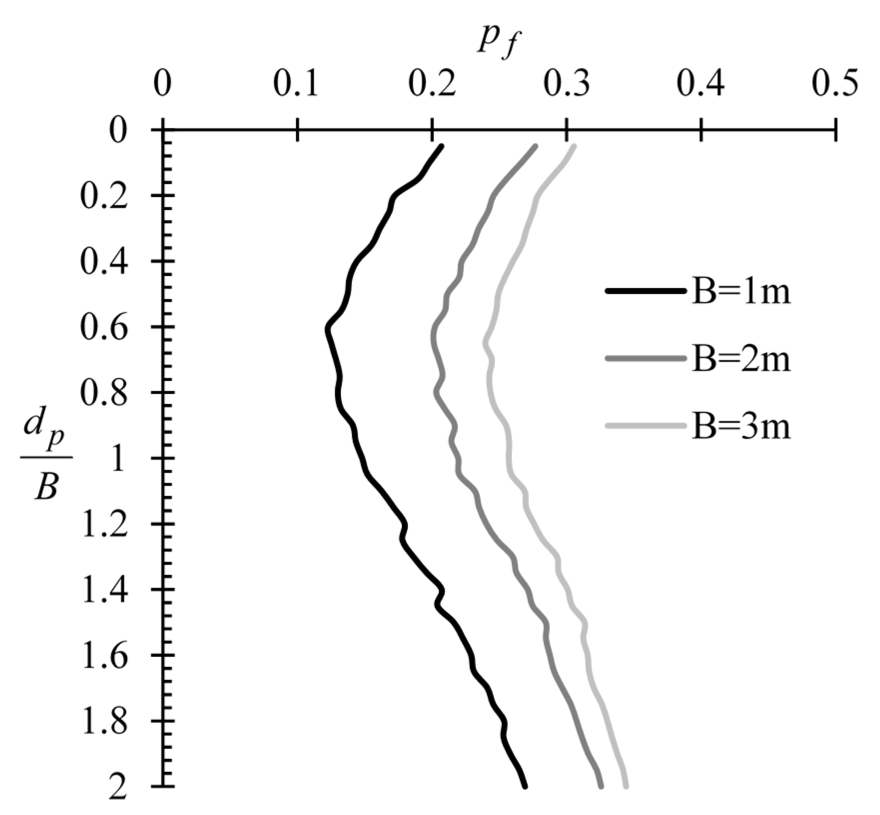
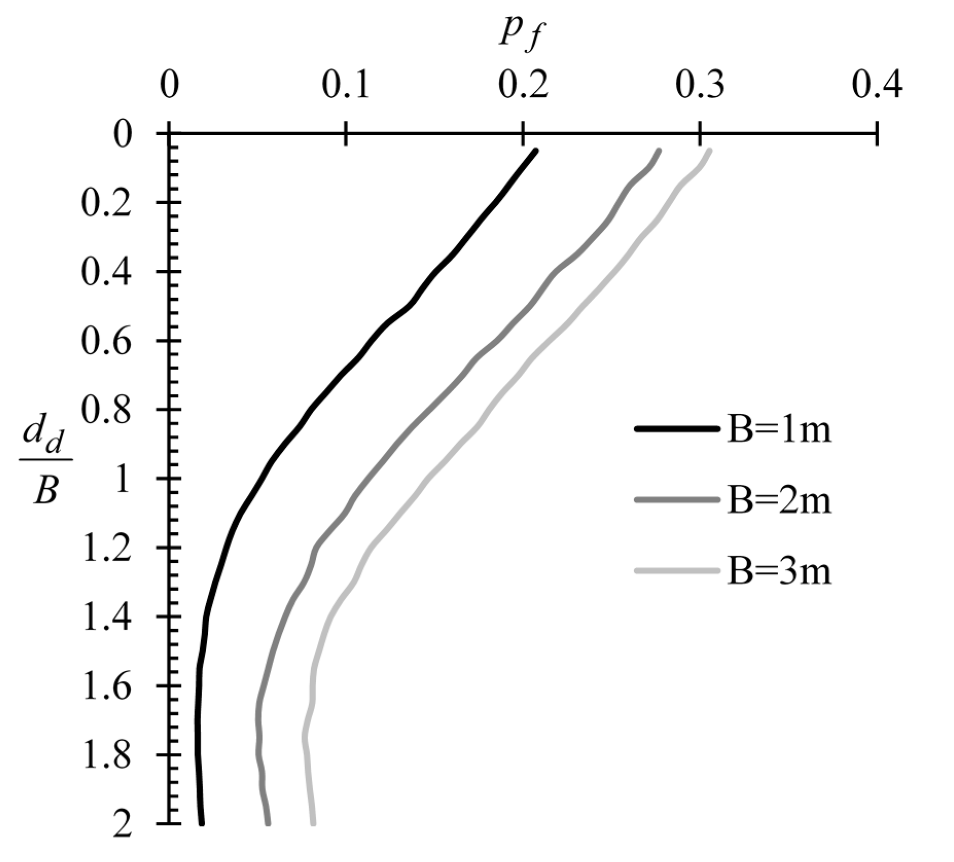
3.1.2. Effect of Footing Width (B)

The variation of p f with d p / B is shown in Figure 4 for three footing widths, i.e., B = 1, 2 and 3 m. The analysis showed that the optimal sampling depth is not affected by the footing width, whilst again the x / B = 0 case leads to the smaller statistical error. The curves in Figure 4 refer to x / B = 0.

3.1.3. Effect of COV of the Elastic Constants of Soil

Five COV values of soil modulus, E , were considered, namely, C O V = 0.1, 0.2, 0.3, 0.4 and 0.5. The analysis showed that the optimal sampling depth is independent of the COV of E, where again the smaller statistical error is found for x / B = 0. The five curves in Figure 5 refer to x / B = 0.

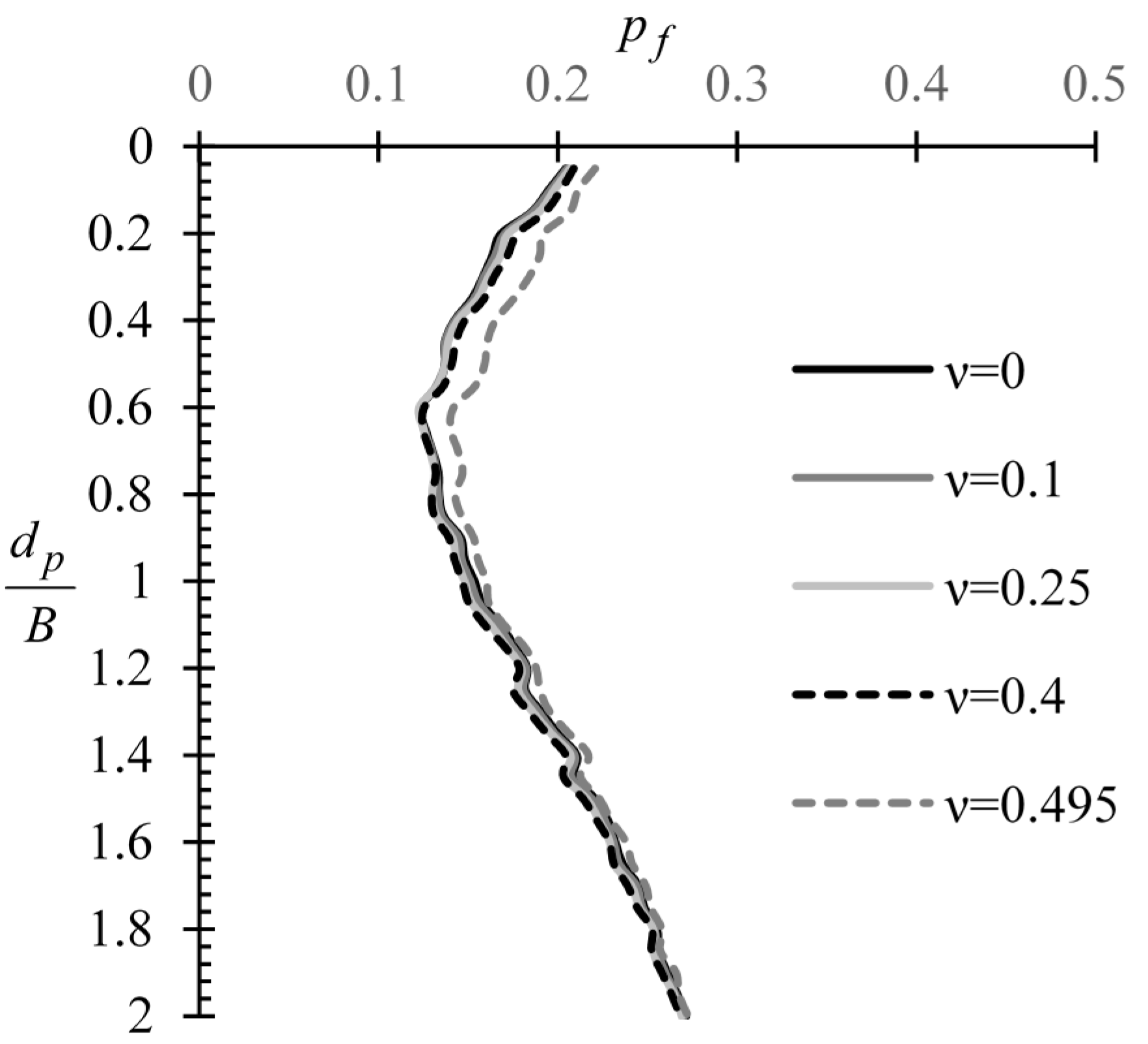
3.1.4. Effect of the Elastic Constant Values of Soil

For all cases considered above, the Poisson’s ratio of soil was equal to 0.25. Parametric study on the effect of the ν on the optimal sampling location, however, showed that the latter is not affected by the parameter in question. The following ν values were considered, i.e., ν = 0, 0.1, 0.25, 0.4 and 0.495. The five curves shown in Figure 6 refer to x / B = 0. Similarly to the Poisson’s ratio value, the optimal sampling location is not affected by the mean value of the elastic modulus of soil.

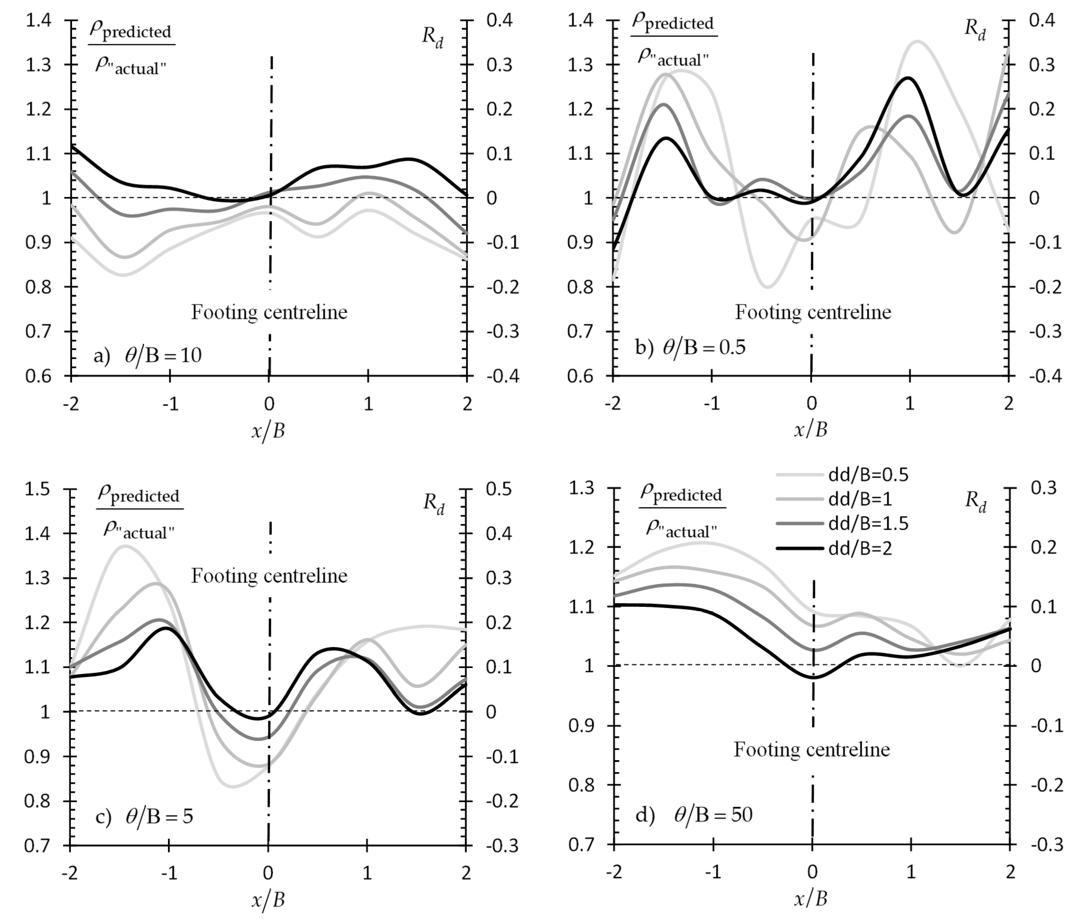
3.2. Sampling from an Entire Domain

This sampling strategy refers to data obtained from continuous probing tests, e.g., the cone penetration test (CPT) and the standard penetration test (SPT). In this respect, the elastic modulus of soil (E) derives indirectly through empirical correlations (e.g., [13,32,33,34]). In the present section, the length of the sampling domain is always measured from soil surface.
In the parametric analysis carried out, three footing widths were considered, i.e., B = 1, 2 and 3 m, whilst the distance between two successive sampling points (in the vertical direction) was B/20 for all cases. The maximum sampling domain length considered was always two times the footing width B. The arithmetic mean of the soil elastic modulus values sampled was used in the analysis. It is noted that for all cases examined, the optimal sampling distance was found again to be at x / B = 0. Thus, for economy of space, the analysis below generally refers to x / B = 0.

3.2.1. Effect of Scale of Fluctuation

Example charts showing the variation of p f with respect to d d / B for various θ / B and x / B values are provided in Figure 7. From this figure, it is inferred that the optimal horizontal sampling distance from the footing center for every θ / B value is again for x / B = 0. It is also observed that the required domain length is smaller for greater θ values of soil. Given now that the soil samples will be taken from x / B = 0, it is advisable that a domain length of at least 2B must be considered. This practice may significantly reduce the statistical error. The variation of p f with d d / B for the case of anisotropic soil mass ( θ v / B = 5 and θ h / B = 50 ) is shown in Figure 7c (heavy bold line). Generally, it can be said that the required sampling domain length was found to be somewhat smaller in comparison to the case of the isotropic soil mass.

3.2.2. Effect of Footing Width

In this paragraph three footing widths were considered, i.e., B = 1,2,3 m. Figure 8 presents the variation of p f with d d / B for these three cases. From this figure, it is clear that the footing width has only a minor influence on the required sampling domain length.

3.2.3. Effect of COV of the Elastic Constants of Soil

In this paragraph, five C O V values of E were considered, i.e., C O V = 0.1, 0.2, 0.3, 0.4 and 0.5. The optimal horizontal sampling distance from the footing center was found not to be affected by the C O V of E , whilst again the x / B = 0 case leads to the smaller probabilities of failure. Thus, only the x / B = 0 case will be presented here. From Figure 9 it is, generally, inferred that the C O V of E largely affects the optimal sampling domain length. More specifically, as the C O V of E increases the sampling domain length required to minimize the statistical error also increases.

3.2.4. Effect of the Elastic Constant Values of Soil

The variation of p f with respect to d d / B for different Poisson’s ratio (ν) values is shown is Figure 10; the optimal sampling distance was also found to be at x / B = 0 for any ν value, thus, only this case is presented in this paragraph. From Figure 10, it is obvious that the Poisson’s ratio value has no effect on the optimal sampling domain length. The same stands for the mean value of the elastic modulus of soil.

4. Discussion

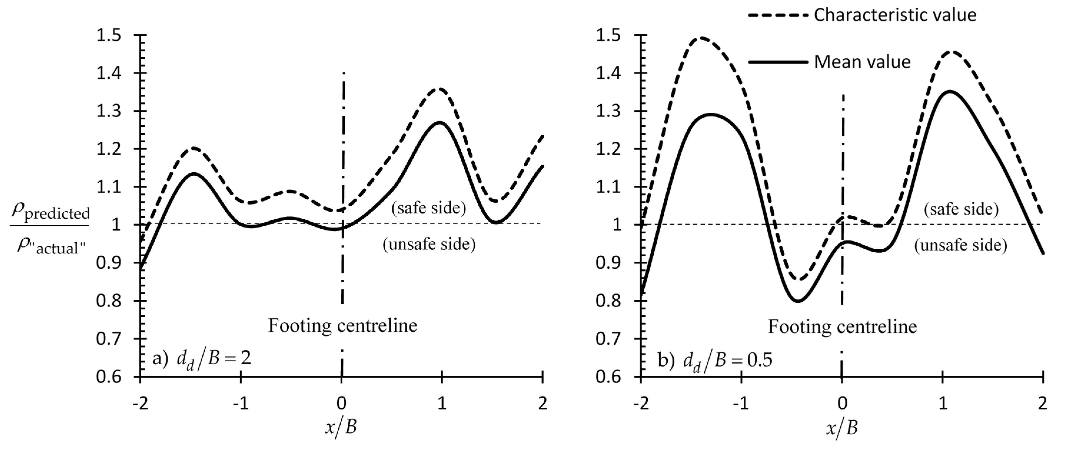
4.1. The Importance of Targeted Field Investigation in Practice

The importance of targeted field investigation, where samples are taken from a priory known optimal locations, is highlighted here. A random elastic modulus field referring to a specific RFEM realization (such as those presented in Figure 1, Figure 11, Figure 12 and Figure 13, it can be said that it convincingly represents a real field. In the four examples presented below, the footing and the mesh/boundary conditions are the same as those presented in Section 3 (i.e., the reference footing). The material properties (i.e., the elastic constant values of the soil) are given in Table 1. The four examples, in essence, differ in the scale of fluctuation, since as shown in the present research, the mean and C O V values of E have no effect on the optimal sampling location. The random field of E used in each example is shown in Figure 1, Figure 11, Figure 12 and Figure 13. It is reminded that the darker elements indicate stiffer soil and vice versa.
The predicted settlement ( ρ ) is compared against the respective “actual” one. For each one of the examples presented herein, the latter derives from the respective random field of E using the RFEM method. The predicted ρ value derives from a homogenous soil field characterized by the mean of the values sampled from the original (random) field. The results are presented in Figure 14 in ρ p r e d i c t e d / ρ a c t u a l vs. x/B form for various d d / B values; the relative difference Rd defined as ρ p r e d i c t e d / ρ a c t u a l −1 is also given in each chart (see secondary vertical axis; a positive value indicate design on the safe side and vice versa).
If the suggestions related to the horizontal distance from the footing centre and the domain length (x/B = 0 and d d / B = 2 respectively) are valid, the ρ p r e d i c t e d / ρ a c t u a l ratio for this specific sampling scenario should, logically, be equal to unity or very close to this value. The readers should bear in their mind that a ρ p r e d i c t e d / ρ a c t u a l value close to unity or equal to unity for a x/B value other than zero does not indicate that this x/B location is an optimal sampling location. As the soil underneath the footing is a spatially random field, a set of samples taken from points away from the footing centre, may also give (coincidentally) mean value equal (or approximately equal) to the respective one obtained from a set of samples taken from the x/B = 0 location.
As shown in Figure 14 the ρ p r e d i c t e d / ρ a c t u a l ratio value for x/B = 0 are very close to unity or equal to unity, indicating the validity of authors’ suggestions. It is indicated that some locations (x/B) present a high ρ p r e d i c t e d / ρ a c t u a l ratio values and these are attributed to the "light" (weak) areas appearing at these particular locations (e.g., Figure 12 and Figure 13). From Figure 14, it is confirmed that a vertical sampling domain of length equal to 2B leads to significantly lower statistical uncertainty. Also, sampling away from the center of footing may lead to significant statistic error, especially if the optimal sampling domain length is not used.
Finally, comparing the figures in Section 3 with the respective ones in Section 4 it is clear that statistical uncertainty does not necessarily decrease with an increasing number of samples. Indeed, the opposite may easily occur. For example, comparing the p f 0.2 value for x/B = 0 shown in Figure 3c (single point case; isotropic soil) with the p f 0.32 value for x/B = 2 (case of 40 sampling points; also isotropic soil) shown in Figure 7c, it is obvious that statistical uncertainty can only be minimized by a targeted field investigation. Such examples can also be found in the present section; please compare the case of {x/B = 1, dd/B = 2} with the {x/B = 0, dd/B = 0.5} in Figure 14b, giving Rd ≈ +0.27 and −0.045, respectively.

4.2. Designing with Load and Resistance Factor Design (LRFD) Codes

Eurocode 7 [35] deals with soil’s variability using characteristic parameter values. In principle the characteristic values of geotechnical parameters are selected so as to take account of the inherent variability of the ground, the uncertainty in the determination of the soil parameters and the extent of the relevant failure mechanism. While Eurocode 7 [35] defines the characteristic value of a geotechnical parameter as “a cautious estimate of … the mean of a range of values covering a large surface or volume of the ground”, in the various codes of North America, the mean value of the measurements is used [36,37,38]. Eurocode 7 further notes that, “if statistical methods are used, the characteristic values should be derived such that the calculate probability of a worse value governing the occurrence of the limit state under consideration is not greater than 5%.” In this respect, the following statistical equation is often used for the calculation of the characteristic value [39,40]:
X k = X m t a ; v s S d / n ,
where X m is the sample mean, S d is the sample standard deviation, n is the number of samples, t a ; v s is the Student t factor for a confidence level of α% in the case of νs degrees of freedom and νs is equal to n − 1, assuming a normal distribution. t a ; v s values for a confidence level of 95% and various degrees of freedom νs in tabular form can be found in any statistical book (e.g., [41]).
“Partial factors” are also applied by Eurocode 7 [35] and AASHTO [14] to the material properties and/or το resistances to provide safety and also to account for model uncertainties and dimensional variations [40]. Thus, the design values of α geotechnical parameters Χ is given as follows:
X d = ( X k   or   X m ) / γ Μ ,
where X k and X m are the characteristic and mean value of a material property X and the symbol γ Μ denotes partial material factor. It is noted that when partial factors are not applied to the material properties a model factor γ R greater than 1 is applied to the resistances.
The discussion on the elastic settlement analysis of a shallow foundation based on characteristic soil property values instead of the respective mean values is facilitated by the two example charts of Figure 15. These charts refer to the case #2 presented in the previous paragraph (see also Table 1). This specific case was chosen because of the relatively small θ value (i.e., θ/B = 0.5), which indicates a rather highly spatially variable soil; thus, the use of the characteristic value makes more sense. Two cases are presented, the dd/B = 2 and the dd/B = 0.5. The present paper deals with the practical problem of reducing statistical uncertainty in elastic settlement analysis of shallow foundations relying on targeted field investigation aiming at an optimal design.
From Figure 15, it is clear that the benefit from a targeted field investigation is much greater as compared to the benefit gained using characteristic values. Moreover, despite the conservatism which is inserted in the analysis using the characteristic value concept, the characteristic values alone, as shown, cannot guarantee a conservative enough engineering study. The inclusion of the “characteristic value” in the RSETL2D code was also conducted by the authors.

5. Summary and Conclusions

The results of the present research clearly show that statistical uncertainty may significantly affect the reliability of shallow foundations and that it can only be minimized by adopting the proper sampling strategy; the latter is defined by the number and location of sampling points. As samples are taken from a material field (i.e., the ground), which simultaneously is a stress field (stresses caused by the footing), the location of the optimal sampling points is affected by the coexistence of these two fields. Herein, two sampling strategies were examined, namely, sampling from a single point and sampling an entire domain. Generally, the following conclusions can be drawn:
  • In the case of a single footing (no interference with adjacent footings), the geometric center on its plan-view is the optimal sampling location.
  • The sampling strategy is not affected by the elastic constants (E, ν) of soil. The same also stands for the COV of E in the case of sampling from a single point. Regarding the case of sampling an entire domain, the COV of E was found to affect the optimal sampling domain length in a manner suggesting that a more variable soil calls for greater domain length.
  • Soil anisotropy also plays no role in the magnitude of the statistical error if the sampling from a single point strategy is chosen. However, it does affect the statistical error in the case of sampling an entire domain, where, an anisotropic medium with θv much smaller than θh requires a smaller sampling length than in the respective isotropic case.
  • In addition, it was observed that the sampling domain length strategy usually leads to significantly lower statistical uncertainty than the sampling from a single point strategy, given that an adequate sampling length will be considered. Generally, it is advisable that a domain length of at least 2B should be taken into account in the analysis.
  • Finally, it is concluded that the benefit from a targeted field investigation is much greater as compared to the benefit gained using characteristic soil property values. Moreover, despite the conservatism that is inserted into the analysis by using the characteristic value concept, the characteristic values alone, as shown, cannot guarantee a conservative enough engineering study.

Author Contributions

Conceptualization, L.P.; methodology, P.C. and L.P.; software, P.C.; formal analysis, P.C. and L.P.; writing—original draft preparation, P.C.; writing—review and editing, P.C. and L.P.; visualization, P.C.; supervision, L.P. All authors have read and agreed to the published version of the manuscript

Funding

This research was funded by the Cyprus University of Technology, grant number EX-20081.

Conflicts of Interest

The authors declare no conflicts of interest.

Notation List

B footing width
b B smaller side of footing
b F smaller side of raft foundation
d d sampling domain length measured always from the uppermost point of the soil
d p depth of sampling point
E elastic modulus
m number of realizations
n number of samples
P vertical applied force
p f probability of failure
S d sample standard deviation
t a ; v s Student t factor for a confidence level of α% in the case of v s degrees of freedom
x horizontal sampling location (measured from the center of the footing)
X d design values of geotechnical parameters
X k characteristic value
X m sample mean
z a investigation depth below the ground level
γ M partial material factor
γ R model factor
θ scale of fluctuation (also, it replaces the symbols θ v   and   θ h   when   θ v = θ h ); also known as “spatial correlation length”
θ h horizontal scale of fluctuation
θ v vertical scale of fluctuation
μ E mean elastic modulus
ν Poisson’s ratio
ρ Settlement
σ1Major principal stress
τ Absolute distance between two measurements

Appendix A. Subsurface Exploration by Various Design Codes

Subsurface explorations shall provide the information needed for the design and construction of structures. In this respect, however, the current design codes are limited to general recommendations. For example EN 1997-2 [13]) recommends that for high-rise structures and civil engineering projects, the investigation depth below the ground level should be:
z a max { 3.0 b F , 6   m } .
For raft foundations and structures with several foundation elements whose effects in deeper strata are superimposed on each other:
z a 1.5 b B .
EN 1997-2, also, recommends that the investigation points for a building or structure should be placed at critical points relative to the shape, structural behavior and expected load distribution (e.g., at the corners of the foundation area).
AASHTO [14], in turn, recommends a minimum of one exploration point for substructures (e.g., piers or abutments) less than or equal to 30 m in width and for substructure widths greater than 30 m, a minimum of two exploration points per substructure. Additional exploration points should be provided if erratic subsurface conditions are encountered. For the depth of exploration, AASHTO suggests that the depth should be great enough to fully penetrate unsuitable foundation soils, and that the investigation should be extended at least to a depth where the stress increase due to the estimated foundation load is less than 10% of the existing effective overburden stress at the depth. Also, in case where bedrock is encountered before the depth required by the above criterion is achieved, AASHTO recommends that the exploration depth should be great enough to penetrate a minimum of 3 m into the bedrock, but rock exploration should be sufficient to characterize compressibility of infill material of near-horizontal to horizontal discontinuities.

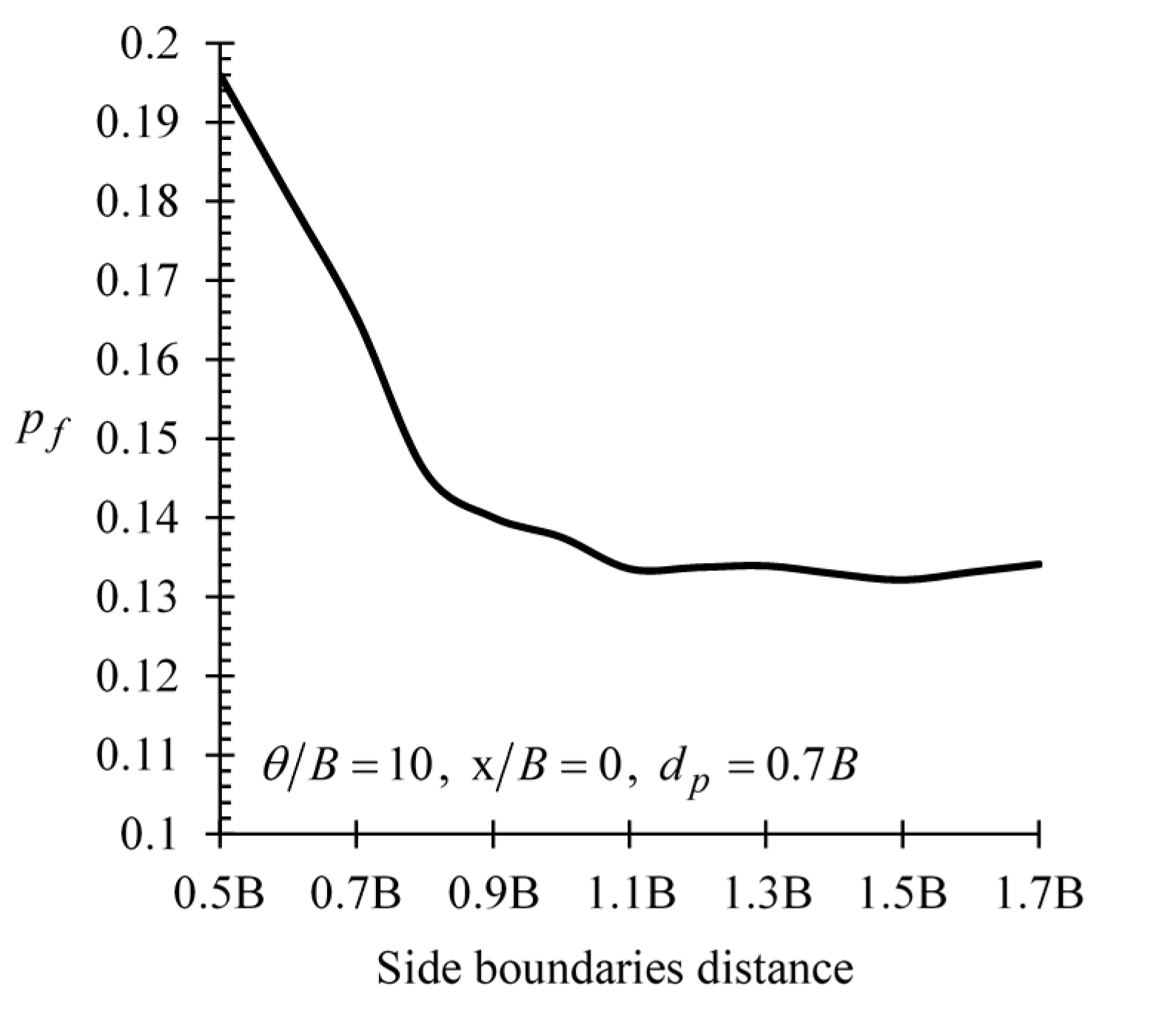
Appendix B. Stability of Numerical Results (Distance of Lateral Boundaries and Number of Realizations Considered in the RFEM Models)

In addition, Figure A1 shows the variation of p f with the number of realizations for various cases examined in this study. As it is inferred, the 10,000 realizations considered in the present analysis can be deemed sufficient. The p f vs. number of realizations curves of the figure in question refer to d p / B = 0.7 and x / B = 0, however, the same outcome is obtained for any sampling location.
The effect of the distance between the footing and the lateral boundaries in the finite element analysis carried out in the RFEM framework is shown in Figure A2. From this figure, it is inferred that a distance of 1.1B can be considered adequate in order to obtain reliable results. In this respect, the authors considered a distance equal to 1.7B.
Figure A1. p f vs. number of realizations by considering different (a) scaled scale of fluctuation values, (b) scaled horizontal sampling location values, (c) footing widths and (d) coefficient of variation of E; charts referring to d p / B = 0.7 B and x / B = 0.
Geosciences 10 00020 g0a1
Figure A2. p f vs. side boundaries distance from the edge of footing of width B = 1 m.
Geosciences 10 00020 g0a2

References

  1. Phoon, K.-K.; Kulhawy, F.H.; Grigoriu, M.D. Reliability-based design for transmission line structure foundations. Comput. Geotech. 2000, 26, 169–185. [Google Scholar] [CrossRef]
  2. Duzgun, H.S.B.; Yucemen, M.S.; Karpuz, C. A probabilistic model for the assessment of uncertainties in the shear strength of rock discontinuities. Int. J. Rock Mech. Min. Sci. 2002, 39, 743–754. [Google Scholar] [CrossRef]
  3. Tang, W.H.; Zhang, L. Quality assurance and risk reduction in foundation engineering. In Frontier Technologies Infrastructures Engineering: Structures and Infrastructures Book Series; Chen, S.-S., Ang, H.-S.A., Eds.; CRC Press: Florida, FL, USA, 2009; pp. 123–142. [Google Scholar]
  4. Jaksa, M.B.; Goldsworthy, J.S.; Fenton, G.A.; Kaggwa, W.S.; Griffiths, D.V.; Kuo, Y.L.; Poulos, H.G. Towards reliable and effective site investigations. Géotechnique 2005, 55, 109–121. [Google Scholar] [CrossRef]
  5. Griffiths, D.V.; Fenton, G.A.; Ziemann, H.R. Reliability of passive earth pressure. Georisk 2008, 2, 113–121. [Google Scholar] [CrossRef]
  6. Yang, R.; Huang, J.; Griffiths, D.V.; Sheng, D. Probabilistic stability analysis of slopes by conditional random fields. Geo-Risk 2017, 2017, 450–459. [Google Scholar]
  7. Ching, J.; Phoon, K.-K. Characterizing uncertain site-specific trend function by sparse Bayesian learning. J. Eng. Mech. 2017, 143, 4017028. [Google Scholar] [CrossRef]
  8. Yang, R.; Huang, J.; Griffiths, D.V.; Li, J.; Sheng, D. Importance of soil property sampling location in slope stability assessment. Can. Geotech. J. 2019, 56, 335–346. [Google Scholar] [CrossRef]
  9. Fenton, G.A.; Naghibi, F.; Hicks, M.A. Effect of sampling plan and trend removal on residual uncertainty. Georisk Assess. Manag. Risk Eng. Syst. Geohazards 2018, 12, 253–264. [Google Scholar] [CrossRef]
  10. Li, Y.J.J.; Hicks, M.A.A.; Vardon, P.J.J. Uncertainty reduction and sampling efficiency in slope designs using 3D conditional random fields. Comput. Geotech. 2016, 79, 159–172. [Google Scholar] [CrossRef] [Green Version]
  11. Yang, R.; Huang, J.; Griffiths, D.V.; Meng, J.; Fenton, G.A. Optimal geotechnical site investigations for slope design. Comput. Geotech. 2019, 114, 103–111. [Google Scholar] [CrossRef]
  12. Christodoulou, P.; Pantelidis, L.; Gravanis, E. The effect of targeted field investigation on the reliability of earth-retaining structures in active state. Appl. Sci. 2019, 9, 4953. [Google Scholar] [CrossRef] [Green Version]
  13. EN 1997-2. Eurocode 7-Geotechnical design-Part 2: Ground investigation and testing; CEN (European Committee for Standardization): Brussels, Belgium, 2007. [Google Scholar]
  14. AASHTO. AASHTO Lrfd Bridge Design Specifications; American Association of State Highway and Transportation Officials: Washington, DC, USA, 2010; ISBN 9781560514510. [Google Scholar]
  15. Fenton, G.; Griffiths, D.V. Risk Assessment in Geotechnical Engineering; Wiley: Hoboken, NJ, USA, 2008; ISBN 9780470178201. [Google Scholar]
  16. Orr, T.L.L. Managing Risk and Achieving Reliable Geotechnical Designs Using Eurocode 7. In Risk and Reliability in Geotechnical Engineering; Phoon, K.K., Ching, J., Eds.; CRC Press: Boca Raton, FL, USA, 2014; pp. 395–433. [Google Scholar]
  17. Ching, J.; Phoon, K.-K. Constructing multivariate distributions for soil parameters. Risk Reliab. Geotech. Eng. 2015, 1, 3–76. [Google Scholar]
  18. Huang, X.C.; Zhou, X.P.; Ma, W.; Niu, Y.W.; Wang, Y.T. Two-dimensional stability assessment of rock slopes based on random field. Int. J. Geomech. 2016, 17, 4016155. [Google Scholar] [CrossRef]
  19. Imanzadeh, S.; Denis, A.; Marache, A. Settlement uncertainty analysis for continuous spread footing on elastic soil. Geotech. Geol. Eng. 2015, 33, 105–122. [Google Scholar] [CrossRef]
  20. Rocscience Inc. RS2 Version 9.0-Finite Element Analysis for Excavations and Slopes 2019. Available online: https://www.rocscience.com/software/rs2 (accessed on 13 August 2018).
  21. Fenton, G.A.; Vanmarcke, E.H. Simulation of random fields via local average subdivision. J. Eng. Mech. 1990, 116, 1733–1749. [Google Scholar] [CrossRef] [Green Version]
  22. Vanmarcke, E.H. Probabilistic modeling of soil profiles. J. Geotech. Eng. Div. 1977, 103, 1227–1246. [Google Scholar]
  23. Paice, G.M.; Griffiths, D.V.; Fenton, G.A. Finite element modeling of settlements on spatially random soil. J. Geotech. Eng. 1996, 122, 777–779. [Google Scholar] [CrossRef]
  24. Fenton, G.A.; Griffiths, D.V. Probabilistic foundation settlement on spatially random soil. J. Geotech. Geoenviron. Eng. 2002, 128, 381–390. [Google Scholar] [CrossRef] [Green Version]
  25. Fenton, G.; Griffiths, D.V. Bearing-capacity prediction of spatially random c-ϕ soils. Can. Geotech. J. 2003, 40, 54–65. [Google Scholar] [CrossRef]
  26. Griffiths, D.V.; Huang, J.; Fenton, G.A. Influence of spatial variability on slope reliability using 2-D random fields. J. Geotech. Geoenviron. Eng. 2009, 135, 1367–1378. [Google Scholar] [CrossRef] [Green Version]
  27. Vanmarcke, E.H. Reliability of earth slopes. J. Geotech. Eng. Div. 1977, 103, 1247–1265. [Google Scholar]
  28. Soulie, M.; Montes, P.; Silvestri, V. Modelling spatial variability of soil parameters. Can. Geotech. J. 1990, 27, 617–630. [Google Scholar] [CrossRef]
  29. Cherubini, C. Data and Considerations on the Variability of Geotechnical properties of Soils. In Proceedings of the International Conference on Safety and Reliability, ESREL, Hannover, Germany, 22–26 September 1997; pp. 1583–1591. [Google Scholar]
  30. Popescu, R.; Prévost, J.H.; Deodatis, G. Effects of spatial variability on soil liquefaction: Some design recommendations. Geotechnique 1997, 47, 1019–1036. [Google Scholar] [CrossRef]
  31. Phoon, K.; Kulhawy, F. Characterization of geotechnical variability. Can. Geotech. J. 1999, 36, 612–624. [Google Scholar] [CrossRef]
  32. Schmertmann, J.H. Static cone to compute static settlement over sand. J. Soil Mech. Found. Div. 1970, 96, 1011–1043. [Google Scholar]
  33. Schmertmann, J.H.; Hartman, J.P.; Brown, P.R. Improved strain influence factor diagrams. J. Geotech. Geoenviron. Eng. 1978, 104, 1131–1135. [Google Scholar]
  34. Bergdahl, U.; Malmborg, B.S.; Ottosson, E. Plattgrundläggning; Svensk Byggtjänst: Stockholm, Sweden, 1993; ISBN 9173326623. [Google Scholar]
  35. EN 1997-1. Eurocode 7 Geotechnical Design—Part 1: General Rules; CEN (European Committee for Standardization): Brussels, Belgium, 2004. [Google Scholar]
  36. Canadian Standards Association. Canadian Highway Bridge Design Code. CAN/CSA-S6-14; Canadian Standards Association: Mississauga, ON, Canada, 2014. [Google Scholar]
  37. Kok-Kwang, P.; Kulhawy, F.H.; Grigoriu, M.D. Development of a reliability-based design framework for transmission line structure foundations. J. Geotech. Geoenviron. Eng. 2003, 129, 798–806. [Google Scholar]
  38. Fenton, G.A.; Naghibi, F.; Dundas, D.; Bathurst, R.J.; Griffiths, D.V. Reliability-based geotechnical design in 2014 canadian highway bridge design code. Can. Geotech. J. 2015, 53, 236–251. [Google Scholar] [CrossRef]
  39. JGS. Principles for Foundation Design Grounded on a Performance-Based Design Concept (GeoGuide); Japanese Geotechnical Society: Tokyo, Japan, 2004. [Google Scholar]
  40. Orr, T.L.L. Defining and selecting characteristic values of geotechnical parameters for designs to Eurocode 7. Georisk Assess. Manag. Risk Eng. Syst. Geohazards 2016, 11, 103–115. [Google Scholar] [CrossRef]
  41. White, J.; Yeats, A.; Skipworth, G. Tables for Statisticians, 3rd ed.; Nelson Thornes: Cheltenham, UK, 1979; ISBN 085950462X. [Google Scholar]
Figure 1. Typical random finite element mesh considering θ/B = 10. Figure showing the 20-element footing on the surface of a 88 × 40 (H × V) mesh.
Geosciences 10 00020 g001
Figure 2. Graphical representation of single sampling point ( d p ; Scenario A and B) and sampling domain length ( d d ; Scenario C and D) sampling strategies.
Geosciences 10 00020 g002
Figure 3. p f vs. d p / B example curves for various θ / B and x / B values: (a) θ / B = 0.5, (b) θ / B = 2, (c) θ / B = 5, (d) θ / B = 10, (e) θ / B = 20 and (f) θ / B = 50. The thick continuous line in (c) is for the anisotropic case and refers to the x / B = 0 case.
Geosciences 10 00020 g003
Figure 4. p f vs. d p / B example curves for θ = 10 m, x/B = 0 and different footing widths B.
Geosciences 10 00020 g004
Figure 5. p f vs. d p / B example relationships for θ/B = 10, x/B = 0 and different values of COV of E .
Geosciences 10 00020 g005
Figure 6. p f vs. d p / B example curves for different v values, x/B = 0 and θ / B = 10 .
Geosciences 10 00020 g006
Figure 7. vs. d d / B example curves for various θ / B and x / B values: (a) θ / B = 0.5, (b) θ / B = 2, (c) θ / B = 5, (d) θ / B = 10, (e) θ / B = 20 and (f) θ / B = 50. The thick continuous line in (c) is for the anisotropic case and refers to the x / B = 0 case.
Geosciences 10 00020 g007
Figure 8. vs. d d / B example curves for θ = 10 m, x/B = 0 and different footing widths B.
Geosciences 10 00020 g008
Figure 9. vs. d d / B example relationships for θ/B = 10, x/B = 0 and different COV values of E .
Geosciences 10 00020 g009
Figure 10. p f vs. d d / B example curves for θ/B = 10, x/B = 0 and different v values.
Geosciences 10 00020 g010
Figure 11. Graphical representation of the random field of E of Example #2 ( θ / B = 0.5; see Table 1).
Geosciences 10 00020 g011
Figure 12. Graphical representation of the random field of E of Example #3 ( θ / B = 5; see Table 1).
Geosciences 10 00020 g012
Figure 13. Graphical representation of the random field of E of Example #4 ( θ / B = 50; see Table 1).
Geosciences 10 00020 g013
Figure 14. ρ p r e d i c t e d / ρ a c t u a l vs. x/B curves for various dd/B values for Example #1 (a), #2 (b), #3 (c) and #4 (d). The random elastic modulus fields of Examples #1, #2, #3 and #4 are presented graphically in Figure 1, Figure 11, Figure 12 and Figure 13 respectively; see also Table 1.
Geosciences 10 00020 g014
Figure 15. ρ predicted / ρ actual vs. x / B curves using both mean and characteristic values (solid and dashed lines respectively). Figure referring to two sampling domain cases: (a) dd/B = 2 and (b) dd/B = 0.5.
Geosciences 10 00020 g015
Table 1. Summary of the characteristics of the soils used in the four examples (footing width B = 1 m).
ExampleRandom Field (s)Distribution μ E   ( Pa ) νCOV θ / B Figure (1)
#1ELog-normal10.250.3101
#2ELog-normal10.250.30.511
#3ELog-normal10.250.3512
#4ELog-normal10.250.35013
(1) Figures shown the random fields of E.

