A Generic Shear Wave Velocity Profiling Model for Use in Ground Motion Simulation

1
School of Civil Engineering, Guangzhou University, 230 Outer Ring Road, Guangzhou Panyu University City, Guangzhou 511400, China
2
Department of Infrastructure Engineering, The University of Melbourne, Grattan Street, Parkville, VIC 3010, Australia
*
Author to whom correspondence should be addressed.
Geosciences 2020, 10(10), 408; https://doi.org/10.3390/geosciences10100408
Submission received: 27 August 2020
/
Revised: 4 October 2020
/
Accepted: 10 October 2020
/
Published: 12 October 2020
Abstract
:This study presents a generic model for constructing shear-wave velocity (VS) profiles for various conditions that can be used for modeling the upper-crustal modification effects in ground motion simulations for seismic hazard analysis. The piecewise P-wave velocity (VP) profiling model is adopted in the first place, and the VS profile model is obtained by combining the VP profiling model and VS/VP model. The used VS/VP model is constructed from various field measurements, experimental data, or CRUST1.0 data collected worldwide. By making the best use of the regionally/locally geological information, including the thickness of sedimentary and crystalline layers and reference VS values at specific depths, the VS profile can be constructed, and thus the amplification behavior of VS for a given earthquake scenario can be predicted. The generic model has been validated by four case studies of different target regions world around. The constructed profiles are found to be in fair agreement with field recordings. The frequency-dependent upper-crustal amplification factors are provided for use in stochastic ground motion simulations for each respective region. The proposed VS profiling model is proposed for region-specific use and can thus make the ground motion predictions to be partially non-ergodic.
1. Introduction
Seismic hazard analysis for the regions of low-to-moderate seismicity can be very challenging for the acute scarcity of strong-motion data in these regions, and such regions include southeastern Australia (SEA) continent, eastern North America (ENA), and southeastern China (SEC). A realistic modeling approach for seismic hazard analysis purpose in stable continental regions (SCRs) and other intraplate regions (which are typically considered as low-to-moderate seismicity regions) can be achieved by combining the earthquake source effects, path effects, upper-crustal modification effects, and site conditions through stochastic simulations [1,2,3,4].
The regional path factor (which means path effect model) and local upper-crustal factor (which means the upper-crustal modification effect model and it is different from the widely used site factor, site-transfer function, site effect model, etc.) are of fundamental significance for modeling the ground motions in low-to-moderate seismicity regions with possibly low uncertainties and variabilities [5,6]. In practice, the regional path factor can be identical within a tectonic region in ground motion modeling, and such path factor can be representative of the characteristics of ground motion attenuations within the whole region (with the assumption that the path factor is ergodic within the region). A piece of good evidence for this statement is that most existing ground motion prediction equations (GMPEs) (except for non-ergodic GMPEs developed in some data-abundant regions. The sources factors and path factors are modeled to be site-specific in non-ergodic GMPEs [7]) can obtain a good match with the regional recording data by using one particular path (attenuation) factor, which is developed based on general broad geographical sub-division of a region, such as, Middle East [8], eastern North America [5,9,10,11,12], southeastern Australia [13,14]. The upper-crustal factor in the GMPEs mentioned above is defined in a broad geographical region as well (as the “reference rock site”), which indicates that the upper-crust conditions within the region are all identical. For example, people are using NEHRP (National Earthquake Hazard Reduction Program) B/C site (VS30 = 0.76 km/s, where VS30 is the time-averaged shear-wave velocity on the top 30 m of top sedimentary materials) [15] as the reference rock site to represent the upper-crustal condition for whole western North America (WNA) [16]. When these regional GMPEs are taken as the input for probabilistic seismic hazard analysis (PSHA) [17] for a specific region, similar results can be obtained for the same earthquake scenarios, tectonic classifications, and return periods. However, in real situations, the seismic loading requirements may differ dramatically for different locations within the region [18].
More explicitly speaking, the reason is that the upper-crustal factor within a tectonic region can change dramatically for different locations, especially for the regions with various geological conditions. For example, various geological upper-crustal conditions have been reported within the SEC region by [19]. The upper-crustal conditions within SEC are not identical, and the shear-wave velocity (SWV or VS) profiles for the three studied sub-regions (“SKP region”, “YZP region”, and “SCF region”) are very different. The enlisted GMPEs above would not provide relatively accurate estimates of ground motions that take the local variability (intra-regional uncertainty) into consideration within a region. Thus, a more comprehensive modeling methodology is required to cope with the local geological conditions of the local upper-crust to minimize the inter-regional and intra-regional uncertainty (which means to identify the upper-crustal factor from “ergodic” to partially “non-ergodic”).
Shear-wave velocity profiles are required to model the upper-crustal modification effects. Boore and Joyner [2] (abbreviated as BJ97 model in the following context) constructed a generic profiling model for seismic shear-wave velocity as a function of depth for generic rock (GR) site and generic very hard rock (GHR) site, based on borehole data and studies of upper-crustal velocities. Besides, Boore [16] (abbreviated as B16 model) put forward a simplified slowness (reciprocal of VS) interpolation method to construct the VS profile for a given VS30 value using the profiles of GR site (VS30 = 0.62 km/s) and GHR site (VS30 = 2.8 km/s). The VS profiles constructed by BJ model (which is abbreviated of BJ97 model and B16 model) are often used as the reference rock sites for a target region. The general process of constructing the VS profile for a specific VS30 value using BJ model is summarized in Boore and Joyner [2] and Boore [16]. The advantage of BJ model for constructing VS profiles is that it is quite simple and straightforward, which means it is convenient for practical engineering use, especially for the regions lacking abundant field measurements. However, this method is only proposed for broad application and not for any specific upper-crustal condition, which means that the VS profiles obtained by BJ model would contain large uncertainties when it is applied to some target regions.
To construct more reliable site-specific (local rather than regional) VS profiles, Chandler et al. [3] (abbreviated as CLT05 model in the following context) proposed a geology-based VS profile modeling approach based on modeling VP profile and VS/VP ratio. The global crust model CRUST2.0 (which can be found at https://igppweb.ucsd.edu/~gabi/crust2.html, last accessed in November 2019) is adopted to gather the geological information for target regions to construct and validate the proposed VS profile model. CLT05 model has been proved to be capable of constructing the VS profile for various upper-crustal conditions with a reasonable accuracy level. However, after a careful investigation by the authors, the VS/VP ratio modeled by the CLT05 model is not comparable to other studies (e.g., [20]), especially for the depth shallower than 4 km. Moreover, the CRUST2.0 (with a 2° × 2° resolution) database (which was used to obtain the geological information for constructing CLT05 model) has been superseded by researchers since 2013 as a more accurate CRUST1.0 (with a 1° × 1° resolution) database (which can be found at https://igppweb.ucsd.edu/~gabi/crust1.html, last accessed in November 2019) has been adopted nowadays. For the two reasons mentioned above, there is a requirement to propose a more rigorous and comprehensive VS profiling model.
The CRUST1.0 database is a global crustal model database at 1° × 1° resolution, which is an update of CRUST5.1 and CRUST2.0. The new model database incorporates an updated version of the global sediment thickness. The principal crustal types of the new model database are adopted from CRUST5.1, and the additional crustal types mark specific tectonic settings, such as continental rifts, continental shelves, and oceanic plateaus. In contrast to older models, the function of crustal types in the new model is limited to assigning elastic parameters to layers in the crystalline crust. CRUST1.0 consists of less than 40 crustal types, each of the 1° × 1° cells has a unique 8-layer crustal profile where the layers are: (1) water; (2) ice; (3) upper sediments; (4) middle sediments; (5) lower sediments; (6) crystalline upper crust; (7) crystalline middle crust; (8) crystalline lower crust. Parameters like compressional wave velocity (VP), shear wave velocity (VS), and crust density (ρ) are given explicitly for each layer (these parameters found the basis of this study). The updated correlation functions between Poisson’s ratio and VS, VP and VS, and VS, are all adopted from Brocher’s study which was published in 2005 [20], as this study used the comprehensive dataset to derive the correlation functions and is generally acknowledged by scholars worldwide. More introduction of global crustal models can be found from the paper published by Chandler et al. [3].
The purpose of this study is to propose a more valid and comprehensive VS profiling model, which can be used to construct the region-specific VS profiles for various upper-crustal conditions and can be incorporated into stochastic simulations of ground motions as well as seismic hazard assessment procedures. The model is based on the available geological information which can be obtained from the CRUST1.0 database as well as existing field recordings. The well-known piecewise P-wave model is briefly introduced in Section 2.1. A newly developed VS/VP model as a function of depth (Z) using data from various sources worldwide is put forward in Section 2.2, and 6 frequently encountered cases with the corresponding VS models are identified in Section 2.3. Four case studies from different tectonic regions are conducted in Section 3 to validate the proposed VS profiling model. The final frequency-dependent upper-crustal amplification factor for each region is provided, which can be used in stochastic simulation procedures directly.
2. Shear-Wave Velocity Modeling
This section introduces the detailed modeling process of the near-source shear-wave velocity (VS) profile within the upper-crust, which can be used for constructing the frequency-dependent upper-crustal amplification factor. As mentioned above, according to the conclusion obtained by Brocher [20], the estimates of compressional wave velocity (VP) are reasonably accurate in most cases. However, the estimates of shear-wave velocity (VS) are not accurate in most cases [21,22]. The reason is that the relationship between VP and VS are always inappropriate. Thus, in this study, VP profiling model would be adopted directly from previous studies in the first place. Then, VS/VP would be modeled using updated recording data collected from various sources. The final Vs profile would then be modeled by combining the VP profile model and VS/VP model.
2.1. Compressional Wave Velocity (VP) Profiling Model
The previous studies show that the compressional wave is closely related to crustal structure, depth, temperature, the geological age of rock formation, and even chemical compositions of the sediments [23,24,25,26]. For seismic hazard analysis purpose, the modern 3D VP profiles obtained from seismic refraction and reflection surveys are not convenient for use in stochastic ground motion procedures, as the purpose of most seismic velocity measurements is for determining site-specific properties, not for developing any specific mathematic expressions [27,28,29]. In this study, all seismic wave profiles will be modeled as the functions of depth for convenient engineering use in stochastic ground motion simulation procedures, which is suggested by other related studies [2,16]. The functional form developed by Chandler et al. [3] is adopted. The piecewise functional form of the VP model is summarized as Equation (1):
where Z is the depth in the unit of km; VP0.03, VPZS, VPZC, VP8 are the reference VP values at the depth of 0.03 km, ZS km, ZC km, and 8 km, respectively; and ZS, ZC are the thickness of the upper sedimentary crustal layer and the total sedimentary crustal layers with the unit of km [3]. The whole function can be illustrated by Figure 1.
The validation of this VP model can be found in Chandler et al. [3], and the results showed that the VP model is valid in most cases. Therefore, this VP model is adopted directly.
2.2. Modeling of VS/VP
The VS–VP relationship is essential for various engineering applications, including the analysis of reservoir geomechanical properties for studying seismic ground motions. However, VS records are often not available for target regions due to technological limitations. Alternatively, VS can be obtained from empirical prediction equations based on the records of VP. In the BJ97 [2] model, Boore and Joyner obtained the VS profiles generally from two generic approaches: one is the VS data from boreholes in the upper 4 km; another one is through the data of the VP profile and the VS–VP relationship (VS/VP = 1/) for the depth larger than 4 km. In this study, the VS profiles will be derived from VP completely for all depths (as a generic approach). Thus, the VS–VP relationship is of extreme importance to obtain a relatively accurate VS profile (assume VP profile is valid). Recording data from multiple sources around the world are gathered for modeling VS/VP. These data are selected randomly world around to make the VS/VP to be as “generic” as possible. Detailed information about data collected for modeling VS/VP is summarized in Table 1.
Thorough regression analysis for the ratio (VS/VP) is conducted using this dataset. As the data set is collected world around, large uncertainties should be prudently considered during the modeling process. Chandler et al. [3] provided a power functional format for the VS/VP ratio as it is convenient to combine it with the VP model. In this study, the authors will adopt the power functional format again but in a more rigorous way. The detailed modeling procedures are stated below.
Firstly, as Poisson’s ratio (denoted as “” in this study) is closely related to the VS/VP ratio, it is important to clarify it before the determination of the VS/VP ratio. For shallow depth, value depends largely on the depth and saturation of the medium. However, it is suggested by Boore and Joyner [2] that can be fixed at 0.25 for the depth larger than 4 km, as the lithostatic pressure at these depths (about 1 kbar) can make most cracks be closed. From the study of Brocher [20], the functional form is expressed in Equation (2), which is the same one shown in Chandler et al. [3], which is obtained from the elastic wave propagation theory in a homogeneous medium:
where is Poisson’s ratio.
For the depth larger than 4 km, VS/VP = 0.577 (being ), which is suggested by the BJ97 model and CLT05 model. According to this study, for the depths between 2 and 4 km, the VS/VP value also keeps constant (shown in Figure 2). To be more explicit, the authors found that below the depth of 2 km, VS/VP = 0.577 can obtain similar regression goodness (with no apparent change in mean residual, which is defined by Equation (3), for the depths larger than 2 km). Therefore, for the depth larger than 2 km, VS/VP is set to be a fixed value 0.577 in this study (Zone C in Figure 2):
where is the mean residual of all depth (the upper-limit of depth is 50 km if no specific note is given); N is the total number of recording data collected from various sources, which equals to 193 in this study; is the field recorded VS/VP value; is the predicted VS/VP value, which is obtained from the proposed model in this study.
Secondly, for the depth smaller than 2 km, the general regression technique is performed. Single-segment line (log(VS/VP) vs. log(Z)) is adopted in the first time, the mean residual value (0.21) indicates the regression can be improved to some extent. In this case, two segments are considered. Different transition depth values (0.1, 0.2, 0.4, and 1 km) are evaluated. The first segment would only consider modeling the dataset with the depth smaller than the transition depth. The authors found that the mean residual can achieve the lowest value for the data with depth less than 0.2 km. Thus, the transition depth is set to be 0.2 km in this study (shown as Zone A in Figure 2).
Lastly, another segment (from 0.2 to 2.0 km) is modeled to connect the two segments modeled in the previous steps, and the result is shown as Zone B in Figure 2.
As shown in Figure 2, the proposed tri-linear VS/VP model can represent the collected data (listed in Table 1) with a reasonable level of accuracy (with the mean residual of 0.089). The point should be noted is that this generic VS/VP model is proposed (as a sole function of depth) for convenient use in engineering seismology and other related studies, other parameters like material type, temperature, and pressure are not considered.
The overall VS/VP model is expressed in Equation (4):
0.5684(Z/0.2)0.163 Z ≤ 0.2,
0.577(Z/2)0.00652 0.2 < Z ≤ 2.0,
0.577 Z > 2.0.
0.577(Z/2)0.00652 0.2 < Z ≤ 2.0,
0.577 Z > 2.0.
To evaluate the rationality of the proposed VS/VP model in this study, four existing VS–VP relationship equations obtained from various data recordings globally are adopted in this study for comparison purpose (the equations can be found in Table 2). Note that all the selected equations, Cea85 [42], Han86 [43], B05 [20], CLT05 [3] are used as generic models for global conditions. To illustrate the VS/VP ratio with the change of depth, the generic VS profile of NEHRP (National Earthquake Hazard Reduction Program) B/C site (VS30 = 0.76 km/s) is adopted and VS/VP is computed based on this profile. The comparison details are shown in Figure 3 for depth ranging from 0.001 to 100 km for all models.
As shown in Figure 3, except for the CLT05 model, other models can obtain similar estimates of VS/VP for different depths. It can be seen that the proposed VS/VP by this study matches well with the B05 model, which was developed from comprehensive datasets [20] and widely acknowledged globally. The CLT05 model gives smaller estimates of VS/VP at the depth 0.01 to 4 km, compared with other models. The Cea85 model gives similar estimates of VS/VP at the depth smaller than 2.0 km, compared with the B05 model and the proposed model in this study. The Han86 model gives a similar estimate of VS/VP at the depth of 0.2 km, and larger estimates of VS/VP at other depths, compared with the B05 model and the proposed model in this study. The mean residuals (using Equation (3)) between the proposed model and Cea85, Han86, B05, and CLT05 models are 0.039, 0.047, 0.012, 0.053 respectively, which indicates that the proposed VS/VP model is close to the value given by the B05 model for all depths.
2.3. Shear-Wave Velocity Profile Modeling
Based on the results obtained from Section 2.1 and Section 2.2, the VS profile can be modeled by combining the VP profile and VS/VP model. The detailed modeling processes are stated below.
For the Zone I and Zone A (Zone IA):
For the Zone I and Zone B (Zone IB):
For the Zone I and Zone C (Zone IC):
Similarly, the VS model for the Zone IIIA, IIIB, and IIIC are expressed as Equations (8)–(10), respectively:
VS = VS0.2 (Z/0.2)0.2463,
VS = VS2 (Z/2)0.0899,
VS = VS8 (Z/8)0.0833.
For the transition zone (II):
in which:
VS = VSZC (Z/ZC)n,
According to the relative positions of ZS and ZC to the identified marker depth 0.2 and 2.0 km, there would be 6 (which is 3!) different cases, which are illustrated in Figure 4.
The detailed functional expressions for the 6 identified cases and their corresponding zones are summarized in Table 3.
In all cases, Zone II is a transition zone that is used to connect the upper zone and the lower zone. Thus, the functional form is the same, except for the value of exponent “n”. In all cases, n is expressed by Equation (12). As the values of VSZC and VSZS are changing for different cases, the value of n will be differing accordingly case by case.
The estimation of ZC and ZS values are essential for constructing reasonable local VS profiles. The detailed three approaches for estimating ZC and ZS values are given below.
(i) If sufficient and reliable field measurements of the crustal VS profile are available, the values of ZS and ZC can be adjusted to achieve a good match with the local field measurements;
(ii) If no field measurements can be obtained to determine ZS and ZC, then ZS and ZC can be taken as the averaged thickness of the upper sediment layer and averaged total sediment layers (provided by CRUST1.0), respectively.
To make the overall process of VS profile construction more convenient for use, a MATLAB-based computer program is provided alongside this article. The flowchart of the program is shown in Figure 5, and the program can be downloaded from the link: https://github.com/Y-Tang99/GMSS.
3. Validation of the Proposed VS Profiling Model
In this section, the VS profiling model proposed in Section 2 will be applied to four different tectonic regions. Local VS profiles obtained from technical measurements at each region will be used for comparison and validation purpose. The selected regions are the Melbourne Region (located in southeastern Australia), St. Louis Metro Region (located in central eastern North America), Hong Kong Region (located in southeastern China), and northern Switzerland (located in central western Europe). These regions are selected from typical intraplate regions with low-to-moderate seismicity. The detailed location information of sampling points used for collecting geological information from CRUST1.0 is listed in Table 4 and shown in Figure 6. These sampling points are selected because the local field measurements of VS profiles are collected from these points. The parameters used for constructing VS profiles are summarized in Table 5.
Melbourne Region locates at Victoria state in southeastern Australia. The field measurements of the 5 selected sites in different suburbs around Melbourne metropolitan area are obtained from the passive seismic investigation technique called the spatial auto-correlation (SPAC) method [44]. A series of surveys were carried out to get the VS profiles down to the depth of around 0.1 km into Silurian mudstone. The St. Louis Metro Region is located at Missouri urban area in central eastern North America (CENA). The filed VS profiles of the 6 sites are determined from the surface wave measurements using the multi-channel analysis of surface waves (MASW) geological technique to the depth of around 0.03 km of upper sedimentary bedrock or surficial material [45]. Hong Kong Region locates at southeastern China. The field VS recordings are obtained from several sources: for the depth up to around 0.1 km, the VS data are collected from extensive borehole data; for the depth up to 1.5 km, the VS data are obtained from the SPAC method and short-period group velocity (T = 0.4–1.3 s) dispersion of Rg waves generated by quarry blasts [46]. Northern Switzerland is in central western Europe. The field VS profiles are obtained from array processing of ambient noises [47] as well as from interpretation of seismic refraction and reflection studies [48,49] for the depth up to around 3.0 km. For all selected regions, the VS data for the depth exceeding 4 km are obtained from the web-based global crust model CRUST1.0 [50]. The average field measurement for each region is obtained from the mean value of the field measurements at each depth.
For each selected region, the CLT05 model and BJ model will be adopted for comparison purposes. The overall results are shown in Figure 7, and the residuals (defined as the difference between average field measurements and the model predictions) are shown in Figure 8 for each region.
To use the generic VS profiling model proposed by this study, the ZS and ZC are required to be determined in the first place. The followed step is to determine which case model (listed in Table 3) is suitable for use in the target region. The next step is to determine the reference VS values at certain depths and the exponential value (n). The final step is to construct the VS profile for the target region. To make it clearer, Melbourne Region is taken as an example:
Step (i): ZS and ZC values are determined from the average value of the 5 sampling points (for each sampling point, the detailed ZS and ZC value can be collected from CRUST1.0 database). In this study, ZS = 0.05 km and ZC = 4.0 km;
Step (ii): Because ZS < 0.2 < 2 ≤ ZC, the Case 4 VS profiling model should be used in this study (listed in Table 3);
Step (iii): Ideally, the reference VS values should be determined from local field measurements, while the VS values collected from CRUST1.0 database can be used if valid field measurements are not available. For the Case 4 profiling model, four reference VS values need to be determined: VSZS, VSZC, VSZI, and VS8. VSZS = 1.33 km/s and VSZI = 1.1 km/s (in this case VSZI = VS0.03), and they are determined from average field measurement. VSZC = 3.3 km/s and VS8 = 3.5 km/s, which are determined from the CRUST1.0 database. “n” is finally determined using Equation (12), which is 0.21 in this study.
Step (iv): Construct VS profile for all depths and eliminate any possible abnormal points by a double check procedure. The final VS profile constructed for the Melbourne Region is shown as the red line in Figure 7a.
Figure 7a indicates that all model estimates can get the alignment with the field measurements with a reasonable level of accuracy. The average residual of for the three models (this study, CLT05 model and BJ model) is 0.103, 0.107, and 0.075 respectively, which is shown in Figure 8a.
For the St. Louis Metro Region, the situation is slightly different from other selected regions as this region is located at St. Louis Metropolitan area and the sampling sites are quite close to each other. This site is characterized as the NEHRP rock site (0.62 km/s < VS30 < 1.5 km/s), which is the same as the Melbourne Region and northern Switzerland, while Hong Kong Region is a typical hard rock site (VS30 > 1.5 km/s) [15]. Repeating Step (i) to Step (iv), and the Case 2 profiling model is suitable for this regionFigure 7b and Figure 8b indicate the model proposed by this study performs slightly better than another two models (CLT05 model and BJ model).
For the Hong Kong Region, the average depth of the sedimentary layer indicates that CRUST1.0 is very small. Considering the quite small VS gradient at shallow depths indicated by the field measurements, the exponential value (which indicates the gradient of VS) in the VS profiling model needs to be small accordingly. However, the exponential value for shallow depths (<0.2 km) is fixed at 0.3297 in all case models listed in Table 5, which is too large to represent the actual VS gradient. Based on these considerations, the ZS value is adjusted to be 0.001 km to make the shallow depth zone located in Zone II (shown in Figure 4). In this case, a variable exponential value (“n”) can be obtained and can thus be adjusted to mimic the VS gradient of VS obtained from field measurements. As ZC is determined as 1.0 km from CRUST1.0 database, the Case 5 profiling model should be adopted in this region (ZS < 0.2 < ZC ≤ 2). The results are shown in Figure 7c and Figure 8c, and they indicate that the model proposed by this study performs better than CLT05 model and BJ model, especially at shallow depths (<0.01 m).
Similar to Hong Kong Region, the sedimentary layer depth of northern Switzerland is very small indicated by CRUST1.0, and the field VS gradient is small at shallow depths. The value of ZS is set to be 0.001 km, and the Case 5 profiling model is adopted. Final VS profiles and the corresponding residuals are shown in Figure 7d and Figure 8d, respectively. The results also indicate the model proposed by this study performs better than the CLT05 model and BJ model for this region.
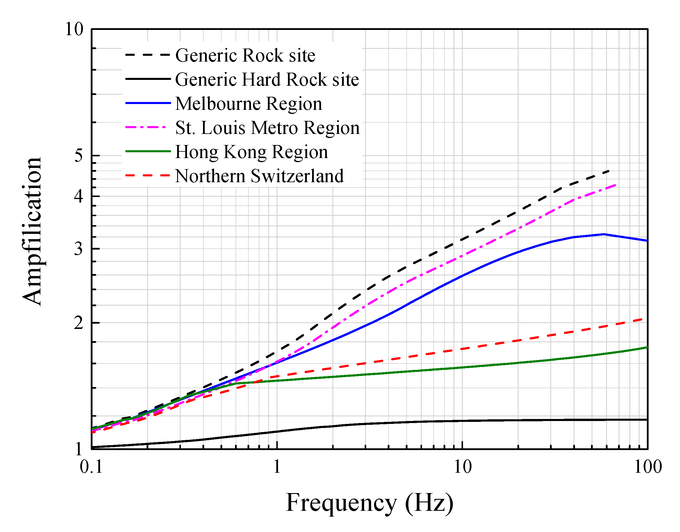
The upper-crust amplification can be obtained from the VS profile and density profile. The amplification factor obtained from the quarter wavelength approximation (QWA) method for each region is provided in this study. The frequency-dependent amplification is computed using Equation (13):
where and are the density and VS near the seismic source; and are the time-weighted average density and VS within the crust. In this study, the units of and are g/cm3 and km/s, respectively. The density profiles () for each region are determined using the equations provided in [15]. More detailed information about the QWA method can be found in [2]. The amplification for each target region can be found in Figure 9.
4. Discussion
Rather than providing an approach of estimating the site indicator VS30, this study intends to provide an approach to obtain the shear-wave velocity profile for modeling the upper-crustal modification effects. There are generally three different methods to estimate the upper-crustal factor [51]. The most widely used method is the reference-rock-site method, which is based on the comparison of recorded motions on the local site to those at an identified reference rock site. The reference rock site is often set to be identical for the whole target region (e.g., WNA). The second method is “H/V” (the ratio of horizontal component motions to vertical component motions) method, which is based on the assumption that vertical component ground motions are not influenced by the local site conditions significantly. Thus, the H/V ratio can be a good indicator of local site condition influence on the horizontal component ground motions [52]. This method is similar with the receiver-function method initially used for studying the earth upper mantle and crust from teleseismic recordings [53], and many existing GMPEs derive the site factor using this method [5,10,13,54]. However, this method often does not consider the effect of upper-crust (the depth is too small). Moreover, a criticism of the “H/V” method summarized by Atkinson and Boore [5] is that the “H/V” estimate is largely a measure of Rayleigh wave ellipticity and the “H/V” ratio would be largely controlled by site response when it applied to body waves which are measured from earthquakes [52]. Many existing GMPEs are developed by combining the reference rock site method and “H/V” method [12,13]. The third method is the theoretical wave-propagation modeling of upper-crust modification effect (theoretically modeling method). In this method, two separate effects are considered to model the upper-crustal modification effects: upper-crustal amplification effect of the seismic waves when they cross the boundary between different mediums and the upper-crustal attenuation effect which is associated with the transmission quality of the upper-crustal layers (the attenuation effect is beyond the scope of this study). The two effects mentioned above have been observed from the instrumental records from deep drill-holes in active seismic areas [55]. Chen [51] proved that the third method could be comparable to “H/V” method for various upper-crustal conditions.
In the theoretically modeling method, VS and density (ρ) profiles are essentially required to model the upper-crustal amplification effect. The quarter wavelength approximation (QWA) and the square root impedance (SRI) method [2,56] are used to compute the frequency-dependent upper-crustal amplification factor. This method will be adopted in this study to compute the upper-crustal amplification factor.
Seismic wave velocity (including compressional velocity (VP) and shear-wave velocity (VS)) model can be obtained from non-invasive seismic techniques, including refraction and reflection surveys [57,58], and invasive seismic techniques, including borehole methods [59]. However, most of the seismic wave velocity structures (or profiles) directly obtained by these approaches are often used for deterministically analyzing seismic hazard purpose [60,61,62]. The so obtained seismic wave velocity structures are not convenient (and often not available in low-to-moderate seismicity regions) for use in stochastic ground motion simulations because no parameterized functional form is given. Therefore, seismic wave profile modeling still requires more attention for convenient engineering application, especially for the regions where stochastic simulations are required for seismic hazard analysis.
With the rapid development of the non-ergodic PSHA, the requirement of the site-specific GMPE modeling becomes more acute. This study mainly provides an approach to minimize the uncertainties of upper-crustal modification effects in the modeling procedures, which would help to reduce the aleatory uncertainty in PSHA and make the hazard curve more reliable. Figure 7, Figure 8 and Figure 9 indicate that, the shallower part of VS profiles critically influences the estimates of upper-crust modification effects as they contain large uncertainties, which means the ground motions at higher frequencies would be more impacted. In practical use, users should pay more attention to the shallower part of the constructed VS profile for the target region and make sure the uncertainties are fully considered in ground motion simulations, and in any following procedures such as PSHA or dynamic structural response analysis using the simulated accelerograms.
5. Conclusions
This study proposed a generic VS profiling model which can be used for stochastic simulation of ground motions and seismic hazard assessment purposes. The proposed model is mainly designed for rock site conditions and should be avoided for any arbitrary applications. A comprehensive VS/VP relationship, as a function of depth, has been proposed in the first step based on various field recording data collected worldwide. The region-specific VS profile could be constructed using the functional formats provided in Table 3 and the algorithm shown in Figure 5. The geological information needed for VS profile construction includes the thickness of the upper sedimentary layer and the total thickness of all sedimentary layers (collected from CRUST1.0 with the longitude and latitude of the sampling points in the target region); and the reference VS values at certain depths (collected from field recordings or CRUST1.0). The detailed steps of constructing VS profiles have been provided. The validation of the proposed model has been made by 4 case studies in different tectonic regions in the world.
Author Contributions
Conceptualization, Y.T.; methodology, Y.T.; software, Y.T.; validation, Y.T. and X.X.; formal analysis, Y.T. & J.S.; investigation, Y.T., X.X., & J.S.; resources, Y.T.; data curation, Y.T. & J.S.; writing—original draft preparation, Y.T.; writing—review and editing, X.X. & J.S.; visualization, Y.T.; supervision, Y.Z. & X.X.; project administration, Y.Z.; funding acquisition, X.X. & Y.Z. All authors have read and agreed to the published version of the manuscript.
Funding
The authors are funded by Research Startup Funding (Funding Project No.: 51778162, 2018/01–2021/12) at Guangzhou University.
Acknowledgments
The original idea of this work proposed by Dr. Hing-Ho Tsang at the Swinburne University of Technology and Prof. Nelson Lam at The University of Melbourne is sincerely acknowledged.
Conflicts of Interest
The authors declare no conflict of interest.
Data Availability
The data used in this study can be found at the Mendeley Data, and the link can be available upon requests.
References
- Boore, D.M. Simulation of Ground Motion Using the Stochastic Method. Pure Appl. Geophys. 2003, 160, 635–676. [Google Scholar] [CrossRef] [Green Version]
- Boore, D.M.; Joyner, W.B. Site Amplifications for Generic Rock Sites. Bull. Seismol. Soc. Am. 1997, 8787, 327–341. [Google Scholar]
- Chandler, A.M.; Lam, N.T.K.; Tsang, H.H. Shear wave velocity modelling in crustal rock for seismic hazard analysis. Soil Dyn. Earthq. Eng. 2005, 25, 167–185. [Google Scholar] [CrossRef]
- Lam, N.T.K.; Wilson, J.; Hutchinson, G. Generation of Synthetic Earthquake Accelerograms Using Seismological Modelling: A Review. J. Earthq. Eng. 2000, 4, 321–354. [Google Scholar] [CrossRef]
- Atkinson, G.M.; Boore, D.M. Earthquake Ground-Motion Prediction Equations for Eastern North America. Bull. Seismol. Soc. Am. 2006, 96, 2181–2205. [Google Scholar] [CrossRef]
- Lam, N.T.K.; Wilson, J.L.; Chandler, A.M.; Hutchinson, G.L. Response spectral relationships for rock sites derived from the component attenuation model. Earthq. Eng. Struct. Dyn. 2000, 29, 1457–1489. [Google Scholar] [CrossRef]
- Abrahamson, N.A.; Kuehn, N.M.; Walling, M.; Landwehr, M. Probabilistic Seismic Hazard Analysis in California Using Nonergodic Ground-Motion Models. Bull. Seismol. Soc. Am. 2019, 109, 1235–1249. [Google Scholar] [CrossRef]
- Ambraseys, N.N.; Douglas, J.; Sarma, S.K.; Smit, P.M. Equations for the estimation of strong ground motions from shallow crustal earthquakes using data from Europe and the Middle East: Horizontal peak ground acceleration and spectral acceleration. Bull. Earthq. Eng. 2005, 3, 1–53. [Google Scholar] [CrossRef] [Green Version]
- Atkinson, G.M.; Boore, D.M. Ground-Motion Relations for Eastern North America. Bull. Seismol. Soc. Am. 1995, 85, 17–30. [Google Scholar]
- Atkinson, G.M. Empirical Attenuation of Ground Motion Spectral Amplitudes in Southeastern Canada and the Northeastern United States. Bull. Seismol. Soc. Am. 2004, 94, 1079–1095. [Google Scholar] [CrossRef]
- Atkinson, G.M. Ground-Motion Prediction Equations for Eastern North America from a Referenced Empirical Approach: Implications for Epistemic Uncertainty. Bull. Seismol. Soc. Am. 2008, 98, 1304–1318. [Google Scholar] [CrossRef]
- Yenier, E.; Atkinson, G.M. Regionally Adjustable Generic Ground-Motion Prediction Equation Based on Equivalent Point-Source Simulations: Application to Central and Eastern North America. Bull. Seismol. Soc. Am. 2015, 105, 1989–2009. [Google Scholar] [CrossRef]
- Allen, T.I. Stochastic ground-motion prediction equations for southeastern australian earthquakes using updated source and attenuation parameters. Geosci. Aust. Rec. 2012, 69, 55. [Google Scholar]
- Somerville, P.; Graves, R.; Collins, N.; Song, S.G.; Ni, S.; Cummins, P. Source and ground motion models for australian earthquakes. In Proceedings of the Annual Conference of the Australian Earthquake Engineering Society (AEES), Newcastle, Australia, 11–13 December 2009. [Google Scholar]
- BSSC. 2000 Edition NEHRP Recommmded Provisions for Seismic Regulations for New Buildings and Other Structures. FEMA 2001, 368–369. [Google Scholar]
- Boore, D.M. Short Note: Determining Generic Velocity and Density Models for Crustal Amplification Calculations, with an Update of the Boore and Joyner (1997) Generic Amplification for Vs(Z) = 760 m/s. Bull. Seismol. Soc. Am. 2016, 106, 316–320. [Google Scholar] [CrossRef]
- Castaños, H.; Lomnitz, C. PSHA: Is it science? Eng. Geol. 2002, 66, 315–317. [Google Scholar] [CrossRef]
- Lam, N.T.K.; Tsang, H.H.; Lumantarna, E.; Wilson, J.L. Minimum loading requirements for areas of low seismicity. Earthq. Struct. 2016, 11, 539–561. [Google Scholar] [CrossRef]
- Tsang, H.H.; Sheikh, M.N.; Lam, N.T.K.; Chandler, A.M.; Lo, S.H. Regional differences in attenuation modelling for Eastern China. J. Asian Earth Sci. 2010, 39, 441–459. [Google Scholar] [CrossRef] [Green Version]
- Brocher, T.M. Empirical relations between elastic wavespeeds and density in the Earth’s crust. Bull. Seismol. Soc. Am. 2005, 95, 2081–2092. [Google Scholar] [CrossRef]
- Brocher, T.M.; Brabb, E.E.; Catchings, R.D.; Fuis, G.S.; Fumal, T.E.; Jachens, R.A. A crustalscale 3-D seismic velocity model for the San Francisco Bay area, California. Eos Trans. AGU 1997, 78, F435–F436. [Google Scholar]
- Fletcher, J.B.; Boatwright, J.; Lindh, A.G. Wave propagation and site response in the Santa Clara Valley. Bull. Seismol. Soc. Am. 2003, 93, 480–500. [Google Scholar] [CrossRef]
- Christensen, N.I. Seismic Velocity Structure and Composition of the Continental Crust: A Global View. J. Geophys. Res. 1995, 100, 9761–9788. [Google Scholar] [CrossRef]
- Downs, H. The Nature of the Lower Continental Crust of Europe: Petrologic and Geochemical Evidence from Xenoliths. Phys. Earth. Planet. Inter. 1993, 79, 195–218. [Google Scholar] [CrossRef]
- Faust, L.Y. Seismic Velocity as a Function of Depth and Geologic Time. Geophysics 1951, 16, 192–206. [Google Scholar] [CrossRef]
- Magistrale, H.; McLaughlin, K.; Day, S. A Geological-based 3D Velocity Model of the Los Angeles Basin Sediments. Bull. Seismol. Soc. Am. 1996, 86, 1161–1166. [Google Scholar]
- Fliedner, M.M.; Klemperer, S.; Christensen, N.I. Three-dimensional Seismic Model of the Sierra Nevada arc California and Its Implications for Crustal and Upper Mantle Composition. J. Geophys. Res. 2000, 105, 10899–10921. [Google Scholar] [CrossRef]
- Lee, R.L.; Bradley, B.A.; Ghisetti, F.C.; Pettinga, J.R.; Hughes, M.W.; Thompson, E.M. A geology-based 3D seismic velocity model of canterbury, New Zealand. In Proceedings of the 2015 New Zealand Society for Earthquake Engineering Annual Conference (NZSEE), Rotorua, New Zealand, 10–12 April 2015. [Google Scholar]
- Zhao, B.; Zhang, Z.; Bai, Z.; Badal, J.; Zhang, Z. Shear Velocity and Vp/Vs Ratio Structure of the Crust beneath the Southern Margin of South China Continent. J. Asian Earth Sci. 2013, 62, 167–179. [Google Scholar] [CrossRef]
- Kwong, J.S.M. Pilot Study on the Use of Suspension PS Logging; Technical Note TN 2/98; GEO. Hong Kong Government: Hong Kong, China, 1998.
- Tam, K.W. Anisotropy in Seismic Wave Velocity in Jointed Rocks in Hong Kong. Master’s Thesis, The University of Hong Kong, Hong Kong, China, 2002. [Google Scholar]
- Malin, P.E.; Gillespie, M.H.; Leary, P.C.; Henyey, T.L. Crustal structure near Palmdale, California, from borehole-determined ray parameters. Bull. Seismol. Soc. Am. 1981, 71, 1783–1804. [Google Scholar]
- Stewart, R.R.; Turpening, R.M.; Toksoz, M.N. Study of a subsurface fracture zone by vertical seismic profiling. Geophys. Res Lett. 1981, 8, 1132–1135. [Google Scholar] [CrossRef]
- Archuleta, R.J. Analysis of near source static and dynamic measurements from the 1979 Imperial Valley earthquake. Bull. Seismol. Soc. Am. 1982, 72, 1927–1956. [Google Scholar]
- Brocher, T.M.; Fuis, G.S.; Lutter, W.J.; Christensen, N.I.; Ratchkovski, N.A. Seismic Velocity Models for the Denali Fault Zone along the Richardson Highway, Alaska. Bull. Seismol. Soc. Am. 2004, 94, 85–106. [Google Scholar] [CrossRef] [Green Version]
- Boore, D.M. P- and S-Velocities from Surface-to-Borehole Logging (Open-File Report). (30–191). 2003. Available online: http://www.daveboore.com/data_online.html (accessed on 5 October 2019).
- Baise, L.G.; Dreger, D.S.; Glaser, S.D. The Effect of Shallow San Francisco Bay Sediments on Waveforms Recorded during the Mw 4.6 Bolinas, California. Bull. Seismol. Soc. Am. 2003, 93, 465–479. [Google Scholar] [CrossRef]
- Wang, Z.; Butler III, D.T.; Woolery, E.W.; Wang, L. Seismic Hazard Assessment for the Tianshui Urban Area, Gansu Province, China. Int. J. Geophys. 2012, 2012, 1–10. [Google Scholar] [CrossRef] [Green Version]
- Ramirez-Guzman, L.; Zeng, Y.; Mooney, W.D. Rupture History of the 2008 Mw 7.9 Wenchuan, China, Earthquake: Evaluation of Separate and Joint Inversions of Geodetic, Teleseismic, and Strong-Motion Data. Bull. Seism. Soc. Am. 2013, 103, 353–370. [Google Scholar]
- Lin, G.; Amelung, F.; Shearer, P.M.; Okubo, P.G. Location and size of the shallow magma reservoir beneath Kilauea caldera, constraints from near-source Vp/Vs ratios. Geophys. Res. Lett. 2015, 42, 8349–8357. [Google Scholar] [CrossRef] [Green Version]
- Bhowmick, S. Role of Vp/Vs and Poisson’s Ratio in the Assessment of Foundation(s) for Important Civil Structure(s). Geotech. Geol. Eng. 2017, 35, 527–534. [Google Scholar] [CrossRef]
- Castagna, J.P.; Batzle, M.L.; Eastwood, R.L. Relationships between compressional-wave and shear-wave velocities in clastic silicate rocks. Geophysics 1985, 50, 571–581. [Google Scholar] [CrossRef]
- Han, D.H. Effects of Porosity and Clay Content on Acoustic Properties of Sandstones and Unconsolidated Sediments. Ph.D. Thesis, Stanford University, Stanford, CA, USA, 1986. [Google Scholar]
- Roberts, J.; Asten, M.W.; Tsang, H.H.; Venkatesan, S.; Lam, N.T.K. Shear wave velocity profiling in melbourne silurian mudestone using the SPAC method. In Proceedings of the a Conference of the Australian Earthquake Engineering Society (AEES), Mount Grambier, Australia, 5–7 November 2004. [Google Scholar]
- Hoffman, D.; Anderson, N.; Rogers, J.D. St. Louis Metro Area Shear-Wave Velocity Testing; External Grant Award Number: 06HQGR0026; U.S. Geological Survey: Reston, VA, USA, 2008; 24p.
- Chandler, A.M.; Lam, N.T.K.; Tsang, H.H. Near-surface attenuation modelling based on rock shear-wave velocity profile. Soil Dyn. Earthq. Eng. 2006, 26, 1004–1014. [Google Scholar] [CrossRef] [Green Version]
- Takahashi, T.; Suzuki, H. A Study on Technical Methodologies Underpinning Site Selection Process for Geological Disposal, A Study on Site Screening System for Geological Disposal; Nagra Project Report, Microtremor Measurements; Radioactive Waste Management Center (RWMC): Tokyo, Japan, 2001; pp. 1–28. [Google Scholar]
- Campus, P.; Fäh, D. Seismic Monitoring of Explosions: A Method to Extract Information on the Isotropic Component of the Seismic Source. J. Seismol. 1997, 1, 205–218. [Google Scholar] [CrossRef]
- Poggi, V.; Edwards, B.; Fäh, D. Derivation of a Reference Shear-Wave Velocity Model from Empirical Site Amplification. Bull. Seismol. Soc. Am. 2011, 101, 258–274. [Google Scholar] [CrossRef]
- Laske, G.; Ma, Z.; Masters, G.; Pasyanos, M. CRUST 1.0: A New Global Crustal Model at 1 × 1 Degrees. 2013. Available online: https://igppweb.ucsd.edu/~gabi/crust1.html (accessed on 9 December 2019).
- Chen, S. Global Comparisons of Earthquake Source Spectra. Ph.D. Thesis, Carleton University, Ottawa, ON, Canada, 2000. [Google Scholar]
- Lermo, J.; Chavez-Garcia, J. Site Effect Evaluation Using Spectral Ratios with Only One Station. Bull. Seismol. Soc. Am. 1993, 83, 1574–1594. [Google Scholar]
- Langston, C.A. Structure under Mount Rainier, Washington, inferred from teleseismic body waves. J. Geophys. Res. 1979, 84, 4749–4762. [Google Scholar] [CrossRef] [Green Version]
- Atkinson, G.M.; Cassidy, J.F. Integrated Use of Seismograph and Strong-Motion Data to Determine Soil Amplification: Response of the Fraser River Delta to the Duvall and Georgia Strait Earthquakes. Bull. Seismol. Soc. Am. 2000, 90, 1028–1040. [Google Scholar] [CrossRef]
- Abercrombie, R.E. Near-surface Attenuation and Site Effects from Comparison of Surface and Deep Borehole Recordings. Bull. Seismol. Soc. Am. 1997, 87, 731–744. [Google Scholar]
- Joyner, W.B.; Warrick, R.E.; Fumal, T.E. The Effect of Quaternary Alluvium on Strong Ground Motion in the Coyote Lake, California, Earthquake of 1979. Bull. Seismol. Soc. Am. 1981, 71, 1333–1349. [Google Scholar]
- Baker, G.S.; Schmeissner, C.; Steeples, D.W. Seismic reflections from depths of less than two meters. Geophys. Res. Lett. 1999, 26, 279–282. [Google Scholar] [CrossRef] [Green Version]
- Krinitzsky, E.L. How to obtain earthquake ground motions for engineering design. Eng. Geol. 2002, 65, 1–16. [Google Scholar] [CrossRef]
- Hunter, J.A.; Crow, H.L. Shear Wave Velocity Measurement Guidelines for Canadian Seismic Site Characterization in Soil and Rock; Open File 7078; Geological Survey of Canada: Ottawa, ON, Canada, 2012; 227p.
- Kayaball, K.; Akin, M. Seismic hazard map of Turkey using the deterministic approach. Eng. Geol. 2003, 69, 127–137. [Google Scholar] [CrossRef]
- Klüge, J.U.; Mualchin, L.; Panza, G.F. A Scenario-based procedure for seismic hazard analysis. Eng. Geol. 2006, 88, 1–22. [Google Scholar] [CrossRef]
- Krinitzsky, E.L. Deterministic versus probabilistic seismic hazard analysis for critical structures. Eng. Geol. 1995, 40, 1–7. [Google Scholar] [CrossRef]
Publisher’s Note: MDPI stays neutral with regard to jurisdictional claims in published maps and institutional affiliations. |
Figure 1.
Illustration of VP profile modeling. Three crustal layers are defined. ZS and ZC are defined as the thickness of the upper sedimentary crustal layer and total sedimentary crustal layer, respectively. n is the exponent in the functional form for connecting the upper sedimentary layer and crystalline layer.
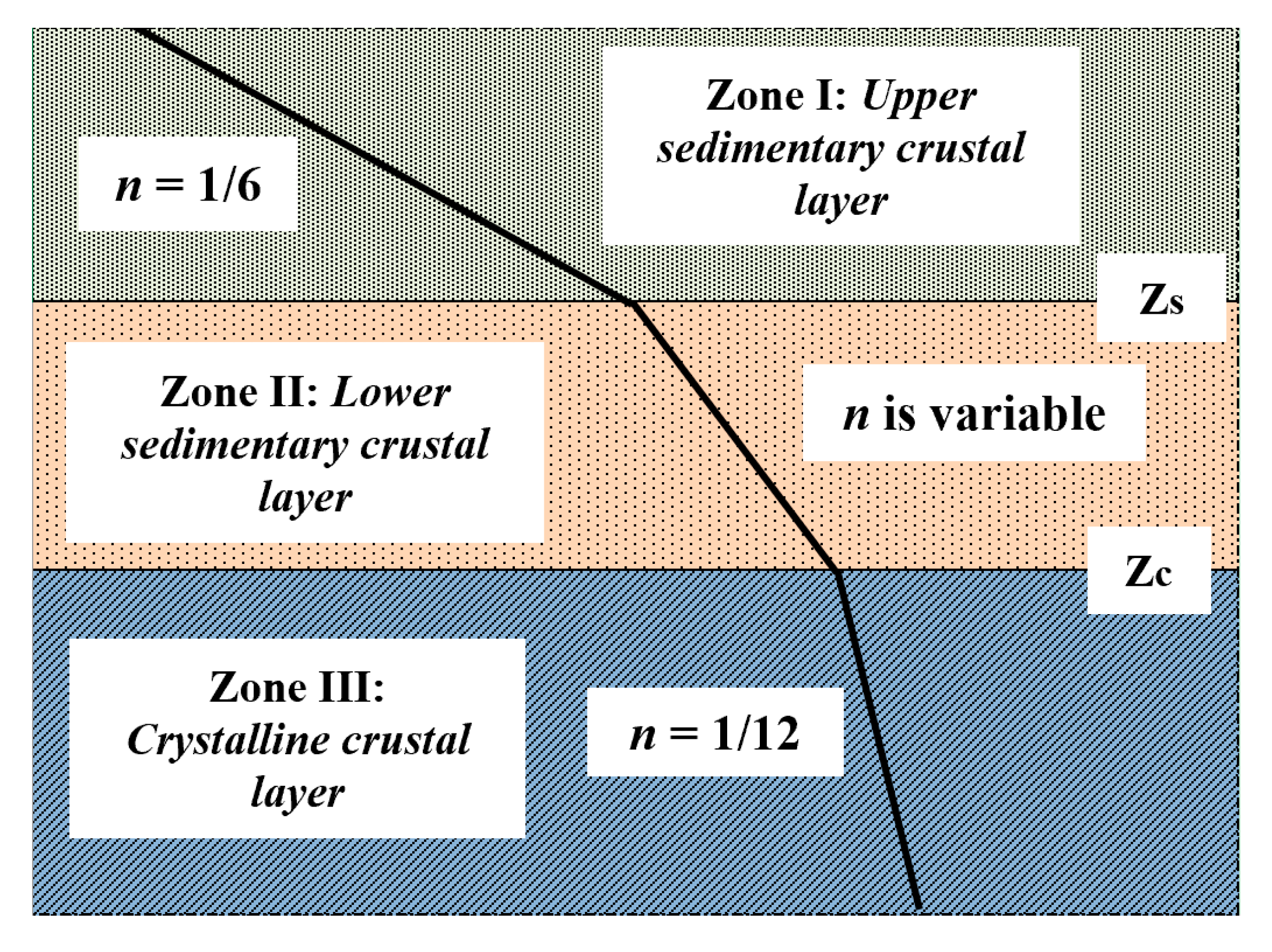
Figure 2.
The proposed VS/VP model alongside various recording data.

Figure 3.
Comparison analysis of proposed VS/VP with four selected VS–VP relationship equations.
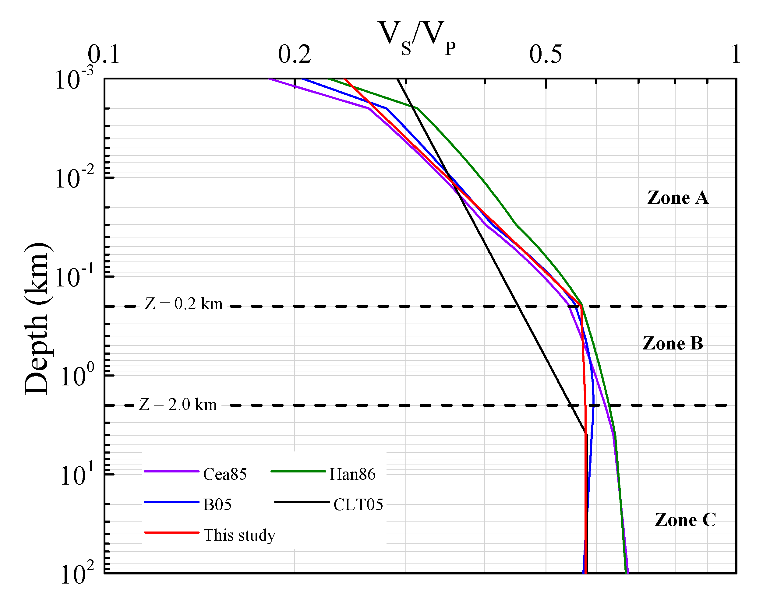
Figure 4.
Illustration of shear-wave velocity profile modeling zone by zone.

Figure 5.
Programming flowchart of the VS profiling model, which is shown in Table 3.
Figure 5.
Programming flowchart of the VS profiling model, which is shown in Table 3.
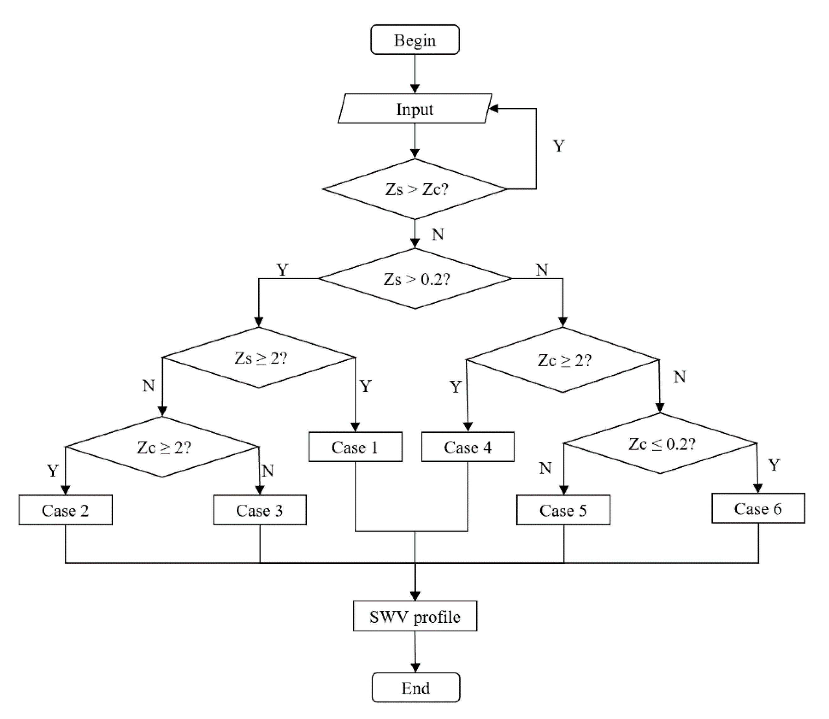
Figure 6.
Location of sampling points in study regions, (a) Melbourne Region; (b) St. Louis Metro Region; (c) Hong Kong Region; (d) Northern Switzerland.
Figure 6.
Location of sampling points in study regions, (a) Melbourne Region; (b) St. Louis Metro Region; (c) Hong Kong Region; (d) Northern Switzerland.
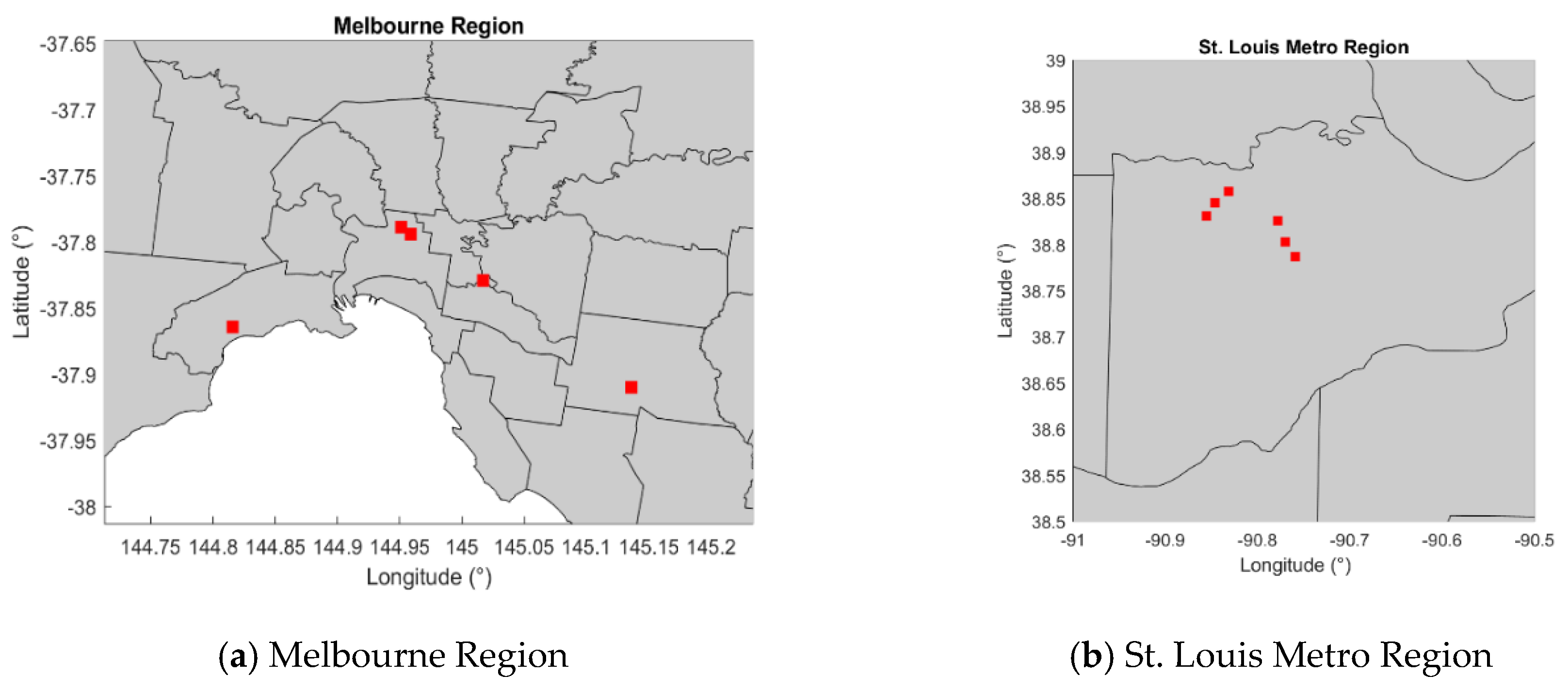
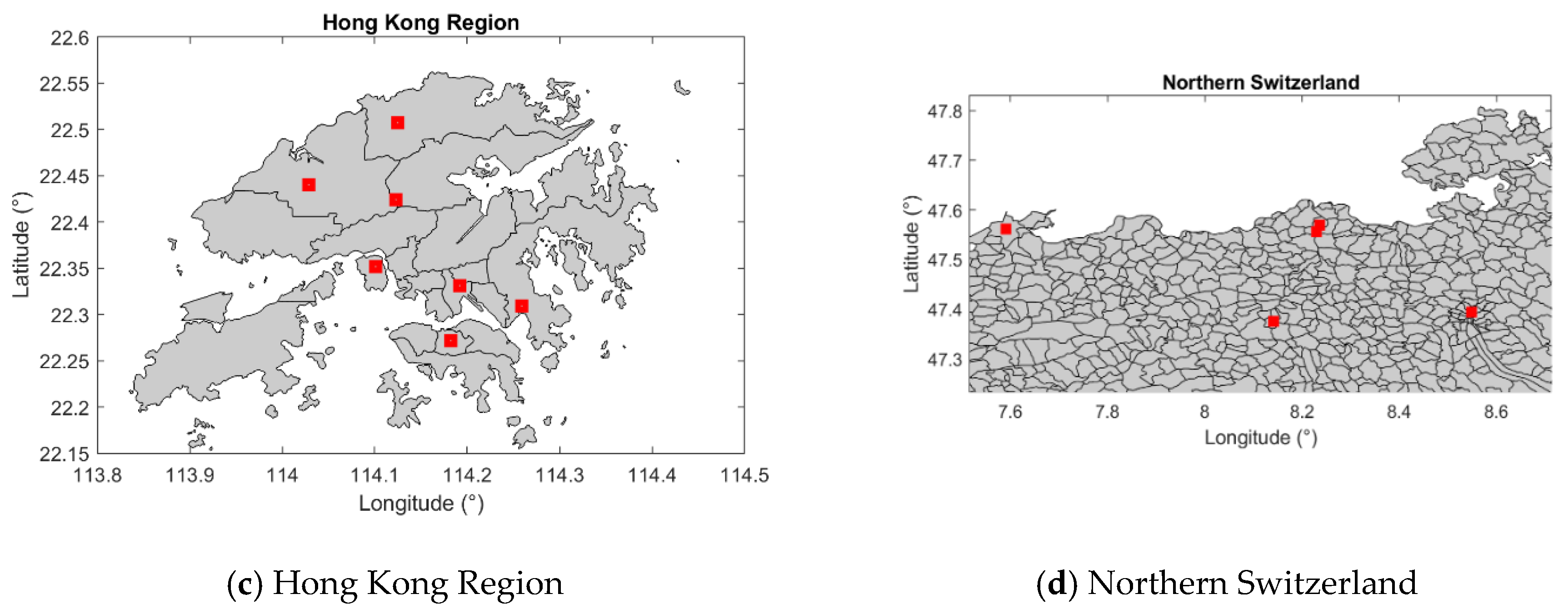
Figure 7.
VS profiles for selected regions for the depth ranging from 0.001 to 50 km, (a) Melbourne Region; (b) St. Louis Metro Region; (c) Hong Kong Region; (d) Northern Switzerland. Dash lines indicate the field measurements; square marker lines indicate the average field measurements; round markers indicate the VS values collected from CRUST1.0.

Figure 8.
Residuals for selected regions, with the depth ranging from 0.001 to 10 km, (a) Melbourne Region; (b) St. Louis Metro Region; (c) Hong Kong Region; (d) Northern Switzerland. Residual is defined as the discrepancy between the model estimate and average field measurement at each depth. The solid line indicates the average residual for all depth of each model.
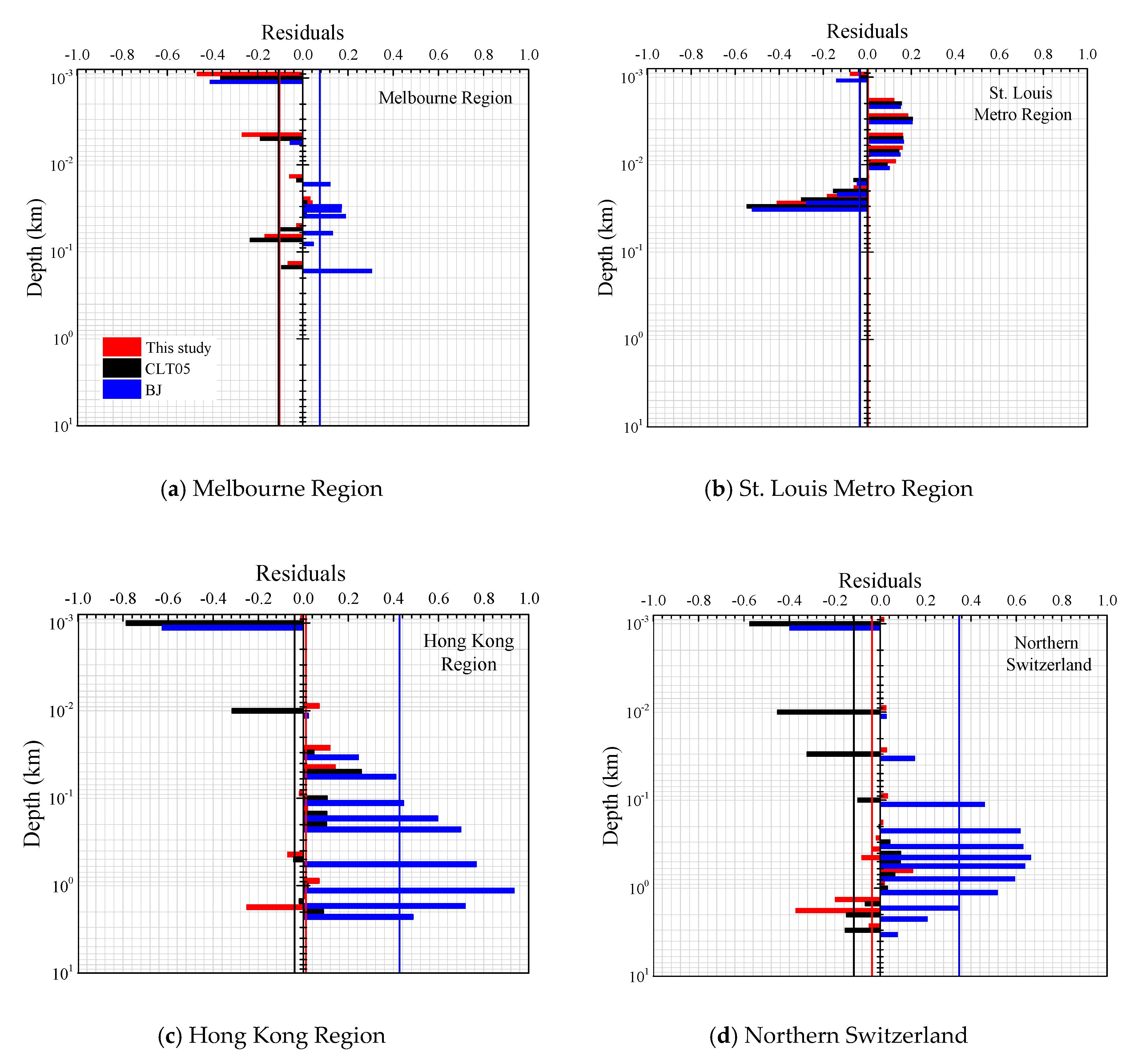
Figure 9.
Upper-crust amplification for selected regions. GR site and GHR site are obtained from [2] and used for general comparison, for the frequency ranging from 0.1 to 100 Hz.
Figure 9.
Upper-crust amplification for selected regions. GR site and GHR site are obtained from [2] and used for general comparison, for the frequency ranging from 0.1 to 100 Hz.

Table 1.
Field measurement data used for regression analysis.
| Region | Data Acquisition Method | No. of Recordings | Citations |
|---|---|---|---|
| WNA | Seismic refraction data | 10 | [3] |
| CENA | Seismic refraction data | 4 | [3] |
| Eastern China | Seismic refraction data | 4 | [3] |
| Hong Kong | Engineering borehole data | 14 | [30,31] |
| Central California | Engineering borehole data | 3 | [32] |
| Michigan Basin | Vertical seismic profiling experiment | 39 | [33] |
| Southern California | Qualitative analysis of near-source data | 3 | [34] |
| Eastern Sierra Nevada | Seismic refraction data | 7 | [27] |
| South-central Alaska | Seismic refraction and reflection survey and laboratory experiment | 7 | [35] |
| California | Engineering borehole data | 69 | [36] |
| San Francisco Bay Area | Seismic refraction data | 5 | [37] |
| Gansu, China | Seismic refraction data | 6 | [38] |
| Sichuan, China | Seismic refraction data | 4 | [39] |
| Tibet, China | Seismic refraction data | 3 | [39] |
| Kilauea caldera | In situ estimate | 3 | [40] |
| Indian subcontinent | Seismic cross-hole tests | 9 | [41] |
| ENA | Engineering borehole data | 3 | [2] |
Table 2.
VS–VP relationship equations used for comparison purpose.
| Equations | Citations |
|---|---|
| VS = 0.862VP − 1.172 | [42] |
| VS = 0.794VP − 0.787 | [43] |
| VS = 0.7858 − 1.2344VP +0.7949VP2 − 0.1238VP3 + 0.0064VP4 | [20] |
| VS = 0.58 × (Z/4)1/12VP, Z ≤ 4 km VS = 0.58VP, Z > 4 km | [3] |
Table 3.
The functional forms of VS profile model in this study.
| Case | Depth Range (km) | VS (km/s) | Zone |
|---|---|---|---|
| Case 1 (ZS ≥ 2) | 0 < Z ≤ 0.2 | VS0.03 (Z/0.03)0.3297 | IA |
| 0.2 < Z ≤ 2 | VS0.2 (Z/0.2)0.1732 | IB | |
| 2 < Z ≤ ZS | VS2 (Z/2)0.1667 | IC | |
| ZS < Z ≤ ZC | VSZC (Z/ZC)n | II | |
| ZC < Z | VS8 (Z/8)0.0833 | IIIC | |
| Case 2 (0.2 < ZS < 2 ≤ ZC) | Z ≤ 0.2 | VS0.03 (Z/0.03)0.3297 | IA |
| 0.2 < Z ≤ ZS | VS0.2 (Z/0.2)0.1732 | IB | |
| ZS < Z ≤ ZC | VSZC (Z/ZC)n | II | |
| ZC < Z | VS8 (Z/8)0.0833 | IIIC | |
| Case 3 (0.2 < ZS < ZC ≤ 2) | 0 < Z ≤ 0.2 | VS0.03 (Z/0.03)0.3297 | IA |
| 0.2 < Z ≤ ZS | VS0.2 (Z/0.2)0.1732 | IB | |
| ZS < Z ≤ ZC | VSZC (Z/ZC)n | II | |
| ZC < Z ≤ 2 | VS2 (Z/2)0.0899 | IIIB | |
| 2 < Z | VS8 (Z/8)0.0833 | IIIC | |
| Case 4 (ZS < 0.2 < 2 ≤ ZC) | 0 < Z ≤ ZS | VSZI (Z/ZI)0.3297 | IA |
| ZS < Z ≤ ZC | VSZC (Z/ZC)n | II | |
| ZC < Z | VS8 (Z/8)0.0833 | IIIC | |
| Case 5 (ZS < 0.2 < ZC ≤ 2) | Z ≤ ZS | VSZI (Z/ZI)0.3297 | IA |
| ZS < Z ≤ ZC | VSZC (Z/ZC)n | II | |
| ZC < Z ≤ 2 | VS2 (Z/2)0.0899 | IIIB | |
| 2 < Z | VS8 (Z/8)0.0833 | IIIC | |
| Case 6 (ZC ≤ 0.2) | 0 < Z ≤ ZS | VSZI (Z/ZI)0.3297 | IA |
| ZS < Z ≤ ZC | VSZC (Z/ZC)n | II | |
| ZC < Z ≤ 0.2 | VS0.2 (Z/0.2)0.2463 | IIIA | |
| 0.2 < Z ≤ 2 | VS2 (Z/2)0.0899 | IIIB | |
| 2 < Z | VS8 (Z/8)0.0833 | IIIC |
(ZS and ZC are the thickness of upper sediment layer and total sediment layers respectively; VS0.03, VS0.2, VS2, and VS8 are the VS value at the depth of 0.03, 0.2, 2, and 8 km; VSZS and VSZC are the VS value at the depth of ZS and ZC respectively. ZI = min (ZS, 0.03)).
Table 4.
Geological location of sampling points for the study regions.
| Region | Location Name | Latitude | Longitude |
|---|---|---|---|
| Melbourne Region | Trinity College | −37.79 | 144.96 |
| Royal Park | −37.79 | 144.95 | |
| Monash Uni | −37.91 | 145.14 | |
| Burnley | −37.83 | 145.02 | |
| Altona | −37.86 | 144.82 | |
| St. Louis Metro Region | Lake St Louis Blvd. interchange | 38.80 | −90.77 |
| US 61 west service road | 38.83 | −90.86 | |
| Parr Road east side | 38.86 | −90.83 | |
| Guthrie Road east side | 38.83 | −90.78 | |
| Lake St. Louis Blvd. west side | 38.79 | −90.76 | |
| Mexico Rd | 38.85 | −90.85 | |
| Hong Kong Region | Yuen Long | 22.44 | 114.03 |
| Tsing Yi | 22.35 | 114.10 | |
| Sheung Shui | 22.51 | 114.13 | |
| Happy Valley | 22.27 | 114.18 | |
| Tseung Kwan O | 22.31 | 114.26 | |
| Kowloon City | 22.33 | 114.19 | |
| New Territories | 22.42 | 114.12 | |
| Northern Switzerland | Boettstein | 47.57 | 8.24 |
| Beznau | 47.56 | 8.23 | |
| Schafisheim | 47.38 | 8.14 | |
| Basel | 47.56 | 7.59 | |
| Zentralschweiz | 47.39 | 8.55 |
Table 5.
Parameters of the VS profile mode ling in this study.
| Region | Melbourne Region | St. Louis Metro Region | Hong Kong Region | Northern Switzerland |
|---|---|---|---|---|
| ZS (km) | 0.05 | 0.5 | 0.001 | 0.001 |
| ZC (km) | 4.0 | 4.0 | 1.0 | 0.62 |
| VSZI (km/s) | 1.1 | 2.0 | 1.50 | 1.10 |
| VS2 (km/s) | / | / | 2.60 | 2.70 |
| VS8 (km/s) | 3.5 | 3.6 | 3.5 | 3.6 |
| n | 0.21 | 0.22 | 0.049 | 0.10 |
| VS30 (km/s) * | 0.96 | 0.69 | 1.61 | 1.37 |
(* VS30 value is obtained from the average field measurement for each region).
© 2020 by the authors. Licensee MDPI, Basel, Switzerland. This article is an open access article distributed under the terms and conditions of the Creative Commons Attribution (CC BY) license (http://creativecommons.org/licenses/by/4.0/).
Share and Cite
MDPI and ACS Style
Tang, Y.; Xiang, X.; Sun, J.; Zhang, Y. A Generic Shear Wave Velocity Profiling Model for Use in Ground Motion Simulation. Geosciences 2020, 10, 408. https://doi.org/10.3390/geosciences10100408
AMA Style
Tang Y, Xiang X, Sun J, Zhang Y. A Generic Shear Wave Velocity Profiling Model for Use in Ground Motion Simulation. Geosciences. 2020; 10(10):408. https://doi.org/10.3390/geosciences10100408
Chicago/Turabian StyleTang, Yuxiang, Xinmei Xiang, Jing Sun, and Yongshan Zhang. 2020. "A Generic Shear Wave Velocity Profiling Model for Use in Ground Motion Simulation" Geosciences 10, no. 10: 408. https://doi.org/10.3390/geosciences10100408
Note that from the first issue of 2016, this journal uses article numbers instead of page numbers. See further details here.