Comparison of Two Ensemble-Kalman Filter Based Methods for Estimating Aquifer Parameters from Real 3-D Hydraulic and Tracer Tomographic Tests

Abstract

Pumping and tracer tests are site-investigation techniques frequently used to determine hydraulic conductivity. Tomographic test layouts, in which multiple tests with different combinations of injection and observation wells are performed, gain a better insight into spatial variability. While hydraulic tomography has repeatedly been applied in the field, tracer tomography lags behind. In a previous publication, we presented a synthetic study to investigate whether the ensemble Kalman Filter (EnKF) or the Kalman Ensemble Generator (KEG) performs better in inverting hydraulic- and tracer-tomographic data. In this work, we develop an experimental method for solute-tracer tomography using fluorescein as a conservative tracer. We performed hydraulic- and tracer-tomographic tests at the Lauswiesen site in Germany. We analyzed transient drawdown and concentration data with the EnKF and steady-state hydraulic heads and mean tracer arrival times with the KEG, obtaining more stable results with the KEG at lower computational costs. The spatial distribution of the estimated hydraulic conductivity field agreed with earlier descriptions of the aquifer at the site. This study narrows the gap between numerical studies and field applications for aquifer characterization at high resolution, showing the potential of combining ensemble-Kalman filter based methods with data collected from hydraulic and solute-tracer tomographic experiments.

1. Introduction

Pumping and tracer tests are frequent site-investigation techniques used to determine aquifer parameters, notably hydraulic conductivity (K). The data retrieved with such tests in their conventional layout yield average characteristics of the subsurface material being investigated and usually give limited information of subsurface heterogeneity. However, resolving the spatial variability in hydraulic conductivity is critical, for example in the design of efficient groundwater remediation systems, in which solute transport is partially controlled by small-scale variations in hydraulic properties [1].

The limitations of conventional hydraulic testing have motivated the development of more sophisticated methods such as tomographic aquifer experiments, in which large datasets representative of different parts (and different processes) of the subsurface can be collected. The idea behind a tomographic aquifer test is to sequentially stress the aquifer at multiple isolated sections and measure the response at many observation points. The observations are then inverted to estimate aquifer parameters. The most common application of an aquifer tomographic method is hydraulic tomography, which involves a sequence of pumping tests with multiple injection/extraction wells and many observation locations to monitor hydraulic head changes. Hydraulic tomography has been applied successfully in theoretical, laboratory, and field studies [2,3,4,5,6,7,8,9,10,11,12,13,14,15,16,17,18,19,20,21,22,23,24,25,26,27], however, the diffusive nature of groundwater-flow limits the information contained in the observed data, no matter how sophisticated the chosen test layout is [28,29,30,31]. Recent studies suggest that this limitation can be overcome by integrating data of different types (e.g., hydraulic head and tracer concentrations) in parameter estimation. The different sensitivity patterns of each data type help improve the resolution and reduce the uncertainty of the estimate [32,33,34,35].

The relevance of tracer data for aquifer characterization has motivated the adaptation of traditional tracer tests into a tomographic layout. In analogy to hydraulic tomography, tracer tomography involves a series of tracer tests with tracer injection at different locations or in different depths of the aquifer. The concept of tracer tomography has been investigated mainly in numerical [34,35,36,37,38,39] and laboratory [33,40] studies. The logistic effort and associated costs have hindered its field application in real aquifers. Doro et al. [41] presented a field method to perform tomographic tracer tests and showed its viability with a field experiment performed at the hydrogeological research site Lauswiesen, in Germany. Somogyvári and Bayer [42] obtained a hydraulic-conductivity tomogram based on tracer data collected during a field tracer tomography experiment at the Widen field site, in Switzerland. Both studies used heat as tracer.

The datasets retrieved from combined tomographic experiments require inverse models that can use the information at reasonable computational costs. Different inverse methods have been proposed [43,44,45], but the large datasets recorded and the high spatial resolution aimed for the estimated parameter fields limit the application of many approaches. Gauss–Newton methods, for example, require the sensitivity of all observations with respect to all parameters. This may be achieved by solving as many adjoint problems as there are measurements [46,47,48,49]. This approach, however, imposes prohibitive computational costs if a highly discretized model and many observations are used.

An efficient alternative is data assimilation, in which real and simulated observations at the current state of a system are merged, the model states and/or parameters are corrected to minimize their differences, model simulations are run forward in time until new observations are available and the differences are evaluated again. A particularly popular data assimilation method in hydrogeology is the ensemble Kalman filter [50], due to its simplicity in implementation and efficiency for correcting (or updating) model states and/or parameters, for which sensitivities are not explicitly calculated. The covariance matrices needed in the update step are evaluated by ensemble-averaging within Monte Carlo simulations. The premise is that the efficiency of data assimilation methods in updating model parameters and/or states may enable resolving aquifer heterogeneity at higher resolutions, given that enough information is available. As the main objective of aquifer tomographic tests is to provide comprehensive information about subsurface heterogeneity, it seems a natural choice to explore the performance of data assimilation schemes in the estimation of aquifer parameters with tomographic data sets. Although different applications of ensemble-Kalman filter based methods in groundwater problems can be found in the literature [51,52,53,54,55,56,57], their application to data from combined hydraulic and tracer tomographic experiments has not yet been reported.

This work is the follow up to a synthetic study [58] on the application of two data assimilation methods to the estimation of spatially distributed hydraulic conductivity: (1) the Ensemble Kalman Filter (EnKF) and (2) the Kalman Ensemble Generator (KEG). In the preceding synthetic study [58], we showed that the EnKF and KEG are well-fitted for the estimation of spatially distributed hydraulic conductivity fields from hydraulic- and tracer-tomographic data. In this paper, we applied these techniques to field experiments and to the estimation of aquifer parameters with the data collected in real tomographic aquifer tests.

The approach for the assimilation of field data follows the methods presented in the synthetic study. We used the same numerical models to simulate groundwater flow and solute transport but extended the problem to three spatial dimensions. To minimize repetition, we refer the reader to the previous paper [58] and the references therein for a more in-depth description of the theory behind groundwater flow, solute transport, and the application of ensemble-Kalman filter based methods to groundwater problems. The experimental work presented here was applied at the hydrogeological research site Lauswiesen in Germany.

This work is motivated by the constant evolution of modern measurement devices that have led to better, smaller, and affordable sensors. Unlike previous field applications [41,42], in which heat was used as tracer, the experimental setup developed in this work uses fluorescein as conservative tracer, avoiding issues related to the high diffusivity of heat, density and viscosity effects caused by changes in water temperature, and the technical difficulties associated with the injection of water for long time periods at a temperature different than that of the ambient groundwater.

Like in the synthetic study [58], we applied the standard update scheme of the EnKF to assimilate transient drawdown data. In this scheme the parameters (and/or model states) are updated by evaluating the model performance from the current state to one step forward in time. For the assimilation of tracer concentrations, we applied a restart scheme of the EnKF, in which parameters are updated in the analysis of a time step and solute transport is resimulated from the initial time until the next available measurement time step [59,60,61,62]. Although computationally more demanding, the restart scheme is necessary to honor mass conservation and consistency between hydraulic parameters and model states during transport simulations [58]. In contrast, parameter updating with the KEG was performed by assimilating all available information simultaneously, with an iterative approach in which the same data are reused to update all ensemble members. The update scheme of the KEG requires full forward simulations, posing prohibitive computational costs for three-dimensional transient groundwater flow and solute transport simulations of finely discretized numerical models. To reduce the computational burden, we directly solved for steady-state flow and the first two temporal moments of tracer concentration and used only steady-state hydraulic heads and mean breakthrough times as data for the update.

We estimated effective aquifer parameters by type-curve matching of analytical and semianalytical solutions of the groundwater flow [63,64,65] and advection–dispersion equations [66,67]. This information was considered, together with information from previous investigations, in the geostatistical models applied for the generation of the ensemble of parameters.

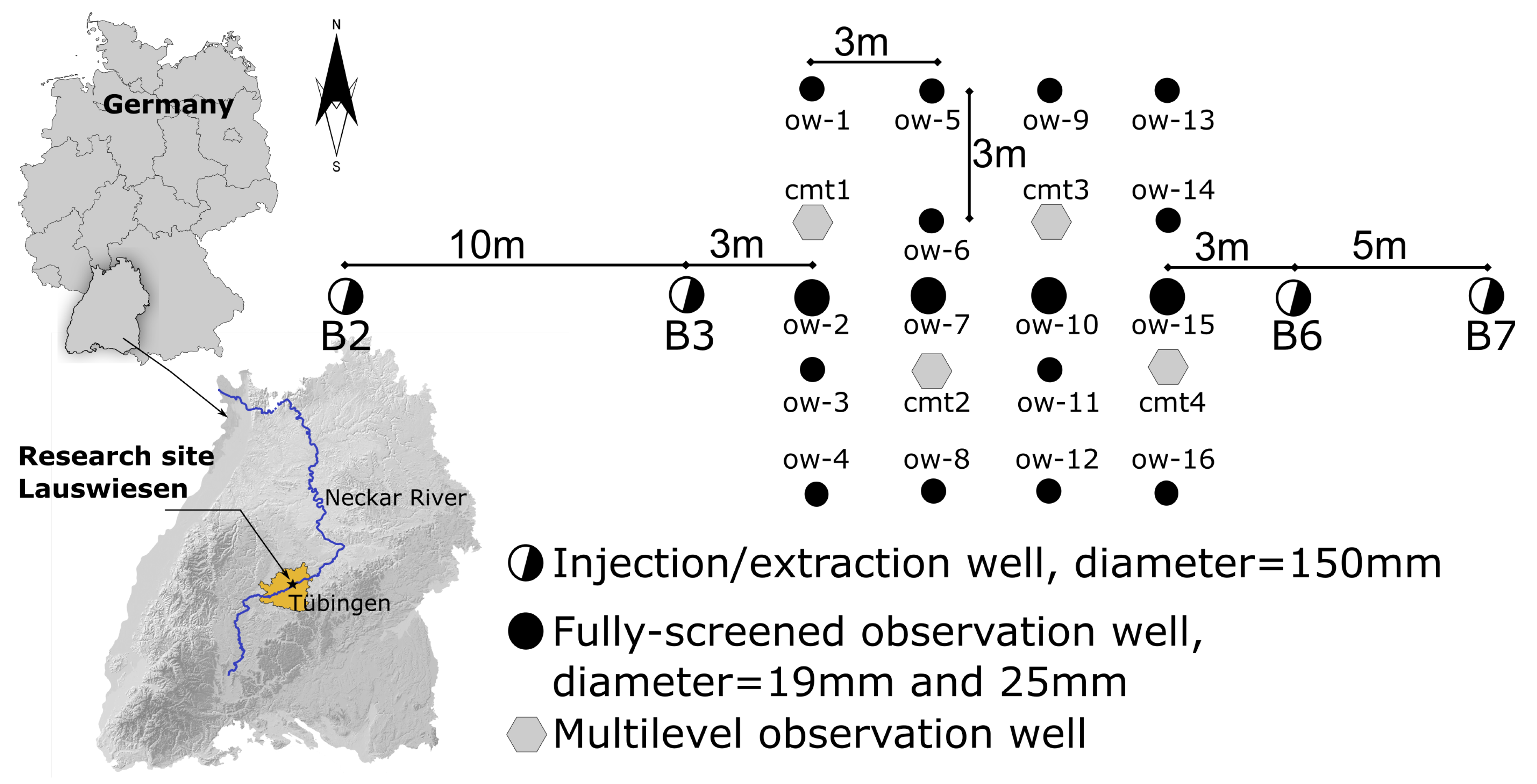
The work is structured as follow. Section 2 is dedicated to the underlying theory and governing equations describing groundwater flow and solute transport. Section 3 summarizes the theory of ensemble-Kalman filter based methods for parameter estimation. Section 4 describes the general hydrogeological setting of the aquifer at the research field site Lauswiesen and the experimental design of the aquifer tomographic experiments. Section 5 presents the dataset obtained with the field experiments and describes the general methodology applied to denoise and process the raw data. Section 6 contains a description of the numerical models used to simulate the aquifer tomographic experiments and the settings of the EnKF and KEG applied for the assimilation of the field data. Section 7 presents the results of the parameter estimation using both ensemble-Kalman filter based methods. This work ends in Section 8 with conclusions, a discussion of the limitations of the proposed methodology, and recommendations to improve solute-tracer tomography on the field scale.

2. Governing Equations

We consider the spatial field of isotropic hydraulic conductivity K($\mathbf{x}$) [$L{T}^{-1}$] and the transient hydraulic-head field h(t,$\mathbf{x}$) [L] as described by the groundwater flow equation:

$$S_0\frac{\partial h}{\partial t}-\nabla ·\left(K\nabla h\right)=W_0$$

(1)

subject to:

$$h=h_{0}att=t_0\forall \mathbf{x}$$

(2)

$$h=h_{in}at{\Gamma }_{in}\forall t$$

(3)

$$h=h_{out}at{\Gamma }_{out}\forall t$$

(4)

$$\widehat{\mathbf{n}}·\left(-K\nabla h\right)=q_{fix}\left(x\right)at{\Gamma }_{no}\forall t$$

(5)

in which $\mathbf{x}$ [L] is the vector of spatial coordinates, $S{}_0$ [$L^{-1}$] is the specific storage coefficient, t [T] denotes time, $t_0$ [T] refers to the initial time, $W_0$ [$T^{-1}$] describes volumetric sources or sinks (e.g., injection/extraction wells), ${\Gamma }_{in}$ and ${\Gamma }_{out}$ are the Dirichlet boundaries at the in- and outflow of the domain, respectively, and ${\Gamma }_{no}$ represents the Neumann boundaries with defined normal flux $q_{fix}$ [$L{T}^{-1}$]. $\widehat{\mathbf{n}}$ is the unit vector normal to the boundary pointing outwards. $h_0$[L], $h_{in}$[L], and $h_{out}$[L] denote the initial and boundary values of hydraulic head, and the specific discharge $\mathbf{q}$ [$L{T}^{-1}$] follows Darcy’s law ($\mathbf{q}=-K\nabla h$).

We also assume solute transport described by the dual-domain advection–dispersion equation, which separates the pore space of an aquifer into mobile and immobile continuous domains and assumes that the mass transfer between the two domains is proportional to the corresponding concentration difference [68,69]:

$$n_m\frac{\partial c_m}{\partial t}+n_{im}\frac{\partial c_{im}}{\partial t}+\nabla ·\left(\mathbf{q}{c}_m-n_m\mathbf{D}\nabla c_m\right)=0$$

(6)

$$\frac{\partial c_{im}}{\partial t}={\lambda }_{mt}\left(c_m-c_{im}\right)$$

(7)

subject to:

$$c_m=c_{im}=0att=0\forall \mathbf{x}$$

(8)

$$c_m=c_{in}at{\Gamma }_{in,c}\forall t$$

(9)

$$\widehat{\mathbf{n}}·\left(\mathbf{D}\nabla c\right)=0at\Gamma \backslash {\Gamma }_{in,c}\forall t$$

(10)

in which $c_m$ [$M{L}^{-3}$] and $c_{im}$ [$M{L}^{-3}$] refer to the tracer concentrations in the mobile and immobile domains, respectively, $n_m$ [$L^3{L}^{-3}$] and $n_{im}$ [$L^3{L}^{-3}$] are the corresponding porosities, $\mathbf{D}$ [$L^2{T}^{-1}$] is the dispersion tensor, ${\lambda }_{mt}$ [$T^{-1}$] is the first-order solute exchange coefficient between the mobile and immobile zones, $\Gamma$ represents all domain boundaries, and $c_{in}$ [$M{L}^{-3}$] is a known concentration along the inflow boundary ${\Gamma }_{in,c}$. If the mobile porosity equals the total porosity and the immobile porosity is set to zero, the model described by Equations (6) and (7) simplifies to the classical advection–dispersion equation. The seepage velocity $\mathbf{v}$ [$L{T}^{-1}$] is defined as the specific discharge divided by the porosity ($\mathbf{v}=\mathbf{q}/n$).

Additionally, we consider temporal moments of tracer concentration, which can be computed by temporal-moment generating equations [70]:

$$\mathbf{q}·\nabla \left(m_k^c-n_m\mathbf{D}\nabla m_k^c\right)=n_{m}k{m}_{k-1}^c+n_{im}k{m}_{k-1}^{c_{im}}$$

(11)

$$-k{m}_{k-1}^{c_{im}}=\lambda \left(m_k^c-m_k^{c_{im}}\right)$$

(12)

in which $m_k^c$ is the k-th raw temporal moment of the tracer concentration c. Equations (11) and (12) imply that the zeroth moments $m_0^c$ and $m_0^{c_{im}}$ of the mobile and immobile concentrations are identical, and the first moment of the mobile concentration does not differ between the standard advection–dispersion model and the dual-domain case with two porosities. In our analysis, we used mean tracer arrival times, that is, the ratio of the first over the zeroth temporal moment of concentration, rather than the moments themselves as observations.

3. Parameter Estimation with Ensemble-Kalman Based Methods

We applied the same ensemble-Kalman filter based methods for parameter estimation as those used in the synthetic study of the companion paper [58]: the Ensemble Kalman Filter (EnKF) and the Kalman Ensemble Generator (KEG). Ensemble-Kalman filter based methods are recursive processes with a forecast-update cycle defined by Equation (13) (forecast) and Equation (14) (update) [71]. Both the EnKF and KEG share the same underlying theory and differ only in the way observations are analyzed.

$$\begin{array}{ccc}\hfill {\mathbf{y}}_t^{sim,i}& =& \mathbf{f}\left({\mathbf{p}}_{t-1}^i\right)\hfill \end{array}$$

(13)

$$\begin{array}{ccc}\hfill {\mathbf{p}}_c^i& =& {\mathbf{p}}_u^i+\beta {\mathbf{Q}}_{py}{\left({\mathbf{Q}}_{yy}+\mathbf{R}\right)}^{-1}\left({\mathbf{y}}^{obs}-\left({\mathbf{y}}^{sim,i}-{\mathit{ϵ}}^i\right)\right)\hfill \end{array}$$

(14)

in which $i=1,2,\dots ,N_{ens}$ is the ensemble index, and $N_{ens}$ is the number of ensemble members, $\mathbf{f}$ is the model that simulates the model states ${\mathbf{y}}^{sim}$ (e.g., drawdown or concentrations) for given parameters (e.g., hydraulic conductivity) and preceding states $\mathbf{p}$, and t [T] is the time index, ${\mathbf{y}}^{obs}$ and ${\mathbf{y}}^{sim,i}$ are the real and simulated observations, respectively. Measurement noise $\mathit{\epsilon }$ drawn from a multi-Gaussian probability distribution with zero mean and covariance matrix $\mathbf{R}$ is added to the simulated observations [72]. The subscripts u and c refer to the unconditional and conditional state and/or parameter vector $\mathbf{p}$, respectively, and $\beta$ is a damping factor that ranges between 0 and 1, which reduces the step size of parameter updates. The matrices ${\mathbf{Q}}_{yy}$ ($N_{obs}\times N_{obs}$) and ${\mathbf{Q}}_{py}$ ($N_{par}\times N_{obs}$) are the auto-covariance matrix of modeled observations and the cross-covariance matrix between model parameters and modeled observations, respectively, computed from the model ensemble. $N_{par}$ and $N_{obs}$ refer to the number of parameters and available observations, respectively.

We applied the EnKF with a standard update, damping, and normal-score transformations to assimilate transient hydraulic data, whereas the restart EnKF scheme was implemented without data transformations for concentrations. The normal-score transformation, or Gaussian anamorphosis, is a univariate transformation that modifies the marginal distributions of the variables to standard normal distributions without changing the statistical dependence and thus without ensuring multi-Gaussianity after the transformation. We built an individual transformation function for each measurement location and applied it to both the perturbed modeled observations ($y_{sim,i}+{\mathit{ϵ}}_i$) and the corresponding reference observation $y_{obs}$ [51,73]. In the KEG, we updated parameters by assimilating all observations simultaneously, as it is regularly done in a batch calibration. This scheme follows an iterative approach, in which the same data are reused to update those ensemble members for which the likelihood of the data does not meet an acceptance criterion. In the application of the KEG, we solved only for steady-state flow and the zeroth and first temporal moments of tracer concentration and used the steady-state heads and mean breakthrough times as data. Neither damping nor data transformation were applied during parameter updating with the KEG.

4. Field Site and Test Design

4.1. Hydrogeological Research Site Lauswiesen

The research site Lauswiesen is located in a flat area of the Neckar Valley, east of Tübingen, southwest Germany (Figure 1). The aquifer at the site consists of 8 m to 9 m thick gravel with small amounts of sand (∼10%) and fines (<10%). It is overlain by about 2 m of alluvial fines and underlain by low-conductive claystones of the upper Triassic (Bunte Mergel, Steigerwald to Mainhardt formations). The depth to groundwater is approximately 4 m, defining an unconfined system with an ambient hydraulic gradient between 0.2% to 0.3% to the northeast. Strong variations in the main flow direction are induced by water level changes of River Neckar.

Previous field investigations report a mean hydraulic conductivity value of the aquifer at Lauswiesen of $3\times {10}^{-3}$ ms${}^{-1}$ [25,41,74,75,76,77,78,79,80,81], which is a typical value for deposits dominated by gravel sheets. Extensive direct-push injection-logging and direct-push slug-test field campaigns identified two major aquifer layers, a highly conductive and relatively homogeneous upper unit and a less conductive and more heterogeneous lower layer [82]. These results are supported by fitting multilevel breakthrough curves using a two-layer model [83]. A fitted 3-D dual-domain flow and transport model indicated a mean porosity value of about 26%, with only ∼2% being mobile [25].

The wells used in the present tomographic tests cover an area of about 30 m × 10 m (see Figure 1) and include four fully-screened wells (B-wells) with a diameter of 150 mm, aligned with the main natural groundwater flow direction. Between wells B3 and B6, a total of 20 observation wells are distributed in a $5\times 4$ regular grid. Observation wells cmt1 to cmt4 are multilevel wells [84] with six depth-discrete observation ports each, embedded in a high-density polyethylene (HDPE) multichannel tubing with a diameter of 19 mm. All other observation wells (ow-wells) are fully-screened with a diameter of 25 mm. Overall, a total of 40 observation points were available for monitoring hydraulic head and tracer concentrations. The possibility to retrieve both depth-integrated and multilevel measurements may provide valuable information to represent many important features required to model three-dimensional transport processes [78].

4.2. Test Design

Figure 2 sketches the main details of the experimental design. To constrain the tracer injection to a specific depth-range of the aquifer, a multilevel injection system was installed at well B3, generating three independent injection sections. Throughout the tests, water was injected simultaneously into all three sections, while the tracer injection was restricted to a single section per test. To enforce horizontal flow, water injection was adjusted such that the injection rate in each segment was approximately proportional to the transmissivity of that section. To compute these transmissivities, vertical variations of hydraulic conductivity were taken from previous borehole flowmeter tests [77]. To prevent tracer re-entering the system, extracted water was released more than 40 m downstream, close to the river banks of River Neckar.

The tomographic experiment itself consisted of a series of tracer tests with the injection of ∼1 g of the conservative tracer fluorescein, at one of the three isolated sections of well B3 (injection at the middle section is exemplified in Figure 2). The tracer was injected only after steady-state flow was achieved. Tracer injection times lasted less than one minute, and in comparison with the overall test times (>6 h) a (Dirac) pulse injection was assumed. The steady-state flow field was maintained throughout the entire duration of each individual tracer test. To achieve a tomographic layout, the tracer experiments were repeated after changing the tracer injection interval. Prior to a subsequent experiment, the system was left under natural conditions for at least one day, providing the remnant tracer more time to be flushed out of the domain.

All tracer tests discussed in this work were performed with a forced-gradient flow field in a nested-cell setup. This four-well system, originally suggested for in-situ remediation [85], was implemented in a numerical studies [35,58] within the framework of synthetic thermal and solute tomographic tracer tests, respectively, and implemented at the Lauswiesen field site in tomographic heat-tracer experiments [41]. In the nested-cell flow system, a stable local artificial ambient flow field is achieved with high extraction and injection rates applied at the outer well pair (here wells B2 and B7). The inner well pair (here wells B3 and B6) is then used to create an inner nested flow field with lower injection/extraction rates. To enhance tracer recovery rates during the tracer tests, an asymmetric flow setup was adopted by applying higher extraction than injection rates in both well pairs. The benefits of this flow-field design include: a well-focused flow field, a reduction of the test duration due to high hydraulic gradients, a decreased impact of fluctuating boundary conditions, higher tracer recovery rates, and a minimized leakage of tracer into the environment, that is, any tracer bypassing the inner extraction well is collected by the outer extraction well.

Hydraulic head responses to water injection and extraction were measured with up to 14 fiber optic pressure transducers (FISO Technologies Inc., Quebec, QC, Canada, Sensor: FOP-MIV, signal conditions: FPI-HR), with an accuracy of ±1 mm and a sampling frequency of 1 Hz. These pressure sensors and their respective data loggers are schematically represented in blue in Figure 2. Real-time monitoring of hydraulic head changes helped identifying when quasi steady-state flow was achieved. Hydraulic heads were monitored throughout the entire tracer test to detect any disturbance of the flow field. Tracer concentrations were taken with fiber-optic probes, connected to a 19-channel field fluorometer (Hermes Messtechnik, Stuttgart, Germany), marked in Figure 2 in red, with a sampling frequency of 1 Hz. The field fluorometer measures fluorescence intensity as a response to a stimulation with a LED-light source. Light is transmitted back and forth between the observation points and the detector through fiber optics; it has a detection limit that ranges between 3 $\mathsf{\mu }$gL${}^{-1}$–5 $\mathsf{\mu }$gL${}^{-1}$, and the accuracy depends on the internal settings of the device. However, the accuracy of the instrument also depends on, e.g., the setup of the sensor in the well, the quality of the fiber optic cables, or the color of the well screen. For these reasons we decided to use the field fluorometer only as a detector producing a voltage signal. To scale the intensity in mV to concentration values in mgL${}^{-1}$, we collected several groundwater samples at each monitored observation well, measured the concentration in the laboratory, and performed a linear regression between the voltage signal at the time point of sampling and the concentration measured in the lab. We estimate that this procedure leads to an an absolute error of 1 $\mathsf{\mu }$gL${}^{-1}$ and a 5% relative error.

For a better spatial coverage, we performed two tests per injection interval, for which the pressure transducers and fluorosensors were swapped among the available observation wells, leading to a total of six tracer tests. Tracer breakthrough was also recorded at the injection and extraction wells in all tests. The different active observation wells used in each test can be seen in the legends of Figures 6 and 7, where we present the field hydraulic and tracer dataset. For clarity, we labeled each test according to the injection location. The two tests with tracer injection at the top level are referred to as tests 1a and 1b. Tests 2a and 2b and tests 3a and 3b correspond to the experiments with tracer injection at the middle and bottom sections, respectively. We further distinguish between drawdown and concentrations by an additional pumping or tracer label.

Table 1. Summary of the experimental setup of each individual tracer test of the solute-tracer tomography experiment. Top, Mid, and Bot refer to the top, middle, and bottom section generated with the multilevel injection system placed in well B3. Positive flow rates represent injection of water, whereas negative flow rates refer to extraction rates.

Test	Inj.Depth (m)	Tracer	Applied Flow Rates (${\mathit{Ls}}^{-1}$)
	(Level)	Mass(gr)	B2	B3Top	B3Mid	B3Bot	B6	B7
1a	4.0–5.0 (Top)	1.10	5.2	1.6	0.9	0.6	$-2.0$	$-9.0$
1b	4.0–5.0 (Top)	1.15	4.8	2.0	0.87	0.6	$-2.4$	$-9.0$
2a	5.5–6.5 (Mid)	1.10	5.2	1.8	0.9	0.6	$-2.5$	$-9.0$
2b	5.5–6.5 (Mid)	1.20	4.9	2.1	0.81	0.6	$-2.0$	$-9.0$
3a	7.0–8.0 (Bot)	1.10	5.2	1.8	0.9	0.6	$-2.5$	$-9.0$
3b	7.0–8.0 (Bot)	1.15	4.9	2.2	0.82	0.6	$-2.0$	$-8.7$

summarizes each test setup by injection/extraction rates, tracer injection location, and mass of the injected tracer. Small differences in the injection and extraction rates between tests a and b of each injection level and in the mass of the injected tracer were unavoidable and taken into account in the numerical analysis.

5. Data Processing and Preliminary Aquifer Characterization

To increase the signal-to-noise ratio, correct signal shifts and/or remove outliers, background values, and trends introduced by the sensors in the collected dataset, we used smoothing functions and low-pass filters to remove high frequency noise and automated outlier detection algorithms based on the modified Z-scores [86].

To account for the anomalous transport observed at the research site Lauswiesen [25,78], which is characterized by early breakthrough and long tailing, we fitted the generalized inverse Gaussian (GIG) distribution [87] to the tracer data, and used the fitted curve in those cases in which the parametric model and the field data showed a good agreement. The objective of fitting a parametric function to noisy data is to find a smooth curve that follows the trend of the data but is fully characterized by a few parameters. While a parametric model has the disadvantage that it predefines the general shape of the curve, it has the advantage that it can be used for extrapolation, which may be relevant in the estimation of transport parameters using temporal moments. If the fitted curve preserves the main features of the original data, e.g., first arrival, peak, and observed part of tail of a breakthrough curve, it may be considered instead of the actual data. If the main features are not described well enough, they should not be used.

The GIG distribution $f\left(x\right)$ is defined as:

$$f\left(x\right)=\eta \frac{{(a/b)}^{p/2}}{2K_p\left(\sqrt{ab}\right)}{(x-\Delta x)}^{(p-1)}exp\left(-\left(a\right(x-\Delta x)+b/(x-\Delta x\left)\right)/2\right)+\Delta y,\forall x>0$$

(15)

in which $K_p$ is the modified Bessel function of the second kind and order p, and a and b are non-negative parameters. The GIG distribution includes the inverse Gaussian distribution, which is the analytical solution for the 1-D advection–dispersion equation with uniform coefficients, as special case ($p=-1/2$) but adding another coefficient facilitates distributions that are more skewed than the inverse Gaussian. The version of the GIG distribution we present in Equation (15) includes a $\Delta x$ and $\Delta y$ for shifts in both dimensions, accounting for delayed arrival times and background values in the observed signal, and a factor $\eta$ that scales the distribution to the units of the data. These parameters regulate the signal recovery, offsets in the baseline of the online fluorometer, and time shifts. The fitting was performed using nonlinear least squares with the Levenberg–Marquardt algorithm. As an example, Figure 3 shows the raw data and the corresponding fitted distribution for the breakthrough curve measured at extraction well B6 during tracer test 3b. Despite the high noise level in the raw signal (gray line), the resulting fitted curve (black dashed line) is a noise-free breakthrough curve with all relevant features of the original data.

To estimate effective values of hydraulic conductivity and specific storage coefficient, we fitted the Theis solution [63] to selected drawdown curves, accounting for multiple injection and extraction wells. Even though the aquifer under investigation is an unconfined system, previous investigations have shown that assuming confined conditions is acceptable for the time scales of the current experiments and for pumping tests in which the drawdown is considerably smaller than the thickness of the aquifer. Effective porosities and dispersivities were estimated by fitting a travel-time based semianalytical solution of the advection–dispersion equation (ADE, Equation (6)) [67], to the breakthrough curves measured at extraction wells B6 and B7. The latter can represent one-dimensional advection and dispersion processes, combined with a dual-porosity domain and a first-order mass transfer reaction between the two regions. The analytical solution exists only in the Laplace domain and the final result is obtained via numerical inverse Laplace transformation [88]. Type-curve matching of the Theis solution to the drawdown data was performed using the Nelder–Mead simplex algorithm that evaluates the fit using direct function evaluations, rather than derivatives. We fitted the travel-time based semianalytical solution to the breakthrough curves using the global search algorithm DREAM-ZS, which is an advanced Markov chain Monte Carlo sampler that provides the estimation together with the associated uncertainty bounds [89].

The full processed dataset of the tracer tomography test consists of 52 drawdown curves and 46 breakthrough curves (Figure 4, Figure 5 and Figure 6). Hydraulic head changes observed during test 2a could not be retrieved due to technical problems with the data loggers. We selected 27 characteristic time points from each processed drawdown curve, for both the estimation of effective aquifer parameters with the Theis solution and for model inversion. The number of characteristic points selected from the breakthrough curves varied between 27 and 34 characteristic points, depending on the length of each test.

Hydraulic responses to injection and extraction of water were similar throughout the five tests shown in Figure 4. The small differences between tests were attributed to the slightly different injection and extraction rates applied. For tests 1a and 1b, steady state was achieved after 5000 s, whereas in all other tests steady-state conditions were not observed before 7000 s. Multiple points taken from the steady-state portion of the drawdown curves would not provide additional information for parameter estimation; therefore, the curves were trimmed at the first time point at which steady-state flow was observed at most locations.

Figure 5 shows the tracer breakthrough curves, normalized by the injected mass, measured at extraction wells B6 and B7 during the six tracer tests of the tracer tomography experiment. The tracer was detected in both extraction wells; however, the concentrations observed in well B7 were one order of magnitude smaller than those of well B6. The difference in peak arrival times observed in tests with tracer injection in the same section (e.g., tracer tests 1a and 1b) is attributed to the slightly different pumping rates applied. Please note that the breakthrough curves measured at pumping well B6 during tests 1b and 2a (Figure 5 top) still show some level of noise, which means that it was not possible to fit the GIG parametric function in a satisfactory way and instead the smoothed curve had to be preserved.

The recovered tracer mass was calculated for the breakthrough curves measured at wells B6 and B7 with temporal moments, where the 0th temporal moment $m_0^c$ represents the effective tracer mass (mass per discharge). The recovered tracer mass indicates the reliability of the recorded data. However, the estimation is highly affected by all processing steps required to transform the raw and noisy breakthrough curves into a smooth time series in units of concentration. We estimated a tracer recovery of 87% and 62% for tracer tests 2a and 2b, respectively. The lowest tracer recovery was estimated for tracer test 3b (32%), indicating that the majority of the tracer was lost into ambient flow or remained somewhere in the domain. Disturbances of the steady-state hydraulic field were not observed, and the reason for the low recovered mass could not be identified. A larger measurement uncertainty was assigned to this dataset when it was used for parameter estimation. The overestimation of the recovered mass for tracer tests 1a, 1b, and 3a (115%, 107%, and 117%, respectively) was attributed to complications during water sampling and uncertainties in the laboratory measurements, leading to errors when the data was scaled to units of concentration.

The breakthrough curves measured in all additional observation wells are shown in Figure 6, normalized by the injected mass. The three plots on the left correspond to the first test series (series a), and the plots on the right are the breakthrough curves of the second test series (series b). A visual inspection of all curves reveals that independent of the tracer injection location, the tracer plume was well distributed horizontally and vertically in the investigated area. Breakthrough curves were observed even at the wells located at the corners of the observation well grid (e.g., in wells ow4, ow13, and ow16) and also at different depths of the multilevel observation wells (e.g., in wells cmt1, cmt2, and cmt3). Except for test 1a, tracer concentrations decreased with a shift of the tracer injection towards the bottom of the aquifer. The highest concentrations were measured in the observation point cmt1-3, which is located at a depth of 4m and directly next to the injection well B3. The vertical location of this point coincides with the top tracer injection section. High tracer concentrations were observed at this point also in tests 3a and 3b, indicating a large and fast vertical spread of the plume. Breakthrough curve tailing was accentuated in the tests with tracer injection at the lower sections of the aquifer. This might indicate a higher degree of heterogeneity and zones with lower hydraulic conductivity.

Figure 7 exemplarily illustrates the fitting of the analytical and semianalytical solutions to some drawdown (top) and breakthrough curves (bottom), and Figure 8 summarizes with violin plots the statistical distribution of the estimated aquifer parameters. In addition to the mean and median (solid and dotted black lines in Figure 8, respectively), violin plots show the shape of the full distribution of a dataset.

In general, the Theis model matches well the hydraulic response to the injection and extraction of water and fits the steady-state values observed during the pumping tests. A mean hydraulic conductivity K of $3.2\times {10}^{-3}$ ms${}^{-1}$ was estimated after averaging the individual values calculated for all drawdown curves of all tests. The corresponding violin plot for K (Figure 8, first column) shows that although the majority of the estimated values cluster around the median, the values distribute more or less uniformly across the estimated range. These estimates agree with previous research performed at the research site Lauswiesen [77,80,81,82]. The observed drawdown is representative of the volume of the domain being investigated. This volume expands with pumping time, producing hydraulic responses that are increasingly averaged [90]. This effect is evidenced in the relatively small coefficient of variation (CV) of $46\%$ calculated for the Theis curve derived hydraulic conductivities. We estimated a mean specific storage coefficient $S_o$ of $8.6\times {10}^{-3}$ m${}^{-1}$ which is typical of confined systems. The large variability in the estimation of $S_0$ (CV = 127%) can be seen as an aliasing effect in which unresolved conductivity appears as a variation of aquifer storativity and is a direct consequence of the application of methods derived under the assumption of homogeneity in heterogeneous systems [90,91,92]. The violin plot for $S_0$ (Figure 8, second column) shows that despite the wide range observed in the estimated values of $S_0$, the most probable values of $S_0$ are well grouped near the median.

Figure 7 (bottom) shows the semianalytical model fitted to the breakthrough curves observed at extraction well B6 during tests 2b (gray solid line) and 3b (orange solid line), together with the associated uncertainty bounds (shaded areas) for a $95\%$ confidence interval. The semianalytical model reproduces the overall shape of the observed breakthrough curves well, with the uncertainty bounds covering the measured data at almost every point in the curve. The largest misfits occur at the first arrival and tail of the curves, for which the field data fall outside the uncertainty bounds. This might indicate the unresolved small-scale variability of aquifer heterogeneity by a semianalytical model. Similar fitted curves were obtained for the rest of the breakthrough curves measured at wells B6 and B7 during all additional tests, and the statistics of all the estimated transport parameters (first-order mass transfer coefficient, mobile and immobile porosities, and dispersivity) are shown in the last four columns of Figure 8.

After fitting all breakthrough curves, we estimated a mean mass transfer coefficient (${\lambda }_{mt}$) and longitudinal dispersivity (${\alpha }_l$) of $2.5$ × 10${}^{-6}$ m${}^{-1}$ and 1.3 m, respectively. These estimates are in agreement with values previously reported for the Lauswiesen site [25,78]. We also estimated mean mobile ($n_m$) and immobile ($n_{im}$) phase porosities of $8\%$ and $7.5\%$, respectively. However, the violin plots for the porosities (Figure 8 columns 4 and 5) show that mean porosity values are strongly affected by values close to $28\%$. Although the median is less affected by extreme values, the small median values estimated for the mobile and immobile porosities ($n_m\sim 3\%$ and $n_{im}\sim 2\%$) are unrealistically low. We have found similar mobile porosity values in preceding studies after fitting an analytical solution to tracer data collected at the same field site, but in those studies total porosity values close to $30\%$ were needed to improve transport simulations [25]. To account for the uncertainty observed in the porosity estimates, spatially uniform mobile and immobile porosities were also updated during the assimilation of the tracer data.

6. Numerical Simulations and Parameter Estimation with Ensemble-Kalman Based Methods

6.1. Numerical Implementation of the Real Tomographic Experiments

We updated the spatially distributed hydraulic conductivity with the EnKF using transient hydraulic heads and tracer concentrations and updated the parameters with the KEG using only steady-state hydraulic heads and mean tracer arrival times. For the former we simulated the hydraulic and tracer experiments in HydroGeoSphere Aquanty, Waterloo, ON, Canada, [93], whereas for the latter, the same experiments were simulated with a numerical model implemented in Matlab that directly computes for steady-state heads and solves for temporal moments of the tracer concentration. Both numerical models presented in this work are three-dimensional versions of the 2-D models presented in the companion paper [58].

The grid of the HydroGeoSphere model consists of ∼760,000 nodes forming 725,700 block elements, distributed over 30 layers. The smallest elements ($\Delta x=\Delta y=\Delta z=0.2$ m) were defined in the region where the extraction, injection, and observation wells are located. This area is referred to as area of interest in Figure 9. The elements were coarsened toward the domain boundaries, reaching a maximum element size of 5 m × 5 m × 0.2 m. The extension of the domain was chosen such that pumping-induced effects were minimized at the boundaries, while keeping model run times acceptable.

A similar grid was implemented in the steady-state groundwater flow and temporal-moment transport model implemented in Matlab, with the same model dimensions and a total of 826,560 nodes forming 799,954 block elements, distributed over 80 layers. Solving steady-state simulations is computationally more efficient; hence, we implemented a finer grid in the area of interest than in the transient model, in both the horizontal and vertical directions ($\Delta x=\Delta y=\Delta z=0.1$ m), without causing a relevant increase in computational demands. In this model, the elements were also coarsened toward the domain boundaries, reaching a maximum element size of 5 m × 5 m × 0.1 m.

In both models, the bottom boundary was set to a constant elevation of 0 m and corresponds to the bottom of the aquifer, and the top was defined as a confined layer at a constant elevation of 6 m. Although the aquifer under investigation is an unconfined system, previous investigations have shown that assuming confined conditions is acceptable for the time scales of the current experiments [25]. Constant-head boundaries were defined at the left and right limits of the domain, and no-flux boundaries at the front, back, bottom, and top faces of the model. In all simulations, the constant head value at the left was set to 10 m, and the constant value at the right was adjusted according to the mean ambient hydraulic gradient, estimated with manual water level measurements taken before the beginning of each test.

The injection and extraction wells B2, B6, and B7 were defined as fully-screened wells, covering the whole aquifer thickness. The three isolated injection sections of well B3 were implemented by creating three different wells identified as B3Top, B3Mid, and B3Bot for the top, middle, and bottom sections, respectively. All ow-wells were implemented as observation wells covering the whole thickness of the aquifer, and all cmt-wells were defined as point observations at the corresponding elevation (see Figure 9).

The field settings of the individual tests, e.g., injection and extraction rates, injected mass of tracer and active observation wells (see Table 1), were considered in the corresponding simulations. We simulated groundwater flow and solute transport separately. For transport, the groundwater flow velocity distribution was calculated with an initial steady-state flow simulation, followed by the injection of tracer at the corresponding location. Dual-domain transport was assumed for the transient tracer-test simulations. Figure 9 (bottom) shows an example of a tracer test simulation at the time of tracer injection in the bottom section of well B3.

6.2. Parameter Estimation with the EnKF and KEG

For the estimation of the spatially distributed hydraulic conductivity, we first assimilated the hydraulic-head data of three individual pumping tests (pumping tests: 3b→3a→1b), data from pumping test 2a was not available due to technical problems with the data loggers and data from pumping test 1a were used for validation. Tracer data from three tracer tests were used for parameter updating only after drawdown data were assimilated (tracer tests: 3a→2a→3b). We considered that the assimilation of tracer data from only three pumping and tracer tests suffice to demonstrate the evolution of the parameter updating when data from different tests is included. We selected tracer tests 2a and 3b because of the larger number of active observation points and less noise present in the processed breakthrough curves. We also included tracer test 3a, for which tracer recovery was overestimated by 17%, to assess the effects of including data with higher uncertainties in parameter estimation. While the order of assimilation may affect the final estimate [28], these effects were not assessed in the present study.

We generated 500 spatially distributed log-hydraulic conductivity fields for the area of interest, using a spectral approach [94]. All elements outside this region were assigned a value equal to the mean. We defined the geostatistical parameters for the generation of hydraulic conductivity fields, based on the findings of Lessoff et al. [82] (see

Table 2. Statistical parameters used for generating the spatially distributed hydraulic conductivity fields. K: hydraulic conductivity; ${\mathsf{\mu }}_{\min }$ and ${\mathsf{\mu }}_{\max }$: minimum and maximum values for the mean hydraulic conductivity; ${\sigma }_{ln\left(K\right)}^2$: variance of log-hydraulic conductivity; $I_x$, $I_y$ and $I_z$: longitudinal, transverse, and vertical correlation lengths; b: aquifer thickness.

	K (ms${}^{-1}$)			${\mathit{I}}_{\mathit{x}}$ and ${\mathit{I}}_{\mathit{y}}$ (m)		${\mathit{I}}_{\mathit{z}}$ (m)		Layer Thickness (m)
	${\mathsf{\mu }}_{\mathbf{min}}$	${\mathsf{\mu }}_{\mathbf{max}}$	${\mathit{\sigma }}_{\mathit{ln}\left(\mathit{K}\right)}^2$	min	max	min	max	min	max
upper layer	$1.8\times {10}^{-3}$	$2.4\times {10}^{-3}$	0.23	4.0	8.0	0.2	0.27	2.0	4.0
lower layer	$1.2\times {10}^{-3}$	$1.8\times {10}^{-3}$	3.0	1.0	1.8	0.29	0.34	b-upper layer thickness

), who presented a statistical analysis of the hydraulic conductivity distribution in the same study area. We considered the two layers identified by [82] and accounted for uncertainty in the mean log-hydraulic conductivity and thickness of each layer, as well as the uncertainty in the spatial correlation lengths, by sampling from constrained uniform distributions, that is, in each realization we first draw the geostatistical parameters from uniform distributions and then generated an autocorrelated log-conductivity field accordingly. We assumed identical correlation lengths in the horizontal ($I_x=I_y$) and a different vertical correlation length ($I_z$). We used the same geostatistical parameters to generate the initial ensemble for both numerical models.

The effective specific storage coefficient $S_0$ was also updated during the assimilation of the transient drawdown data with the EnKF. Spatially homogeneous mobile and immobile porosities, as well as dispersivities and the mass transfer coefficient were included in the assimilation of tracer concentrations. The statistical parameters used to generate normally distributed random realizations of effective parameters were taken from type-curve matching the field drawdown and breakthrough curves but adjusted by evaluating initial model states.

We applied the EnKF and KEG settings that were identified as best choices in the companion paper (see

Table 3. Settings of the EnKF and KEG used for the assimilation of hydraulic-head and tracer data. “√” and “×” indicate whether normal-score transformations were applied or not. Transf: transformation; cum. conc.: cumulative concentration time series [58].

Method	Pumping Tests A and B			Tracer Tests A and B
	Data		Damping	Data		Damping
	Type	Transf.	Factor $\mathit{\beta }$	Type	Transf.	Factor $\mathit{\beta }$
EnKF	transient	√	0.1	cum. conc.	×	0.1
KEG	steady-state	×	1.0	arrival times	×	1.0

) and quantified filter performance with the root mean square error (RMSE, Equation (16)) between reference and simulated observations:

$$RMS{E}_u=\sqrt{\frac{1}{N}\sum _{i=1}^N{\left({\overline{y}}_i^{mod}-y_i^{ref}\right)}^2}$$

(16)

in which u is the index of the update step, N is the number of observations, and ${\overline{y}}_i^{mod}$ and $y_i^{ref}$ are the i-th ensemble mean and reference observations at each update step, respectively. The RMSE is a metric of model predictability, where a value of zero would imply a perfect match between simulated and measured data.

The spread of the ensemble of parameters was evaluated with the mean ensemble standard deviation (MESD), calculated only for the grid elements within the area of interest, as follows:

$$MES{D}_u=\sqrt{\frac{1}{GM}\sum _{j=1}^M\sum _{i=1}^G{(p_{i,j,u}^{mod}-{\overline{p}}_{i,u}^{mod})}^2}$$

(17)

in which G is the number of grid elements, M is the number of realizations in the ensemble, $p^{mod}$ refers to the updated parameter values, the overbar represents the ensemble average, and u indicates that the analysis is performed for each update step.

All calculations were performed on a high-performance computing cluster, using a single node with 28 XEON processors and 128 GB of memory. We concluded all simulations in ∼30,000 core hours, with up to 70 % of the compute time spent in the transient transport simulations.

7. Results and Discussion

In the following we first compare the hydraulic conductivity fields estimated with both ensemble-Kalman filter based methods, and then discuss model performance based on the ensemble simulations of the pumping and tracer tests.

Figure 10 shows details of the estimated mean log-hydraulic conductivity field (A and C) and the associated ensemble variances (B and D) after all drawdown and tracer data were assimilated. The top row of Figure 10 corresponds to the results obtained with the EnKF, and the bottom row shows the results of the KEG.

To help visualize the three-dimensional fields, Figure 10A,C includes slices enclosing the area of interest, an extra horizontal slice at the middle of the aquifer, and a cross section along the location of the injection and extraction wells. A visual inspection reveals that the hydraulic structure differs between the two estimated 3-D fields, although both log-hydraulic conductivity fields show a similar statistical distribution, as observed in the histograms computed for the full aquifer thickness (Figure 10E). Higher conductivity values dominate the upper portion of the aquifer for the KEG, while they are more evenly distributed across the entire aquifer for the EnKF (Figure 10F,G). While the KEG preserves the two different peaks in the distribution enforced in the generation of the parameter fields, a single peak distribution is observed for the EnKF (Figure 10E). In both cases lower-conductive zones are accentuated at the bottom. These results are consistent with the prior geostatistical distributions assigned for generating the ensemble of parameters and agree with previous studies in which a more conductive upper layer overlaying a less conductive and more heterogeneous lower layer was found [41,82].

The exact structure of the aquifer material at the site is unknown, which hampers evaluating the correctness of the estimated hydraulic conductivity fields. Instead of a direct comparison between available in-situ measurements of hydraulic conductivity and estimated values with the two ensemble-Kalman filter based methods, we compared the spatial structure of the estimated mean ensemble hydraulic conductivity fields, with the findings of Lessoff et al. [82] (see

Table 4. Comparison of the mean (${\mathsf{\mu }}_{ln\left(K\right)}$) and variance (${\sigma }_{ln\left(K\right)}^2$) of log-hydraulic conductivity from hydraulic direct-push tests [82] with the corresponding ensemble-mean estimates obtained with the EnKF and KEG. The values were calculated for the two aquifer layers identified by Lessoff et al. [82].

	Upper Layer		Lower Layer
	${\mathsf{\mu }}_{\mathit{ln}\left(\mathit{K}\right)}$	${\mathit{\sigma }}_{\mathit{ln}\left(\mathit{K}\right)}^{\mathbf{2}}$	${\mathsf{\mu }}_{\mathit{ln}\left(\mathit{K}\right)}$	${\mathit{\sigma }}_{\mathit{ln}\left(\mathit{K}\right)}^{\mathbf{2}}$
Lessoff et al. [82]	$-6.2$	0.23	$-6.8$	3.8
EnKF	$-6.2$	0.6	$-7.0$	3.4
KEG	$-6.0$	0.3	$-7.3$	2.0

). Differences in the support volume of the direct-push measurements and of the pumping and tracer test data render a one-to-one comparison between available point measurements of (relative) hydraulic conductivity and the estimated hydraulic conductivity of the corresponding grid cells in the suboptimal models. We thus subdivided both model grids in two major units—an upper layer with a thickness of 2 m and a 6 m thick lower layer—and estimated the corresponding mean and variance of the mean ensemble log-K fields obtained with both the EnKF and the KEG.

The spatial variability of the ensemble mean of log-hydraulic conductivity at the upper layer is lower than for the lower layer in both the EnKF and KEG, which is in agreement with the statistical analysis of Lessoff et al. [82]. The similarity between the mean of the ensemble mean log-hydraulic conductivity for the EnKF and the values reported by [82] (which were used to generate the initial ensemble) demonstrate that the EnKF is not able to shift the distribution away from the prescribed geostatistical parameters, even if the reference data is not honored (see below). While this is usually not a problem in synthetic studies, where the geostatistical parameters used to generate the initial ensemble are known, it is a strong limitation in field applications, where those parameters are unknown.

By the end of the data assimilation, relevant reductions in the ensemble variance of log-hydraulic conductivity were observed across the entire area of interest for both methods but especially for the upper layer (see Figure 10B,D), indicating filter inbreeding. In both methods, two different zones with distinct mean variance and structure could be observed. For the EnKF, a thin high variance zone was developed at the bottom of the aquifer, whereas the distinction between the two zones in the KEG is closer to the transition between the upper and lower aquifer layers that was enforced during the ensemble generation. Furthermore, a strong reduction in variance for the EnKF (Figure 10B) is observed all over the upper ∼6 m of the aquifer, even at places far away from sensitive regions, indicating spurious correlations during parameter updating. In contrast, the ensemble variance of the KEG (Figure 10D) is noticeably reduced only in the regions where the observation wells are located, suggesting fewer and smaller artifacts introduced in the numerical covariances during parameter updating.

With the EnKF, we estimated a final ensemble mean aquifer specific storage coefficient $S_0$ of 0.04 m${}^{-1}$ with an associated ensemble variance of 0.3 m${}^{-2}$. The estimated mean $S_0$ falls within the range of values obtained with type-curve matching of the field drawdown curves (see Figure 8), and can be considered typical of unconfined systems. The high ensemble variance obtained indicates difficulties in updating a unique effective $S_0$. With the EnKF, we also estimated a final ensemble mean of mobile and immobile porosities, mass transfer coefficient, and longitudinal dispersivity of 2.0%, 10%, $7.5$ × 10${}^{-6}$ s${}^{-1}$ and 0.5 m, respectively. As for $S_0$, no ensemble variance reduction of these effective parameters was observed. We attribute the inability of the filter to reduce the variance to the underrepresented aquifer heterogeneity.

Figure 11a shows a scatter plot of the ensemble-mean and spread of simulated versus measured drawdown for the last pumping test (pumping test 1b) assimilated. Transient drawdown data, which were used by the EnKF are shown in black crosses. Blue dots are the drawdown values simulated at the last assimilation step with the EnKF, which correspond to the steady-state values used by the KEG (red dots). We observe that the EnKF has difficulties simulating properly very low and high drawdown values, underestimating the majority of the measured data. The KEG shows better simulations than the EnKF, with an ensemble spread that covers the measured values at almost all observation points.

Additionally, Figure 11b,c are the distribution of the normalized errors (by their corresponding error measurement), for the EnKF and the KEG, respectively. The black lines in Figure 11b,c are normal distributions fitted to the corresponding residuals. While the residuals of the EnKF show a better shape, the corresponding standard deviation of 5.71 indicates that the residuals are considerably larger than explained by measurement error. The residuals of the KEG are skewed , but the distribution is considerably narrower than the distribution of residuals of the EnKF.

A gradual improvement in the EnKF predictions was observed after transient data from each pumping test were included. This is confirmed by a decrease of the RMSE from 15 cm after assimilating data from the first pumping test, to 3.5 cm after all data were assimilated. The larger misfit is observed at early-time drawdown, especially during the assimilation of data from pumping tests 3b and 3a. We attribute this to assimilating a single uniform effective specific storage coefficient, leaving relevant variability of aquifer storativity unresolved. At late times, steady state is achieved, which does not depend on the storativity at all, and an improvement on the simulated drawdown is observed. An alternative explanation could be that small-scale features of the conductivity field are not properly resolved even though we work with realizations exhibiting variability on all scales. The early-time drawdown is heavily affected by hydraulic conductivity in the direct vicinity of the pumping well, whereas the support volume of late-time drawdown measurements is bigger. The KEG achieves a similar reduction of the RMSE, with an RMSE-value of 4 cm at the end of the assimilation of steady-state drawdown. The final RMSE-values obtained with both methods are bigger than the measurement error assumed during updating ($\sigma =5$ mm).

These results suggest that no real advantage of transient records exist over the steady-state values. Higher computational resources are required by transient simulations, and to stabilize the parameter updates with the EnKF and reduce filter inbreeding, a strong damping factor had to be applied. In contrast, only steady-state simulations were required by the KEG, and no damping was necessary. Transient data would be advantageous in cases when variability in aquifer storativity is considered, which could not be estimated from steady-state information.

Figure 12 shows, for each tracer test assimilated with the EnKF, an example of the ensemble predictions of cumulative concentrations as a function of time. The simulations of the breakthrough curves were performed using the ensemble of parameters obtained at the end of the assimilation of each test. Field measurements are represented with black solid lines, and the ensemble median and 90% confidence interval of the ensemble predictions are shown with dashed lines and as gray zones, respectively.

Large discrepancies were observed between the ensemble predictions and the observed breakthrough curves. Even though there is a slight improvement after each test is assimilated, the EnKF is not capable of fixing the parameters to honor the tracer data. A reason for the failure of the EnKF with tracer data could be attributed to the strong damping applied, which limits the improvement during parameter updates. In addition, a big difficulty lies in the sequential approach of the EnKF itself, and more so when parameters, and not models states, are included in the update. In each update step, the parameters are modified to obtain a good fit at that time, potentially affecting the fitting at earlier times. The latter is not the case for a batch calibration, where parameters are updated considering all data at once. Furthermore, effective parameters fail to resolve local variations in the aquifer material. To improve model simulations, transport parameters such as $n_m$, $n_{i}m$ and ${\alpha }_l$ would most likely have to be considered as spatially variable during updating, increasing the computational requirements. The systematic underestimation of the predicted mean cumulative concentrations observed in tracer tests 3a and 2a can be attributed to biases in the estimation of effective transport parameters and errors in the log-K fields.

Figure 13 shows in the upper row, scatter plots of the reference mean tracer arrival times versus the corresponding ensemble mean (dots) and spread (solid lines) obtained with the KEG. Figure 13 also includes the root mean square errors and mean absolute errors for the mean tracer arrival times predictions normalized by the difference between maximum and minimum arrival times for each test (NRMSE and NMAE, respectively). The histograms in the bottom row of Figure 13 are the distribution of the normalized errors for each test. The mean of the histograms is close to zero for all three tests, and while the spread in the normalized residuals for tests 3a and 2a is reasonable, for the latter fitting almost perfectly to a standard normal distribution, it increases considerably for tracer test 3b. We expected a lower performance for tracer test 3b, having the lowest recovery rates of all tests, and therefore larger uncertainties associated to the measured data.

In general, acceptable mean ensemble predictions were observed with the KEG, with uncertainty bounds better constrained than by the EnKF. Furthermore, we observed a decrease in the NRMSE and MAE after each tracer test data was assimilated. Mean tracer arrival times are less sensitive to artifacts caused by, e.g., sensor instabilities, and therefore introduce less measurement uncertainty during data assimilation. The largest ensemble spread occurred at the largest mean arrival times. A similar behavior has been observed before [58] and is related to observation points far away from the injection, at the limits of the study area for which data from only one tracer test were measured (e.g., ow-14 and ow-16). At these locations the ensemble variance of log-hydraulic conductivity is relatively high in comparison to the central region of the domain.

The histogram of the normalized residuals for test 2a shows a reasonable fit to the normal distribution but not for tracer tests 3a and 3b, in which the histograms are skewed. This can be attributed to the non-Gaussian distribution of the mean arrival times, which is bounded on one side by zero. It is not guaranteed that bounded quantities can assume prescribed distributions, especially if the measured values are close to the bounding values.

To validate both conditioned parameter ensembles, we evaluated the steady-state simulations of pumping test 1a, which was not used for updating the parameters. Figure 14 shows a calibration plot that compares the predicted with the measured steady-state drawdown. The blue and red dots correspond to the simulations performed with the ensemble of parameters updated with the EnKF and KEG, respectively. Acceptable ensemble predictions were observed for the KEG. This is confirmed by an RMSE of 3 cm. In contrast, we estimated an RMSE of 24 cm for the simulations with the parameters conditioned with the EnKF and observed a systematic overestimation of the drawdown. These results emphasize the advantage of compressing the concentration data to mean arrival times, which stabilizes the parameter updates during the assimilation of tracer data at dramatically reduced computational costs.

8. Conclusions and Recommendations

In this study, we have presented the entire workflow for combined field-scale hydraulic and solute-tracer tomography experiments, data preprocessing, preliminary analysis of the data, and inversion by ensemble-Kalman filter based approaches to obtain hydraulic aquifer parameters. We have applied the field method at the hydrogeological research site Lauswiesen in Germany, obtaining a dataset that consists of 52 drawdown curves and 46 breakthrough curves. The preliminary aquifer characterization provided information that was used to define the prior distributions of aquifer parameters needed in stochastic parameter estimation.

For the estimation of the spatially distributed hydraulic-conductivity field, we used the same models and inversion methods as in the virtual tests presented in the Sanchez et al. [58] but extended the problem to three dimensions. When using the ensemble Kalman filter (EnKF), we applied the standard update scheme to assimilate transient drawdown data and the restart scheme for the transient records of cumulative tracer concentrations. When using the Kalman Ensemble Generator (KEG), by contrast, only steady-state hydraulic heads and mean breakthrough times were used for parameter estimation. The latter excluded the estimation of dual-domain properties of the aquifer.

In contrast to the findings of the companion paper, in which the assimilation of transient drawdown outperformed the steady-state data, we observed no real advantage of using transient records. We partially attribute the poor performance of the EnKF with the transient drawdown data to the unknown specific storage coefficient. While the specific storage coefficient was also updated, we considered only an effective uniform parameter. By ignoring the spatial variability of storativity, the EnKF largely penalizes the hydraulic conductivity for the model misfit at early times, whereas in reality the poor model performance might be caused by the unrepresented variability of storativity. This can lead to erroneous initial parameter updates that propagate to later times. Unresolved variability of aquifer storativity is also reflected in the relatively large error metrics estimated for early-time drawdown data. Model simulation errors are reduced at later update steps, when there is no more dependence of the drawdown on aquifer storativity.

The very small ensemble spread obtained after assimilating both transient drawdown and tracer concentrations by the EnKF indicates severe filter inbreeding caused by erroneous correlations, despite the strong damping applied. This leads to a deterioration in the quality of the update that ultimately translates into large errors in the ensemble simulations. Better behaved covariances were obtained with the KEG, suggesting more stable parameter updates when steady-state and mean breakthrough times were used. For well-controlled hydraulic tests, we thus recommend batch-calibration techniques, in which all data are accounted for simultaneously rather than a classical filter (or smoother) in which sequential parameter updating is performed. Condensing the concentration data to their temporal moments increases the computational efficiency of the inversion but may be challenging if the time series are incomplete.

The ensemble-mean of log-hydraulic conductivity obtained with both ensemble-Kalman filter based methods, preserved the two prescribed aquifer zones. A highly conductive zone at the top of the aquifer and low-conductivity material dominating the bottom. However, the transition between the two layers was shifted to the bottom of the aquifer with the EnKF.

Even though we worked with a relatively dense monitoring network at our site, it remains difficult to capture important features of aquifer heterogeneity at scales smaller than the distance between the observation points (∼3 m in the horizontal directions). Additional information could be gained by installing new wells perpendicular to the main flow direction, that would function as additional and interchangeable injection and extraction wells. By using these wells, groundwater flow would be forced perpendicular to the natural flow direction, producing flow regimes considerably different to those generated with the wells used for our tests, which may also provide insight into hydraulic anisotropy.

Currently, we are advancing the field method to include a salt tracer that can be monitored using cross-hole time-lapse electrical resistivity tomography (ERT). We aim for a design that allows the integration of both tracers in a single tomographic test with minimal additional effort. The sensitivity of the geoelectrical measurements would provide information of aquifer heterogeneity that is not restricted to the direct vicinity of the observation wells and in combination with the hydraulic and concentration data, a better overall picture of the aquifer properties that may be obtained. The inclusion of electrical resistivity data obtained during salt-tracer tests in the ensemble-Kalman filter based methods is straightforward but involves estimating additional parameters and significantly increases the computational effort. As ERT is sensitive to salt both in the mobile and immobile fractions of the pore space, combining concentration measurements in wells with ERT data may also shed additional light onto dual-domain transport behavior.

References

1. Tiedeman, C.R.; Hsieh, P.A. Evaluation of longitudinal dispersivity estimates from simulated forced- and natural-gradient tracer tests in heterogeneous aquifers. Water Resour. Res. 2004, 40, W01512. [Google Scholar] [CrossRef]
2. Gottlieb, J.; Dietrich, P. Identification of the permeability distribution in soil by hydraulic tomography. Inverse Probl. II 1995, 11, 2–353. [Google Scholar] [CrossRef]
3. Yeh, T.; Liu, S. Hydraulic tomography: Development of a new aquifer test method. Water Resour. Res. 2000, 36, 2095–2105. [Google Scholar] [CrossRef]
4. Liu, S.; Yeh, T.; Gardiner, R. Effectiveness of hydraulic tomography: Sandbox experiments. Water Resour. Res. 2002, 38. [Google Scholar] [CrossRef]
5. Brauchler, R.; Liedl, R.; Dietrich, P. A travel time based hydraulic tomographic approach. Water Resour. Res. 2003, 39, 1370. [Google Scholar] [CrossRef]
6. Bohling, G.C.; Zhan, X.; Knoll, M.D.; Butler, J.J. Hydraulic tomography and the impact of a priori information: An alluvial aquifer example. Kans. Geol. Surv. 2003. Available online: http://www.kgs.ku.edu/Hydro/WellTests/OFR03_71/OFR03-71.pdf (accessed on 14 November 2020).
7. Zhu, J.; Yeh, T.C.J. Analysis of hydraulic tomography using temporal moments of drawdown recovery data. Water Resour. Res. 2006, 42, W02403. [Google Scholar] [CrossRef] [Green Version]
8. Bohling, G.C.; Butler, J.J.; Zhan, X.; Knoll, M.D. A field assessment of the value of steady shape hydraulic tomography for characterization of aquifer heterogeneities. Water Resour. Res. 2007, 43, W05430. [Google Scholar] [CrossRef] [Green Version]
9. Illman, W.A.; Liu, X.; Craig, A. Steady-state hydraulic tomography in a laboratory aquifer with deterministic heterogeneity: Multi-method and multiscale validation of hydraulic conductivity tomograms. J. Hydrol. 2007, 341, 222–234. [Google Scholar] [CrossRef]
10. Illman, W.A.; Liu, X.; Takeuchi, S.; Yeh, T.C.J.; Ando, K.; Saegusa, H. Hydraulic tomography in fractured granite: Mizunami Underground Research site, Japan. Water Resour. Res. 2009, 45, W01406. [Google Scholar] [CrossRef] [Green Version]
11. Xiang, J.; Yeh, T.C.J.; Lee, C.H.; Hsu, K.C.; Wen, J.C. A simultaneous successive linear estimator and a guide for hydraulic tomography analysis. Water Resour. Res. 2009, 45, W02432. [Google Scholar] [CrossRef] [Green Version]
12. Yin, D.; Illman, W.A. Hydraulic tomography using temporal moments of drawdown recovery data: A laboratory sandbox study. Water Resour. Res. 2009, 45, W01502. [Google Scholar] [CrossRef]
13. Berg, S.J.; Illman, W.A. Three-dimensional transient hydraulic tomography in a highly heterogeneous glaciofluvial aquifer-aquitard system. Water Resour. Res. 2011, 47, W10507. [Google Scholar] [CrossRef]
14. Cardiff, M.; Barrash, W. 3-D transient hydraulic tomography in unconfined aquifers with fast drainage response. Water Resour. Res. 2011, 47, W12518. [Google Scholar] [CrossRef] [Green Version]
15. Hu, R.; Brauchler, R.; Herold, M.; Bayer, P. Hydraulic tomography analog outcrop study: Combining travel time and steady shape inversion. J. Hydrol. 2011, 409, 350–362. [Google Scholar] [CrossRef]
16. Cardiff, M.; Barrash, W.; Kitanidis, P.K. A field proof-of-concept of aquifer imaging using 3-D transient hydraulic tomography with modular, temporarily-emplaced equipment. Water Resour. Res. 2012, 48, 1–18. [Google Scholar] [CrossRef] [Green Version]
17. Berg, S.J.; Illman, W.A. Field study of subsurface heterogeneity with steady-state hydraulic tomography. Ground Water 2013, 51, 29–40. [Google Scholar] [CrossRef]
18. Brauchler, R.; Hu, R.; Hu, L.; Jiménez, S.; Bayer, P.; Dietrich, P.; Ptak, T. Rapid field application of hydraulic tomography for resolving aquifer heterogeneity in unconsolidated sediments. Water Resour. Res. 2013, 49, 2013–2024. [Google Scholar] [CrossRef]
19. Cardiff, M.; Barrash, W.; Kitanidis, P.K. Hydraulic conductivity imaging from 3-D transient hydraulic tomography at several pumping/observation densities. Water Resour. Res. 2013, 49, 7311–7326. [Google Scholar] [CrossRef] [Green Version]
20. Jiménez, S.; Brauchler, R.; Bayer, P. A new sequential procedure for hydraulic tomographic inversion. Adv. Water Resour. 2013, 62, 59–70. [Google Scholar] [CrossRef]
21. Illman, W.A. Hydraulic tomography offers improved imaging of heterogeneity in fractured rocks. Groundwater 2014, 52, 659–684. [Google Scholar] [CrossRef]
22. Lee, J.; Kitanidis, P.K. Large-scale hydraulic tomography and joint inversion of head and tracer data using the Principal Component Geostatistical Approach (PCGA). Water Resour. Res. 2014, 50, 5410–5427. [Google Scholar] [CrossRef]
23. Berg, S.J.; Illman, W.A. Comparison of hydraulic tomography with traditional methods at a highly heterogeneous site. Groundwater 2015, 53, 71–89. [Google Scholar] [CrossRef] [PubMed]
24. Hochstetler, D.; Barrash, W.; Leven, C.; Cardiff, M.; Chidichimo, F.; Kitanidis, P. Hydraulic tomography: Continuity and discontinuity of high-K and low-K zones. Ground Water 2015, i54, 171–185. [Google Scholar] [CrossRef]
25. Sánchez-León, E.; Leven, C.; Haslauer, C.P.; Cirpka, O.A. Combining 3D hydraulic tomography with tracer tests for improved transport characterization. Groundwater 2016, 54, 498–507. [Google Scholar] [CrossRef] [PubMed]
26. Luo, N.; Zhao, Z.; Illman, W.A.; Berg, S.J. Comparative study of transient hydraulic tomography with varying parameterizations and zonations: Laboratory sandbox investigation. J. Hydrol. 2017, 554, 758–779. [Google Scholar] [CrossRef] [Green Version]
27. Zha, Y.; Yeh, T.C.J.; Illman, W.A.; Onoe, H.; Mok, C.M.W.; Wen, J.C.; Huang, S.Y.; Wang, W. Incorporating geologic information into hydraulic tomography: A general framework based on geostatistical approach. Water Resour. Res. 2017, 53, 2850–2876. [Google Scholar] [CrossRef] [Green Version]
28. Illman, W.A.; Craig, A.J.; Liu, X. Practical issues in imaging hydraulic conductivity through hydraulic tomography. Ground Water 2008, 46, 120–132. [Google Scholar] [CrossRef]
29. Butler, J.J. Pumping tests for aquifer evaluation—Time for a change? Ground Water 2009, 47, 615–617. [Google Scholar] [CrossRef]
30. Bohling, G.; Butler, J.J. Inherent limitations of hydraulic tomography. Ground Water 2010, 48, 809–824. [Google Scholar] [CrossRef]
31. Yeh, T.; Mao, D.; Zha, Y.; Hsu, K.; Lee, C.; Wen, J.; Lu, W.; Yang, J. Why hydraulic tomography works? Ground Water 2014, 52, 168–172. [Google Scholar] [CrossRef]
32. Vasco, D.W.; Datta-Gupta, A.; Long, J.C.S. Resolution and uncertainty in hydrologic characterization. Water Resour. Res. 1997, 33, 379–397. [Google Scholar] [CrossRef]
33. Illman, W.A.; Berg, S.J.; Liu, X.; Massi, A. Hydraulic/partitioning tracer tomography for DNAPL source zone characterization: Small-scale sandbox experiments. Environ. Sci. Technol. 2010, 44, 8609–8614. [Google Scholar] [CrossRef] [PubMed]
34. Yeh, T.C.J.; Zhu, J. Hydraulic/partitioning tracer tomography for characterization of dense nonaqueous phase liquid source zones. Water Resour. Res. 2007, 43, W06435. [Google Scholar] [CrossRef] [Green Version]
35. Schwede, R.L.; Li, W.; Leven, C.; Cirpka, O.A. Three-dimensional geostatistical inversion of synthetic tomographic pumping and heat-tracer tests in a nested-cell setup. Adv. Water Resour. 2014, 63, 77–90. [Google Scholar] [CrossRef]
36. Vasco, D.W.; Datta-Gupta, A. Asymptotic solutions for solute transport: A formalism for tracer tomography. Water Resour. Res. 1999, 35, 1–16. [Google Scholar] [CrossRef]
37. Zhu, J.; Cai, X.; Jim Yeh, T.C. Analysis of tracer tomography using temporal moments of tracer breakthrough curves. Adv. Water Resour. 2009, 32, 391–400. [Google Scholar] [CrossRef]
38. Somogyvári, M.; Bayer, P.; Brauchler, R. Travel-time-based thermal tracer tomography. Hydrol. Earth Syst. Sci. 2016, 20, 1885–1901. [Google Scholar] [CrossRef] [Green Version]
39. Ringel, L.M.; Somogyvári, M.; Jalali, M.; Bayer, P. Comparison of hydraulic and tracer tomography for discrete fracture network inversion. Geosciences 2019, 9, 274. [Google Scholar] [CrossRef] [Green Version]
40. Brauchler, R.; Böhm, G.; Leven, C.; Dietrich, P.; Sauter, M. A laboratory study of tracer tomography. Hydrogeol. J. 2013, 21, 1265–1274. [Google Scholar] [CrossRef]
41. Doro, K.O.; Cirpka, O.A.; Leven, C. Tracer tomography: Design concepts and field experiments using heat as a tracer. Groundwater 2015, 53, 139–148. [Google Scholar] [CrossRef]
42. Somogyvári, M.; Bayer, P. Field validation of thermal tracer tomography for reconstruction of aquifer heterogeneity. Water Resour. Res. 2017, 53, 5070–5084. [Google Scholar] [CrossRef]
43. Hendricks Franssen, H.J.; Alcolea, A.; Riva, M.; Bakr, M.; van der Wiel, N.; Stauffer, F.; Guadagnini, A. A comparison of seven methods for the inverse modelling of groundwater flow. Application to the characterisation of well catchments. Adv. Water Resour. 2009, 32, 851–872. [Google Scholar] [CrossRef]
44. Zhou, H.; Gómez-Hernández, J.J.; Li, L. Inverse methods in hydrogeology: Evolution and recent trends. Adv. Water Resour. 2014, 63, 22–37. [Google Scholar] [CrossRef] [Green Version]
45. Kitanidis, P.K. Persistent questions of heterogeneity, uncertainty, and scale in subsurface flow and transport. Water Resour. Res. 2015, 51, 5888–5904. [Google Scholar] [CrossRef]
46. Sun, N.Z.; Yeh, W.W.G. A stochastic inverse solution for transient groundwater flow: Parameter identification and reliability analysis. Water Resour. Res. 1992, 28, 3269–3280. [Google Scholar] [CrossRef]
47. Kitanidis, P.K. Quasi-linear geostatistical theory for inversing. Water Resour. Res. 1995, 31, 2411–2419. [Google Scholar] [CrossRef]
48. Cirpka, O.A.; Kitanidis, P.K. Sensitivity of temporal moments calculated by the adjoint-state method and joint inversing of head and tracer data. Adv. Water Resour. 2000, 24, 89–103. [Google Scholar] [CrossRef]
49. Nowak, W.; Cirpka, O. Geostatistical inference of hydraulic conductivity and dispersivities from hydraulic heads and tracer data. Water Resour. Res. 2006, 42, W08416. [Google Scholar] [CrossRef] [Green Version]
50. Evensen, G. Sequential data assimilation with a nonlinear quasi-geostrophic model using Monte Carlo methods to forecast error statistics. J. Geophys. Res. Oceans 1994, 99, 10143–10162. [Google Scholar] [CrossRef]
51. Schöniger, A.; Nowak, W.; Hendricks Franssen, H.J. Parameter estimation by ensemble Kalman filters with transformed data: Approach and application to hydraulic tomography. Water Resour. Res. 2012, 48, W04502. [Google Scholar] [CrossRef] [Green Version]
52. Camporese, M.; Cassiani, G.; Deiana, R.; Salandin, P.; Binley, A. Coupled and uncoupled hydrogeophysical inversions using ensemble Kalman filter assimilation of ERT-monitored tracer test data. Water Resour. Res. 2015, 51, 3277–3291. [Google Scholar] [CrossRef]
53. Panzeri, M.; Riva, M.; Guadagnini, A.; Neuman, S.P. EnKF coupled with groundwater flow moment equations applied to Lauswiesen aquifer, Germany. J. Hydrol. 2015, 521, 205–216. [Google Scholar] [CrossRef] [Green Version]
54. Erdal, D.; Cirpka, O.A. Joint inference of groundwater-recharge and hydraulic-conductivity fields from head data using the ensemble Kalman filter. Hydrol. Earth Syst. Sci. 2016, 20, 555–569. [Google Scholar] [CrossRef] [Green Version]
55. Erdal, D.; Cirpka, O.A. Preconditioning an ensemble Kalman filter for groundwater flow using environmental-tracer observations. J. Hydrol. 2017, 545, 42–54. [Google Scholar] [CrossRef]
56. Zovi, F.; Camporese, M.; Hendricks Franssen, H.J.; Huisman, J.A.; Salandin, P. Identification of high-permeability subsurface structures with multiple point geostatistics and normal score ensemble Kalman filter. J. Hydrol. 2017, 548, 208–224. [Google Scholar] [CrossRef] [Green Version]
57. Ramgraber, M.; Camporese, M.; Renard, P.; Salandin, P.; Schirmer, M. Quasi-Online Groundwater Model Optimization Under Constraints of Geological Consistency Based on Iterative Importance Sampling. Water Resour. Res. 2020, 56, e2019WR026777. [Google Scholar] [CrossRef]
58. Sánchez-León, E.; Erdal, D.; Leven, C.; Cirpka, O.A. Comparison of two Ensemble-Kalman based methods for estimating aquifer parameters from virtual 2-D hydraulic and tracer tomographic tests. Geosciences 2020, 10, 276. [Google Scholar] [CrossRef]
59. Wen, X.H.; Chen, W.H. Real-time reservoir model updating using Ensemble Kalman Filter with confirming option. Soc. Pet. Eng. 2006, 11. [Google Scholar] [CrossRef]
60. Hendricks Franssen, H.J.; Kinzelbach, W. Real-time groundwater flow modeling with the Ensemble Kalman Filter: Joint estimation of states and parameters and the filter inbreeding problem. Water Resour. Res. 2008, 44, W09408. [Google Scholar] [CrossRef]
61. Crestani, E.; Camporese, M.; Baú, D.; Salandin, P. Ensemble Kalman filter versus ensemble smoother for assessing hydraulic conductivity via tracer test data assimilation. Hydrol. Earth Syst. Sci. 2013, 17, 1517–1531. [Google Scholar] [CrossRef] [Green Version]
62. Tong, J.; Hu, B.X.; Yang, J. Data assimilation methods for estimating a heterogeneous conductivity field by assimilating transient solute transport data via ensemble Kalman filter. Hydrol. Process 2013, 27, 3873–3884. [Google Scholar] [CrossRef]
63. Theis, C. The relation between the lowering of the piezometric surface and the rate and duration of discharge of a well using groundwater storage. Am. Geophys. Union Trans. 1935, 16, 519–524. [Google Scholar] [CrossRef]
64. Cooper, H.; Jacob, C. A generalized graphical method for evaluating formation constants and summarizing well field history. Am. Geophys. Union Trans. 1946, 27, 526–534. [Google Scholar] [CrossRef]
65. Neuman, S.P. Analysis of pumping test data from anisotropic unconfined aquifers considering delayed gravity response. Water Resour. Res. 1975, 11, 329–342. [Google Scholar] [CrossRef]
66. Sauty, J. An analysis of hydrodispersive transfer in aquifers. Water Resour. Res. 1980, 16, 145. [Google Scholar] [CrossRef]
67. Luo, J.; Cirpka, O.A. Traveltime-based descriptions of transport and mixing in heterogeneous domains. Water Resour. Res. 2008, 44. [Google Scholar] [CrossRef] [Green Version]
68. Coats, K.H.; Smith, B.D. Dead-end pore volume and dispersion in porous media. Soc. Pet. Eng. 1964, 4. [Google Scholar] [CrossRef]
69. Sardin, M.; Schweich, D.; Leij, F.J.; van Genuchten, M.T. Modeling the nonequilibrium transport of linearly interacting solutes in porous media: A review. Water Resour. Res. 1991, 27, 2287–2307. [Google Scholar] [CrossRef]
70. Harvey, C.F.; Gorelick, S.M. Temporal moment-generating equations: Modeling transport and mass transfer in heterogeneous aquifers. Water Resour. Res. 1995, 31, 1895–1911. [Google Scholar] [CrossRef]
71. Sorenson, H.W. Least-squares estimation: from Gaussian to Kalman. IEEE Trans. Knowl. Data Eng. 1970, 7, 63–68. [Google Scholar] [CrossRef]
72. Burgers, G.; Jan van Leeuwen, P.; Evensen, G. Analysis scheme in the Ensemble Kalman Filter. Mon. Weather Rev. 1998, 126, 1719–1724. [Google Scholar] [CrossRef]
73. Béal, D.; Brasseur, P.; Brankart, J.M.; Ourmières, Y.; Verron, J. Characterization of mixing errors in a coupled physical biogeochemical model of the North Atlantic: Implications for nonlinear estimation using Gaussian anamorphosis. Ocean Sci. 2010, 6, 247–262. [Google Scholar] [CrossRef] [Green Version]
74. Sack-Kühner, B.T. Einrichtung des Naturmeßfeldes Lauswiesen Tubingen, Erkundung der Hydraulischen Eigenschaften, Charakterisierung der Untergrundheterogenitat und Vergleich der Ergebnisse Unterschiedlicher Erkundungsverfahren. Ph.D. Thesis, Eberhard-Karls-Universitat Tubingen, Tubingen, Germany, 1996. [Google Scholar]
75. Heinz, J. Sedimentary Geology of Glacial and Periglacial Gravel Bodies (SW-Germany). Ph.D. Thesis, Eberhard-Karls-Universitat Tubingen, Tubingen, Germany, 2001. [Google Scholar]
76. Ptak, T.; Piepenbrink, M.; Martac, E. Tracer tests for the investigation of heterogeneous porous media and stochastic modelling of flow and transport-a review of some recent developments. J. Hydrol. 2004, 294, 122–163. [Google Scholar] [CrossRef]
77. Riva, M.; Guadagnini, L.; Guadagnini, A.; Ptak, T.; Martac, E. Probabilistic study of well capture zones distribution at the Lauswiesen field site. J. Contam. Hydrol. 2006, 88, 92–118. [Google Scholar] [CrossRef] [PubMed]
78. Riva, M.; Guadagnini, A.; Fernandez-Garcia, D.; Sanchez-Vila, X.; Ptak, T. Relative importance of geostatistical and transport models in describing heavily tailed breakthrough curves at the Lauswiesen site. J. Contam. Hydrol. 2008, 101, 1–13. [Google Scholar] [CrossRef] [PubMed]
79. Li, T. Evaluation of a Thermal Tracer Test in a Porous Aquifer. Master’s Thesis, Eberhard-Karls-Universitat Tubingen, Tubingen, Germany, 2008. [Google Scholar]
80. Schneidewind, U. Determination of the Hydraulic Conductivity Using Direct-Push injection logger. Master’s Thesis, Eberhard-Karls-Universitat Tubingen, Tubingen, Germany, 2008. [Google Scholar]
81. Wagner, V.; Li, T.; Bayer, P.; Leven, C.; Dietrich, P.; Blum, P. Thermal tracer testing in a sedimentary aquifer: Field experiment (Lauswiesen, Germany) and numerical simulation. Hydrogeol. J. 2014, 22, 175–187. [Google Scholar] [CrossRef]
82. Lessoff, S.C.; Schneidewind, U.; Leven, C.; Blum, P.; Dietrich, P.; Dagan, G. Spatial characterization of the hydraulic conductivity using direct-push injection logging. Water Resour. Res. 2010, 46, W12502. [Google Scholar] [CrossRef]
83. Händel, F.; Dietrich, P. Relevance of deterministic structures for modeling of transport: The Lauswiesen case study. Ground Water 2012, 50, 935–942. [Google Scholar] [CrossRef]
84. Einarson, M.D.; Cherry, J.A. A new multilevel ground water monitoring system using multichannel tubing. Ground Water Monit. Remediat. 2002, 22, 52–65. [Google Scholar] [CrossRef]
85. Luo, J.; Wu, W.; Fienen, M.N.; Jardine, P.M.; Mehlhorn, T.L.; Watson, D.B.; Cirpka, O.A.; Criddle, C.S.; Kitanidis, P.K. A nested-cell approach for in situ remediation. Ground Water 2006, 44, 266–274. [Google Scholar] [CrossRef]
86. Iglewicz, B.; Hoaglin, D. How to Detect and Handle Outliers; American Society for Quality Control: Milwaukee, WI, USA, 1993. [Google Scholar]
87. Jørgensen, B. Statistical Properties of the Generalized Inverse Gaussian Distribution, 1st ed.; Lecture Notes in Statistics; Springer: New York, NY, USA, 1982. [Google Scholar]
88. de Hoog, F.R.; Knight, J.H.; Stokes, A.N. An improved method for numerical inversion of Laplace transforms. SIAM J. Sci. Stat. Comput. 1982, 3, 357–366. [Google Scholar] [CrossRef]
89. Vrugt, J.A. Markov chain Monte Carlo simulation using the DREAM software package: Theory, concepts, and MATLAB implementation. Environ. Model. Softw. 2016, 75, 273–316. [Google Scholar] [CrossRef] [Green Version]
90. Leven, C.; Dietrich, P. What information can we get from pumping tests?-comparing pumping test configurations using sensitivity coefficients. J. Hydrol. 2006, 319, 199–215. [Google Scholar] [CrossRef]
91. Meier, P.M.; Carrera, J.; Sánchez-Vila, X. An evaluation of Jacob’s Method for the interpretation of pumping tests in heterogeneous formations. Water Resour. Res. 1998, 34, 1011–1025. [Google Scholar] [CrossRef]
92. Sánchez-Vila, X.; Meier, P.M.; Carrera, J. Pumping tests in heterogeneous aquifers: An analytical study of what can be obtained from their interpretation using Jacob’s Method. Water Resour. Res. 1999, 35, 943–952. [Google Scholar] [CrossRef]
93. Therrien, R.; Sudicky, E.A. Three-dimensional analysis of variably-saturated flow and solute transport in discretely-fractured porous media. J. Contam. Hydrol. 1996, 23, 1–44. [Google Scholar] [CrossRef]
94. Dietrich, C.R.; Newsam, G.N. A fast and exact method for multidimensional gaussian stochastic simulations. Water Resour. Res. 1993, 29, 2861–2869. [Google Scholar] [CrossRef]
Figure 1. Hydrogeological research site Lauswiesen: Location and distribution of the injection/extraction and observation wells in the central well field used during the tracer tomography experiments.
Geosciences 10 00462 g001
Figure 2. Schematic illustration of the experimental setup, with details of the geological setting, well types and distribution, multilevel injection system, pumps, fiber optic pressure transducers, fluorosensors, and online monitoring system.
Geosciences 10 00462 g002
Figure 3. Fit of the generalized inverse Gaussian distribution to the breakthrough curve measured during test 3b at extraction well B6.
Geosciences 10 00462 g003
Figure 4. Drawdown curves of five individual tests. Tests 1a and 1b: tracer injection at the top section of well B3; Test 2b: tracer injection at the middle section of well B3; Tests 3a and 3b: tracer injection at the bottom section of well B3.
Geosciences 10 00462 g004
Figure 5. Denoised breakthrough curves measured at extraction wells B6 (top) and B7 (bottom) during the six individual tracer tests. Inset: corresponding injection section of each tracer test.
Geosciences 10 00462 g005
Figure 6. Processed breakthrough curves of the six individual tests. The curves are normalized by the injected mass. Left column: breakthrough curves of the first test series; Right: breakthrough curves of the second test series. Top row: tests 1a and 1b with tracer injection at the top section of well B3; Middle row: tests 2a and 2b with tracer injection at the middle section of well B3; Bottom row: tests 3a and 3b with tracer injection at the bottom section of well B3.
Geosciences 10 00462 g006
Figure 7. Top: type-curve matching with the Theis model [63], applied to selected drawdown curves of test 1a. Solid lines: processed field curves; dotted lines: Theis model. Bottom: fitting of the travel-time based semianalytical solution of the dual-domain version of the advection–dispersion equation [67], to the breakthrough curves measured at extraction well B6 during tests 2b and 3b. Solid lines: processed field curves; shadowed areas: uncertainty bounds of the fitted model.
Geosciences 10 00462 g007
Figure 8. Violin plots showing the mean (black lines), median (dotted lines), and distribution shape (shaded areas) of the aquifer parameters estimated by fitting the Theis model and the travel-time based semianalytical solution of the advection–dispersion equation, to the drawdown and tracer data, respectively. K: hydraulic conductivity; S o : specific storage coefficient; λ m t : first-order mass transfer coefficient, n m and n i m : mobile- and immobile-phase porosity; α l : longitudinal dispersivity.
Geosciences 10 00462 g008
Figure 9. Three-dimensional HydroGeoSphere model used for flow and transport simulations. Top: horizontal grid refinement and limits of the area of interest (white rectangle). Bottom: distribution of the injection, extraction, and observation wells in the model domain and an example of a simulation of a tracer test with tracer injection at the bottom section of B3.
Geosciences 10 00462 g009
Figure 10. Three dimensional representation of the estimated ensemble mean (A,C) and variance (B,D) of log-hydraulic conductivity, conditioned to drawdown and tracer data using the EnKF (A,B) and KEG (C,D). Histograms at the center (EG) show the statistical distribution of the mean log-hydraulic conductivity field for the EnKF (blue bars) and KEG (gray bars) for the entire aquifer (E), and the upper (F) and lower (G) aquifer layers. Black dots show the location of the injection and extraction wells.
Geosciences 10 00462 g010
Figure 11. (a): Calibration plot for the assimilated transient drawdown used in the EnKF (black dots) and the steady-state drawdown used in the KEG (red dots) of pumping test 1b. Blue dots refer to the last assimilation step with the EnKF. Red and blue bars represent the ensemble spread of drawdown simulations. (b,c): distribution of the residuals normalized by the corresponding measurement error for the EnKF and the KEG, respectively. Black lines are fitted normal distributions.
Geosciences 10 00462 g011
Figure 12. Ensemble predictions with the EnKF, of cumulative concentrations at different observation wells, during the sequential assimilation of data from tracer tests 3a (A), 2a (B), and 3b (C). Solid lines: measured cumulative concentrations; Dashed lines: ensemble median; Gray area: 90% confidence interval of the ensemble predictions.
Geosciences 10 00462 g012
Figure 13. Top row: calibration plot for the assimilated mean tracer arrival times of tracer tests 3a, 2a, and 3b, used with the KEG. Bottom row: distribution of the normalized errors for the same tests.
Geosciences 10 00462 g013
Figure 14. Calibration plot for the steady-state ensemble predictions of drawdown from pumping test 1a, after assimilation of all drawdown and concentration data. Blue dots: ensemble mean simulations with the parameters updated with the EnKF. Red dots: ensemble mean simulations with the parameters updated with the KEG. Red and blue bars represent the ensemble spread of drawdown simulations.
Geosciences 10 00462 g014