Seismic Density Model of the White Sea’s Crust

Abstract

Study of the deep structure of the White Sea region is relevant to active geodynamics, manifestations of kimberlite magmatism, and the prospects of oil and gas searches. The aim of this work was to model the velocity and density structure of the earth’s crust in the White Sea region. Modelling was carried out using the known data of instrumental observations and the software complex “Integro”. With the help of 2D models based on deep seismic sounding (DSS) profiles and a digital map of the anomalous gravity field, the density structures of local areas of the region’s crust were refined. A 3D density model was built. Within the framework of this model, the positions of the density layers were determined. The relief of the Mohorovichich (Moho or M) discontinuity reflects the anomalies of the gravity field. Depression of the Moho boundary in the bottleneck of the White Sea indicates the vertical structure of the earth’s crust associated with manifestations of kimberlite magmatism.

1. Introduction

The subject of the current study is the White Sea basin and adjacent territories. Located at the junction of two large tectonic elements of the East European Craton, the Fennoscandian Shield and the Russian Plate, this region is constantly experiencing dynamic loads caused by the continuing uplift of the Fennoscandian Shield. Its original crustal structures formed in the Archean were partially transformed in the processes of Proterozoic rifting and subsequent tectonomagmatic activation. Studies of geodynamics, tectonics, and the evolution of the material composition of the lithosphere are relevant in the region. Its characteristic feature is the manifestation of kimberlite magmatism, and deposits of diamonds and other minerals. It is believed that the Arkhangelsk province, which ranks second in Russia in diamond mining after Yakutia, is far from exhausting its diamond potential. The geological research recently conducted in the region aimed to find hydrocarbons. The formulation and solution of theoretical and applied problems are facilitated by the study of the deep structure of the region.

Initially, geological and geophysical study of the White Sea region [1] was based on the results of aeromagnetic and gravimetric surveys and drilling of wells [2]. Using the analysis of geophysical fields and seismic data, the positions and connections of the structural elements of the Earth’s crust of the region were clarified, and the idea of the White Sea Rift System of the Rifeian emergence was formed [3]. A feature of this system was the absence of an anomalous mantle under the riffs, characteristic of modern formations. Riftogenic deflections, gradually filled with sedimentary material, have traditionally been considered possible oil and gas collectors [4].

Instrumental data on the deep structure of the White Sea and its framing were obtained in seismic, gravimetric, and magnetometric studies [5,6,7,8,9,10,11,12,13]. Sharov et al. (2010) [14] presented the results of deep seismic studies on some reference profiles in Kalevala–Kem–White Sea Throat.

Interpretation of geological and geophysical data is usually carried out in conjunction with the construction of 2D and 3D models using the petrological characteristics of rocks, such as density and magnetization. Several geological and geophysical models of the deep structure are known for the White Sea region [15,16,17,18,19]. Many of the models derived from references [15,16,17,18,19] are characterized by detail loss, incomplete information, uneven coverage of areas, and differences in local volumes of data used. Some [17,19] are calculated by solving the direct problem, representing the geological and geophysical environment in cylindrical blocks with selected sizes and positions, and searching for the solutions which better fit the measured fields. This approach is currently being revised with modern modelling methods and tools, which allow solving direct and inverse geophysical problems without resorting to idealizing the shapes and boundaries of geological objects.

One such tools is the Integro software package developed by VNIIgeosystem for solving predictive and diagnostic problems and problems of thematic regionalization of territories [20]. The analytical apparatus of the complex automates the solution of direct and inverse problems of geophysics, allowing digital maps to be drawn, cartographic references to be carried out, and 3D data to be processed, visualized and stored. The algorithms of the complex work with regular and irregular data networks, and allow spatial analysis of vectors and surfaces to be conducted, and necessary sequences and cross-sections of objects to be built. The resulting models are distinguished by their detail; these models visualize geological structures and make it possible to establish their connections with geophysical fields. Within the framework of the complex, it is convenient to combine heterogeneous data and integrate geophysical methods.

The article continues the series of works of the authors devoted to the deep structure of the White Sea region [21,22]. Its purpose is to model the velocity structure of the region’s earth crust based on instrumental observation data using the Integro software complex. The objectives of the research are the construction of the velocity layers of the earth’s crust, and the study of their connections with density heterogeneities and geophysical fields.

Density models were developed based on a reference velocity model of the crystalline crust, which has proven itself in a number of studies [23,24,25].

The primary data of seismic profiles on the structure of the earth’s crust was refined within the framework of 2D density models and, using the 3D model, these results were extended to the earth’s crust of the entire region. The relationships discovered during the modelling process are applicable in establishing the correspondence of structures at different depths, in the development of mineragenic criteria for mineral prospecting.

2. Materials and Methods

2.1. Initial Data

The geographical position of the White Sea region, and the structural elements of the sea and land area are presented in Figure 1.

The modelling of the region’s lithosphere is based on the results of geophysical studies conducted along 3-AP, 1-EB, QUARTZ, AGATE and other traverses, in addition to the geologo-geophysical summary maps and schemes [1,8,9,10,14] (Figure 2).

Geophysical surveys in the White Sea Throat and Funnel by means of the CDP seismic reflection method, seismic refraction method, gravimetry, magnetometry, and seismoacoustic profiling were carried out by the OAO Marine Arctic Geological Exploration Expedition and FGUP Sevmorgeo, and in the adjacent land areas by Sevzapgeologii, Spetsgeofizika, “Geon Center”, and “KSC RAS” [21]. In 2004, OAO MAGE performed the CDP seismic reflection method for a distance of 1700 km [26] on 11 profiles in the White Sea basin. The length of the active portion of the digital receiver was 3000 m, the number of seismic channels was 240, the distance between the centers of the groups of seismic channels was 12.5 m, the multiplicity of observations was 60, the length of the record was 6 s, and the sampling step was 2 ms. The source of elastic vibrations was a line of 10 Bolt-1900LL-XT-AT pneumatic sources with a total volume of 1500 cubic inches and an interval of excitation of elastic vibrations of 25 m. In addition, FGUP “Sevmorgeo” performed work by the deep seismic sounding (DSS) method on the 3-AR profile with bottom stations spaced 5–10 km apart. The length of the hodographs reached 300 km. The seismic sections used in the modelling process represented vertical sections of the lithosphere digitized at the appropriate scale with the profile to depths of 50–60 km, with boundaries separating areas with different velocities of P-wave propagation. The boundaries set the initial frame of the block structure, which was further refined taking into account the anomalous gravitational field. Constructed according to the data of gravimetric surveys [27,28,29], a digital map of the anomalous gravitational field in the Bouguer reduction at a scale of 1:1,000,000 (Figure 2) was used to solve direct and inverse problems concerning the relationship of the gravitational field and the density distribution of rocks. The relief of the earth’s surface was characterized by land elevation and sea depth marks.

2.2. Methods of Data Processing

Based on these marks, the values of the Bouguer anomaly, and the profile depths of the Moho boundary, a linear regression equation was derived, which was subsequently used in one of the variants for constructing the Moho surface (Section 3.3). Another regression equation expressed the relationship between the densities of rocks ρ (kg/m³) in the earth’s crust and the velocity V_p (km/s) of longitudinal seismic waves:

$$\rho =250\cdot V_p+1200$$

(1)

And formed the basis of the reference velocity model. The calculated rock densities reference five layers of the earth’s crust model with the bedrock layers boundaries K1–K3, M, as shown in

Table 1. The four-layered velocity model of the White Sea Region’s earth crust.

Crustal Layer	Vp, km/s	Ρ, kg/m3	Depth Range, km
Sedimentary layer, 0–K1	3.4–5.7	1900–2600	0–10
Granite-metamorphic layer, K1–K2	5.80–6.20	2600–2750	0–20
Granulite-basite layer, K2– K3	6.30–6.80	2775–2900	20–32
Crust mantle mix layer, K3–M	7.0–7.2	2950–3000	32–44
Upper mantle	8.00–8.20	3400	>44

[30,31].

The method of modelling using the Integro complex included the selection of an environmental model and its geometric framework, construction of 2D density models from seismic profiles, and the transition to a 3D density model of the region’s earth crust [32]. The geometric framework and the environmental model were selected based on the block structure of the seismic profile and the values of the block densities calculated from the reference velocity model as initial approximations. The initial framework schematically repeats the profile structure in the form of deformed sections of density layers of the earth’s crust broken up by series of the faults.

Direct and inverse problems are solved on two-dimensional and three-dimensional grids in Integro [33]. The direct problem was solved using 2D density models. The values of the selected structure blocks’ density varied within the specified limits, achieving a minimum difference in the values of the calculated and the profile Bouger anomaly. If it was necessary to improve the optimization, the blocks were further divided, new heterogeneities were introduced, and the block boundaries were shifted. When solving inverse problems, the Integro complex uses the method of regularization, advanced algorithms for discrete Fourier transform, interpolation, and extrapolation of grid data [34,35,36]. The algorithms eliminate the edge effects caused by the lateral limits of the models and the lack of data periodicity, and are fast enough for computer processing of large arrays of geological and geophysical data.

The 3D density model was built by solving the inverse problem of gravity prospecting [25]. The material of the mantle was considered homogeneous, and the density heterogeneities inherent in the earth’s crust. The 3D model is convenient for constructing sections and calculating the contributions of individual elements to the anomalous gravitational field. In this work, this model is used to determine the spatial position and visualize the boundaries of the velocity layers of the earth’s crust.

When constructing the boundary surfaces of velocity model layers, the coordinates of sites with corresponding longitudinal elastic wave values were marked on the seismic sections of the profiles. The obtained vector data were interpolated within 2D models and then transferred to a 3D model using B-spline multilevel interpolation [36]. The problem areas of the intersection of the layers’ surfaces were corrected, after which the data interpolation was repeated.

3. Results

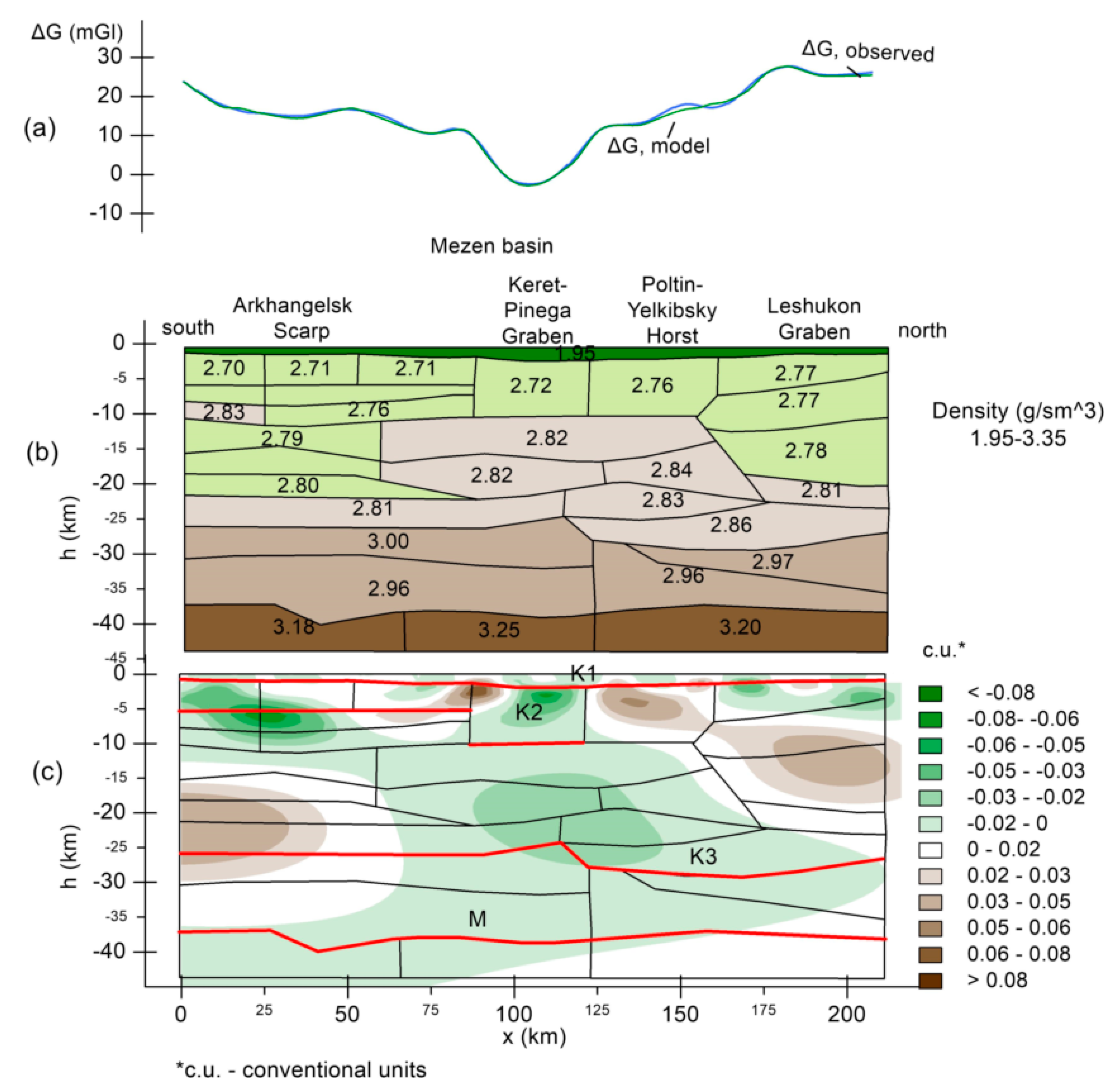
3.1. 2D Modelling Example

Figure 3 shows a 2D density model of a fragment of AGATE 3 geotraverse (Ust Pinega-White Sea), demonstrating the layered-block structure of the earth’s crust [18]. The fragment is oriented across the main deep faults at the contact of the eastern part of the Kola and Karelian geoblocks, and extends across the Arkhangelsk Scarp, the Keret-Pinega Graben, the Poltin-Yelkib Horst, and the Leshukov Graben from south to north. The trend of the gravity field and the density distribution of the rocks in the 2D model reflect the boundaries of these rock units. The profile clearly shows the boundaries of the basement (depth 1–4 km, V_p = 6.0–6.3 km/s) and M-discontinuity (depth 36–40 km, V_p = 8.0–8.2 km/s). Manifested in geophysical fields, heterogeneities refer to the upper and middle crust. The lower crust with P-wave velocity of 6.8–7.1 km/s has a nearly uniform distribution of petrophysical parameters.

The boundaries of the layers of the reference velocity model in Figure 3 are highlighted in red. Such boundaries for all considered profiles define the frame of the 3D surface of the layer.

3.2. 3D Density Model of the White Sea Region

Figure 4 shows a 3D density model of the White Sea region (a) and the position of the reference velocity model’s layer boundaries in space (b). To simplify the picture, the positions of the layer boundaries are shown as in-depth contours obtained by the Isolines procedure of Integro in Figure 5.

As the diagram of the K1 surface depth (Figure 5a) shows, the sedimentary layer is present in some parts of the region and is mainly traced in the directions of the inflow of sedimentary material by the Severnaya Dvina and Mezen rivers. There is no sedimentary layer in Onega and at part of the Kandalaksha bay, near the Tersk Shore of the White Sea. Its maximum thickness of 6 km is observed at the confluence of the river Mezen in the White Sea and the White Sea Funnel.

The bedrock surface of the “granite-metamorphic layer K1–K2” (Figure 5b) is lowered in the southwestern and northeastern directions, in the Keret, Padun, and Leshukon grabens. In the central part, the depression is confined to the sedimentation basins of the Severnaya Dvina and Mezen rivers. The “granulite-basic layer K2–K3” (Figure 5c) varies in thickness from near-zero values to 30 km. A large area is occupied by the southwestern depression of its lower boundary. The Zimny Bereg Uplift is represented by a zone of differently directed gradients on its lower surface, and the depression is outlined in the White Sea Throat, which contrasts more in the topology of the M-discontinuity (Figure 5d).

On the M-surface, the depression in the White Sea Throat is surrounded by uplifts near the Mezen, the Tersk Shore of the White Sea, and Kanin Nos Peninsula. The maxima of M-depression are consistent with positive Bouger anomalies and the minima with negative anomalies (Figure 2).

3.3. Alternative Map of the M-Border

To check the simulation results, an attempt to obtain some of them independently was made. It is most convenient to carry out such a check on the example of M-discontinuity. Due to the density jump, this boundary is confidently fixed on seismic profiles, and its features are manifested in the anomalous gravity field in the Bouger reduction, overlying layers of the earth’s crust and the relief of the earth’s surface [37]. A linear regression equation:

$$Z_M=39.54-0.0354\cdot \Delta G-0.0071\cdot h$$

(2)

is calculated by connecting the depth Z (km) of the M-discontinuity on available seismic profiles, the value of the anomalous gravity field in the Bouguer reduction ΔG (mGl), and the elevation of the relief h (m) (Figure 6a,b). Using Equation (2), an alternative map of the depth of the M-discontinuity surface was constructed and the result is shown in Figure 6c. The map, with smoothed local features, in general correctly reflects the general plan of the structure of the M-discontinuity shown in Figure 5d.

4. Discussion

The well-defined crustal structure of a 3D model of the region in the form of alternating variably deep layers with differences (Figure 4b) is consistent with generally accepted geological concepts.

The real structure of the earth’s crust is complex. Instrumental measurements indicate the existence of high-speed interlayers in low-density layers, as, for example, in Figure 3c, or asthenospheric lenses at the boundary of the earth’s crust and mantle. Nevertheless, the obtained 3D density structure of the earth’s crust can be used to describe the deep structure of the region, clarify the structural boundaries, and develop criteria for identifying promising areas for the search for minerals.

The absence of the sedimentary layer in a part of the White Sea (Figure 5a) may be caused by the uplift of these parts associated with the Fennoscandian shield. A thick sedimentary layer in the White Sea Funnel hinders deep water exchange in the White and Barents Seas and is one of the causes of the low salinity of the White Sea, about 26 ppm, and associated ecological and biological effects.

The uplifts of the underlying surface of the “granite-metamorphic layer” fall on the structures of the Karelian and Kola megablocks, the Zimny Bereg Uplift, and the Onega peninsula (Figure 5b). In this connection, the Zimny Bereg Uplift and the Onega Peninsula can be considered as the continuation of the structures of the Tersk coast of the White Sea and the Karelian megablock, respectively.

An example of the connection of the layer’s form with geological processes is provided by the depression of the M-discontinuity, identified in the White Sea Throat. The results of modelling generalized empirically show that there is a subvertical crustal structure near the Zimny and Tersk Shores, the White Sea Throat, and the White Sea Funnel associated with kimberlite magmatism. Diatremes, sills, and explosion pipes are located in some parts of the Archean-Early Proterozoic crust with a mosaic type of geophysical anomaly and are confined to linear tectonic zones [12].

The depression of the M-discontinuity in the White Sea Throat, reflecting earth crust–mantle interaction, is a criterion for diamond potential [38]. The similarity of its local extrema (Figure 5d) indicates the interpenetration, mixing, and transformation of deep-seated matter in the conjugation zone of the uplifting Fennoscandian Shield and the Russian Plate. Geodynamically, this process is contrary to tectonic plate subduction. The Zimny Bereg Diamondiferous Province is associated with an old crystalline basement scarp, which is constantly uplifting. The Zimny Bereg kimberlite field is located in a NW-trending Riphean aulacogen, in the Kola Craton-Mezen syneclise conjugation zone. The gravity field of the aulacogen passes from weakly negative to positive values. The magnetic field values are elevated. Gravity and magnetic anomalies in lower crustal layers, affected by low heat flow, indicate a deep source of magma generation. Regional faults and areas of intersection of tectonic zones display deformations, fastenings, the steep bends of the contour lines of gravity and magnetic fields, and the geochemical aureoles of Ni, Mn, Cr, Co, and Zn. Ultramafic explosion pipes, occurring in the crystalline basement with high electrical resistance, exhibit elevated conductivity [12,19].

5. Conclusions

Two- and three-dimensional density models of the White Sea region’s crust were developed based on the results of well-known seismic and gravimetric instrumental studies using the Integro software complex. In the 3D density model, the positions of the boundaries of the speed layers of the earth’s crust of the region were determined.

Boundary surface relief schemes allow the local features of layer’s boundaries to be geographically referenced, features to be associated with gravitational field anomalies, and the power of Earth’s crust layers to be estimated.

The proposed interpretation of the simulation results explains the absence of a sedimentary cover on part of the water area and its large capacities in the deep-sea areas by raising of the Fennoscandian shield. Connections within the framework of the granite-metamorphic layer of the Winter Bank Uplift and the Onega Peninsula with the structures of the Terek Coast and the Karelian Megablock, respectively, are indicated, in addition to large capacities of the granulite-basite layer in the area of Winter Bank lifting by the intensity of its formation, and the depression of the M boundary by the existence of a subvertical structure associated with manifestations of kimberlite magmatism.

References

1. Baluev, A.S.; Brusilovskii, Y.V.; Ivanenko, A.N. The crustal structure of Onega-Kandalaksha paleorift identified by complex analysis of the anomalous magnetic field of the White Sea. Geodyn. Tectonophys. 2018, 9, 1293–1312. [Google Scholar] [CrossRef]
2. Konstantinovsky, A.A. Rifeisky Onega-Kandalakshsky graben of the East European Platform. Geotectonics 1977, 3, 38–45. (In Russian) [Google Scholar]
3. Dobrynina, M.I. Riftogenesis in the Geological History of the Precambrian of the Northern part of the Russian Plate. Deep Structure and Geodynamics of Crystal Shields of the European Part of the USSR; Mitrofanov, F.P., Bolotov, V.I., Eds.; Publishing House of the KSC RAS: Apatites, Russia, 1992; pp. 71–78. (In Russian) [Google Scholar]
4. Sim, L.A.; Postnikov, A.V.; Postnikova, O.A.; Poshibaev, V.V. Influence of the latest geodynamics on the gas content of the Irkineyevo-Chadobetsky riftogenic deflection. Expo. Oil Gas 2016, 6, 8–12. (In Russian) [Google Scholar]
5. Kazanin, G.S.; Zhuravlev, V.A.; Pavlov, S.P. The structure of the sedimentary cover and the White Sea’s oil and gas potential. Buren. Neft. 2006, 2, 26–28. (In Russian) [Google Scholar]
6. Kheraskova, T.N.; Sapozhnikov, R.B.; Volozh, Y.A.; Antipov, M.P. Late Precambrian geodynamics and evolution of the northern East European Platform, as shown by regional seismic profiling. Geotektonika 2006, 6, 33–51. (In Russian) [Google Scholar]
7. Aplonov, S.V.; Fedorov, D.L. (Eds.) Geodynamics and Oil and Gas Potential of the Mezen Sedimentary Basin; Nauka: Sant Petersburg, Russia, 2006; 319p. (In Russian) [Google Scholar]
8. Zhuravlev, V.A. Earth crust structure of the White Sea Region. Razved. i Okhrana Nedr. 2007, 9, 22–26. (In Russian) [Google Scholar]
9. Zhuravlev, V.A.; Shipilov, E.V. Structure of basins in the White Sea rift system. Okeanologia 2008, 48, 123–131. (In Russian) [Google Scholar] [CrossRef]
10. Baluev, A.S.; Zhuravlev, V.A.; Terekhov, A.N.; Przhiyalgovsky, E.S. Tectonics of the White Sea and Adjacent Areas (Explanatory Note to a “1: 500 000 Tectonic Map of the White Sea and Adjacent Areas” 1:500000); GEOS: Moscaw, Russia, 2012; 104p. (In Russian) [Google Scholar]
11. The White Sea System. Sedimentation, Geology and History; Nauch. Mir: Moscaw, Russia, 2017; Volume 4, 1030p. (In Russian)
12. Kutinov, Y.G.; Chistova, Z.B.; Polyakova, E.V.; Mineyev, A.L. Digital modelling of relief for forecasting of areas with oil and diamonds. Acute Oil Gas Probl. 2019, 24. (In Russian) [Google Scholar] [CrossRef] [Green Version]
13. Sharov, N.V.; Mitrofanov, F.P.; Verba, M.L.; Gillen, C. (Eds.) Lithospheric structure of the Russian Barents Sea Region; KarRC. RAS: Petrozavodsk, Russia, 2005; 318p. (In Russian) [Google Scholar]
14. Sharov, N.V.; Slabunov, A.I.; Isanina, E.V.; Krupnova, N.A.; Roslov, Y.V.; Shchiptsova, N.I. Seismic section of the earth crust along the DSS-CDP profile «Land-Sea» Kalevala-Kem-White Sea Throat. Geofiz. Zhurn. 2010, 32, 21–34. (In Russian) [Google Scholar]
15. Glaznev, V.N.; Raevsky, A.B.; Skopenko, G.B. A three-dimensional integrated density and thermal model of the Fennoscandian lithosphere. Tectonophysics 1996, 258, 15–33. [Google Scholar] [CrossRef]
16. Glaznev, V.N.; Mints, M.V.; Muravina, O.M.; Raevsky, A.B.; Osipenko, L.G. Complex geological—Geophysical 3D model of the crust in the southeastern Fennoscandian sheild: Nature of density layering of the crust and the crust—Mantle boundary. Geodyn. Tectonophys. 2015, 6, 133–170. [Google Scholar] [CrossRef] [Green Version]
17. Konanova, H.B. Volumetric models of the gravimetric field of the Timan-North Uralian Region and adjacent areas. Bull. Inst. Geol. Komi Sci. Cent. Ural Branch Russ. Acad. Sci. 2010, 9, 8–14. (In Russian) [Google Scholar]
18. Mints, M.; Suleimanov, A.; Zamozhniaya, N.; Stupak, V. A 3-D model of the Early Precambrian crust under the south-eastern Fennoscandian Shield: Karelia Craton and Belomorian tectonic province. Tectonophysics 2009, 472, 323–339. [Google Scholar] [CrossRef]
19. Pospeyeva, E.V.; Vitte, L.V. Structural characteristics of the earth crust of the White Sea block and part of the Karelian block, as shown by magnetotelluric studies. Geofizika 2011, 3, 64–72. (In Russian) [Google Scholar]
20. Cheremisina, E.N.; Finkelstein, M.Y.; Lyubimova, A.V. GIS INTEGRO—An import-replacing software-technological complex for solving geologo-geophysical problems. Geoinformatika 2018, 3, 8–17. (In Russian) [Google Scholar]
21. Sharov, N.V.; Zhuravlev, A.V. Crustal structure of the White Sea and adjacent areas. Arct. Ecol. Econ. 2019, 3, 62–72. (In Russian) [Google Scholar] [CrossRef]
22. Sharov, N.V.; Bakunovich, L.I.; Belashev, B.Z.; Zhuravelev, A.V.; Nilov, M.Y. Geologo-geophysical models of the earth crust of the White Sea Region. Geodyn. Tectonophys. 2020, 11, 566–582. (In Russian) [Google Scholar] [CrossRef]
23. Mitrofanov, F.P.; Sharov, N.V.; Zagorodny, V.G.; Glaznev, V.N.; Korja, A.K. Crustal Structure of the Baltic Shield along the Pechenga-Kostomuksha-Lovisa Geotraverse. Intern. Geol. Rev. 1998, 40, 990–997. [Google Scholar] [CrossRef]
24. Sharov, N.V. Lithosphere of Northern Europe, as Shown by Seismic Data; KarRC RAS: Petrozavodsk, Russia, 2017; 173p. (In Russian) [Google Scholar]
25. Pimanova, N.N.; Spiridonov, V.A.; Sharov, N.V.; Lyubimova, A.V.; Senner, A.E. Distribution of density heterogeneities in the earth crust and mantle of the southeastern Fennoscandian Shield, as shown by geological and geophysical data. Geoinformatika 2018, 1, 43–51. (In Russian) [Google Scholar]
26. Sapozhnikov, R.B. Efficiency of EWM DP seismic prospecting for the study of the geological structure of the Mezen syneclise. Razved. Okhrana Nedr. 2003, 5, 32–35. (In Russian) [Google Scholar]
27. 1:1000000 Scale State Geological Map of the Russian Federation (Third Generation). Baltic Series. Sheet Q-(35), 36—Apatity. Explanatory Note; VSEGEI Cartographic Factory: Murmansk/Sant Peterburg, Russia, 2009; 487p. (In Russian)
28. 1:1000000 Scale State Geological Map of the Russian Federation (Third Generation). Baltic Series. Sheet Q-37- Arkhangelsk. Explanatory Note; VSEGEI Cartographic Factory: Murmansk/Sant Peterburg, Russia, 2009; 338p. (In Russian)
29. 1:1000000 State Geological Map of the Russian Federation (Third Generation). Mezen Series. Sheet Q-38- Mezen. Explanatory Note; VSEGEI Cartographic Factory: Murmansk/Sant Peterburg, Russia, 2009; 350p. (In Russian)
30. Sharov, N.V. (Ed.) Deep Structure and Seismicity of the Karelian Region and Surrounding Areas; KarRC RAS: Petrozavodsk, Russia, 2004; 353p. (In Russian) [Google Scholar]
31. Erinchek, Y.M. (Ed.) A Model of the Earth Crust and the Upper Mantle Based on Deep Seismic Profiling; VSEGEI: Sant Peterburg, Russia, 2007; 245p. (In Russian) [Google Scholar]
32. Pimanova, N.N.; Biserkin, I.A.; Deev, K.V. Technology for constructing 3D density models in the Integro GIS environment. Geoinformatics 2013, 4, 45–48. (In Russian) [Google Scholar]
33. Kobrunov, A.I. Mathematical Foundations of the Theory of Interpretation of Geophysical Data; TsentrLitNefteGaz: Moscow, Russia, 2008; 286p. (In Russian) [Google Scholar]
34. Priezzhev, I.I. Construction of distributions of physical parameters of the environment according to the data of gravity prospecting, magnetometry. Geophysics 2005, 3, 46–51. (In Russian) [Google Scholar]
35. Mitsyn, S.V.; Ososkov, G.A. Extrapolation of grid models of geophysical fields by the finite difference method. Geoinformatics 2016, 3, 29–34. (In Russian) [Google Scholar]
36. Deev, K.V. Multilevel two-dimensional interpolation in the processing of geological and geophysical information. Geoinformatics 2003, 2, 55–59. (In Russian) [Google Scholar]
37. Kashubin, S.N.; Petrov, O.V.; Androsov, E.A.; Morozov, A.F.; Kaminsky, V.D.; Poselov, V.A. A map of the crustal thickness of Circumpolar Arctic. Reg. Geol. Metallog. 2011, 46, 5–13. (In Russian) [Google Scholar]
38. Golubev, Y.K.; Vaganov, V.I.; Prusakova, N.A. Principles of forecasting diamondiferous areas on the East European Platform. Rudy Met. 2005, 1, 55–70. (In Russian) [Google Scholar]
Figure 1. Main structural elements of the White Sea region.
Geosciences 10 00492 g001
Figure 2. The layout of seismic profiles and the regional component of the gravity field in the Bouger reduction in the White Sea and adjacent territories.
Geosciences 10 00492 g002
Figure 3. 2D density model for a section of the seismic profile AGATE 3 (Ust Pinega-White Sea): graphs of observed profile Bouger anomaly and model calculated field (a), density block model based on seismic data (b), and distribution of effective density with boundaries of velocity layers determined from seismic data shown in red (c). Conventional units characterize effective density distribution as normalized deviations. The pattern of seals and decompressions in the profile of the earth’s crust (c) is given by the results of the Integro procedure of the section 3D density model by 2D profile [20,25].
Geosciences 10 00492 g003
Figure 4. Three-dimensional model of the density distribution of the earth’s crust of the White Sea region (a) and spatial representation of the boundary surfaces K1, K2, K3, and M of the velocity layers of the region’s earth crust (b).
Geosciences 10 00492 g004
Figure 5. Schemes of the depths of the surfaces K1 (a), K2 (b), K3 (c), and M (d).
Geosciences 10 00492 g005
Figure 6. Regression model in the deep seismic sections relating the depth of occurrence of M-discontinuity (Z, km) to Bouger anomaly (ΔG, mGl) and the topographic mark (h, m). (a) Reference data related to land and sea are shown in pink and sky-blue, respectively, and model results in blue; (b) position of the regression plane of the M-discontinuity in the coordinate system a; (c) map of the depths of occurrence of M-discontinuity based on Equation (2) and combined with data on deep seismic sounding (DSS) profiles.
Geosciences 10 00492 g006