The Effect of Targeted Field Investigation on the Reliability of Earth-Retaining Structures in Passive State: A Random Field Approach

Abstract

In one of their recent works, the authors examined parametrically the effect of targeted field investigation on reducing statistical uncertainty in active state analysis of earth retaining structures based on 2165 different cases for each of the sliding and overturning modes of failure. This analysis indicates that the optimal sampling location is always adjacent to the wall, while a sampling domain length equal to the whole height of the wall is suggested to be considered. The present paper deals with the “symmetrical” problem of soil under the passive state of stresses. Working in a similar manner, 1879 passive state cases have been considered (also for each of the sliding and overturning modes of failure) in a Random Finite Element Method (RFEM) analysis framework, where soil properties are modeled as random fields while measurements are modeled by sampling from different points of the field domain. The “actual” resultant earth passive pressure force (or moment) exerted by the random soil on the retaining wall is compared against the respective “predicted” one calculated using the soil property values sampled from the random field. Failure is considered to have occurred when the derived “actual” force is smaller than the respective “predicted” force. This analysis clearly indicates that the passive state constitutes a different problem, where the optimal sampling distance from the wall is half the wall height. Regarding the depth of exploration, it was again found to be the entire wall height. In addition, the present analysis shows that, the benefit from a targeted field investigation is much greater than the benefit gained using statistical methods for obtaining cautious estimates for the various soil properties; the latter refers to the “characteristic value”, a concept commonly used in the Limit State analysis framework of Eurocode 7.

1. Introduction

The inherent variability, systematic uncertainty and statistical uncertainty are the three main sources of uncertainty regarding soil property values [1]. The inherent variability refers to the variability that the soil properties exhibit by nature, even in seemingly homogenous soil media. Discrepancies between in situ conditions and laboratory are related to systematic uncertainties [1,2,3]. Statistical uncertainty is related to limited soil testing, i.e., to the fact that the soil mass, which is affected, is much greater in volume than the soil mass tested in the field or in the lab. Regarding statistical uncertainty, it is worth mentioning that current design codes (e.g., AASHTO [4] or EN 1997-2:2007 [5]) give some general recommendations (see also Appendix A in [6]) related to the extent of the subsurface exploration and aiming at identifying possible unfavorable geological conditions.

The effect of soil sampling on the performance of geotechnical structures has been investigated, so far, by the following researchers. Ching and Phoon [7] attempted to fully characterize the statistical uncertainty in the unknown trend function for the vertical spatial distribution of geotechnical site investigation data. Fenton et al. [8] studied the effect of the type of trend removal and the number of samples on residual uncertainty. Yang et al. [9,10] and Li et al. [11] studied the importance of soil property sampling location in slope stability analysis. Jaksa et al. [12] and Christodoulou and Pantelidis [13], on the other hand, studied the importance of soil property sampling location in footing’s settlement analysis. Griffiths et al. [14] studied the effect of sampling on the reliability of earth pressure analysis in the passive state based on the Random Finite Element Method (RFEM). Based on four sampling locations, they drew the conclusion that a single sampling point located at an offset distance equal to approximately one wall height from the wall results to lower probability of failure and that this probability is reduced when additional sampling points are considered. Finally, in one of their recent works, the authors [6] examined the effect of targeted field investigation on reducing statistical uncertainty in active state analysis of earth retaining structures. The parametric analysis in question, involving 2165 different cases for each of the sliding and overturning modes of failure, indicates that the optimal sampling location is at zero distance from the wall, while the sampling domain length should preferably be equal to the wall height. The present paper deals with the effect of targeted field investigation on the reliability of earth retaining structures in passive state. This is done through an extensive parametric analysis (1879 passive state cases have been considered in total for each of the sliding and overturning modes of failure) using the RFEM method [15], properly considering soil sampling in the analysis. Apparently, the present analysis refers to, e.g., sheet pile and bored pile walls, retaining undisturbed soil (otherwise sampling makes no sense).

2. Parametric Analysis for Determining the Optimal Sampling Strategy

This paper examines in a RFEM framework the case of a wall retaining fully drained cohesionless soil against passive failure. The REARTH2D program (freely available at http://www.engmath.dal.ca/rfem) is used. As mentioned below, the program in question has been modified by the authors to accommodate the needs of the present research. The REARTH2D program generates and maps onto a finite element mesh the various spatially random soil properties (e.g., the friction angle); each one of these random fields is fully described by its mean, standard deviation and scale of fluctuation. For a specific set of material random fields, the program calculates both the wall reaction force and overturning moment caused by the self-weight of soil (these are called “actual” forces and moments). It also calculates the respective (“predicted”) force and moment based on Rankine’s [16] theory for earth pressures using the mean of the values sampled from each soil property field. m realizations are considered, where in each of these realizations a new set of random fields for c′, ϕ′, and γ is generated. The “probability of failure” (p_f) of the retaining wall is then calculated both for the sliding and the overturning mode of failure; p_f is defined by the fraction of the number of realizations that result in a sliding or overturning failure over the total number of realizations. “Failure” is considered to have occurred when the “actual” wall reaction force or overturning moment (value calculated using the RFEM method i.e., considering that the soil is spatially random) is smaller than the respective (factored or unfactored) predicted value referring to soil having spatially uniform properties sampled from the RFEM random fields:

$$p_f=P\left[X_{p,RFEM}<\frac{X_{p,Rankine}}{FS}\right] \mathrm{or} P\left[X_{p,“actual”}<\frac{X_{p,predicted}}{FS}\right]$$

(1)

where the symbol X denotes either the wall reaction force or the overturning moment (F and M respectively). FS is the factor of safety considered in the analysis or, in Eurocode 7 [17] terms, the model factor.

The REARTH2D program was modified by the authors so as the “predicted” magnitudes to be calculated using the finite element method (and not Rankine’s theory), while the mean of the values sampled from each soil property field is also used. That is,

$$p_f=P\left[X_{p,RFEM}<\frac{X_{p,FEM}}{FS}\right] \mathrm{or} P\left[X_{p,“actual”}<\frac{X_{p,predicted}}{FS}\right]$$

(2)

In the RFEM analysis below, the soil mass is discretized into a 60 by 34 mesh of eight-noded quadrilateral elements (in the horizontal and vertical direction respectively); the length of the edge of each element is equal to 0.1m (see Figure 1). A 24-element wall is extensively used below, which hereafter is called the “reference wall”. For investigating the effect of wall height on the optimal sampling strategy, wall heights ranging from H = 1.4 m to 2.9 m (i.e., 14 to 29 elements respectively) were considered. The 60 elements in the horizontal direction were chosen so that any undesirable boundary effect to be eliminated.

Ε and ν was found not to have any influence on the optimal sampling strategy, thus, all figures given below stand for any Ε and ν pair of values. Therefore, in the present analysis only ϕ′ and γ are treated as random fields with μ_ϕ′ = 30°, μ_γ = 20 kN/m³ and COV of ϕ′ and γ equal to 0.3. Throughout the entire analysis, the values of ν and Ε were held spatially constant at ν = 0.3 and Ε = 10⁵ kN/m², while various standard deviation and scale of fluctuation values of soil strength are examined. It is noted that the soil considered is cohesionless, whilst both ϕ′ and γ are assumed to be log-normally distributed [15,18,19,20,21]. K_o, for establishing the initial state of stresses, is also treated as random field as being a pure function of ϕ′ (according to Jaky [22] K_o = 1 − sinϕ′). Finally, a factor of safety FS equal to 1.25 is generally used in the analysis, although the effect of FS on the sampling strategy is also subject matter of the present paper.

In the parametric analysis below both the sampling from a single point and sampling from domain strategies are examined. Aiming at finding the sampling strategy that minimizes the statistical error (called optimal sampling strategy), the following parameters are examined: the sampling depth (d_p) or the sampling domain length (d_d) for the case of sampling from a single point and the case of sampling from a domain, respectively (both measured from the soil surface; the latter rather refers to continuous probing test data), the horizontal sampling distance (x) measured from the wall face, the scale of fluctuation of soil (θ), the wall roughness (the wall is considered either perfectly smooth or perfectly rough), the height of the wall (H), the COV and mean value of ϕ′, the factor of safety value (FS), and the anisotropy of soil mass (θ_h ≠ θ_v). The symbol θ (that is, without subscript) denotes, hereafter, isotropic conditions (θ_h = θ_v). The reduction of statistical error is quantified through the reduction in p_f when adopting different sampling scenario. Figure 2 illustrates examples of different sampling scenarios, referring either to a single point (scenarios A and B) or to continuous probing tests (scenarios C and D).

The optimal sampling point or domain will be identified by comparing the probability of failure (p_f) values derived by various sampling strategies. Because the present analysis deals with small differences in p_f values, the number of realizations was set to 3000 for obtaining stable results (see Appendix A in the present paper). The element size was chosen to be half of the smallest scale of fluctuation considered in this study (see [6,23]).

2.1. Sampling from a Single Point

2.1.1. Effect of Scale of Fluctuation (θ)

A number of p_f − d_p/H example curves have been drawn in Figure 3 for various θ/H and x/H values both for the case of sliding and overturning mode of failure. From this figure, it is clear that the optimal sampling distance from the wall in the passive state is 0.5H from the wall face, both for sliding and overturning modes of failure; this stands for any θ value. It is also interesting that, there is a worst case θ/H value, where p_f becomes maximum (see Figure 4). From Figure 4, it is also inferred that when θ is very small, p_f does not depend on the sampling depth. However, p_f value becomes more dependent on the sampling depth as θ increases.

2.1.2. Effect of Wall Roughness

Comparing Figure 5 (perfectly rough wall) with Figure 4 (perfectly smooth wall) it is inferred that the roughness of the wall has minor effect on the optimal sampling depth, in a manner that, in smooth walls, the optimal sampling point appears to be slightly higher. In addition, it is observed that the optimal sampling point appears to be higher for the overturning mode of failure (the same happens in the case of smooth walls). Because the wall roughness was found by the authors not to affect the optimal sampling distance, where again the half wall height (x/H = 0.5) is the best choice for conducting field investigation, thus, curves were drawn only for this sampling distance (see Figure 5).

2.1.3. Effect of Wall Height

In this respect, different wall heights, ranging from 1.4 to 2.9m with 0.5m interval, were considered. From the p_f − d_p/H curves of Figure 6, it is obvious that, the wall height has only a minor influence on the location of the optimal sampling point, mainly in the case only of the sliding wall.

2.1.4. Effect of COV of ϕ′

In this respect, it was found that the optimal sampling distance from the wall face is not affected by the COV of ϕ′, where, again, a distance equal to a half wall height leads to smaller statistical error; five different COV values of ϕ′ have been considered, ranging from 0.1 to 0.5, with 0.1 interval. Thus, only the x/H = 0.5 case is presented here. From Figure 7, it is concluded that the COV of ϕ′ has no influence on the optimal sampling depth; the same stands both for the case of sliding and overturning wall.

2.1.5. Effect of μ_ϕ′ value

Three different μ_ϕ′ values (μ_ϕ′ = 20, 30, and 40°) were considered here for examining the effect of the mean value of ϕ′ to the sampling strategy (the COV of ϕ′ and γ were equal to 0.3 and 0, respectively). The analysis showed that the optimal horizontal sampling distance is for x/H = 0.5 and it is independent of the μ_ϕ′ value. Moreover, as shown in Figure 8, the optimal sampling depth is also independent of μ_ϕ′ (something that stands both for the case of sliding and overturning modes of failure).

2.1.6. Effect of the Factor of Safety (FS)

The optimal sampling distance from the wall face was found at x/H = 0.5 for any FS value; thus, p_f − d_p/H curves are given only for this value (see Figure 9). As expected, p_f decreases as FS increases. However, it is interesting that the positive effect of a targeted field investigation on the reduction of the statistical error is greater for greater FS values.

2.1.7. Effect of Soil Anisotropy

Generally, soils appear to be more variable in the vertical direction than in the horizontal direction and this is attributed to the natural deposition and the soil formation processes. Roughly, the scale of fluctuation of soil in the vertical direction is 10 times smaller than the respective scale of fluctuation in the horizontal direction [24,25,26,27,28]. Considering this, the effect of soil anisotropy on the optimal sampling location is investigated herein comparing the θ_v/H = θ_h/H = 2.08 case with the θ_v/H = 2.08 and θ_h/H = 20.8 case. The “reference” wall-soil system is used, whilst the results are presented in Figure 10 in the usual p_f versus d_p/H form for various x/H values. From this figure, it is concluded that the horizontal distance plays, generally, no role in the statistical uncertainty, especially when x/H < 1. In addition, soil anisotropy seems not to affect the depth of the optimal sampling location, either in the case of the sliding or overturning wall. However, anisotropic soils rather give smaller p_f values (please compare Figure 10a,b with Figure 3c,d, respectively).

2.2. Sampling from a Domain

The “sampling from a domain” strategy may refer to continuous undisturbed sampling in the field (followed by suitable laboratory tests for obtaining the required soil parameters) or to continuous probing test data, such as those obtained from, e.g., the Cone Penetration Test or Standard Penetration Test. In the analysis below, the length of the sampling domain is measured from the soil surface. Virtual sampling is considered to take place with 0.1 length unit interval (in this respect, meters), as each (square) element in the finite element mesh used has this edge length. The arithmetic mean of the values sampled from each soil property random field is used in the finite element analysis (recall Equation (2)). It is noted that, for all cases examined in this section, the x/H = 0.5 distance from the wall was again found to be optimal. Thus, for keeping the length of the present paper in a logical length, only this case is presented below.

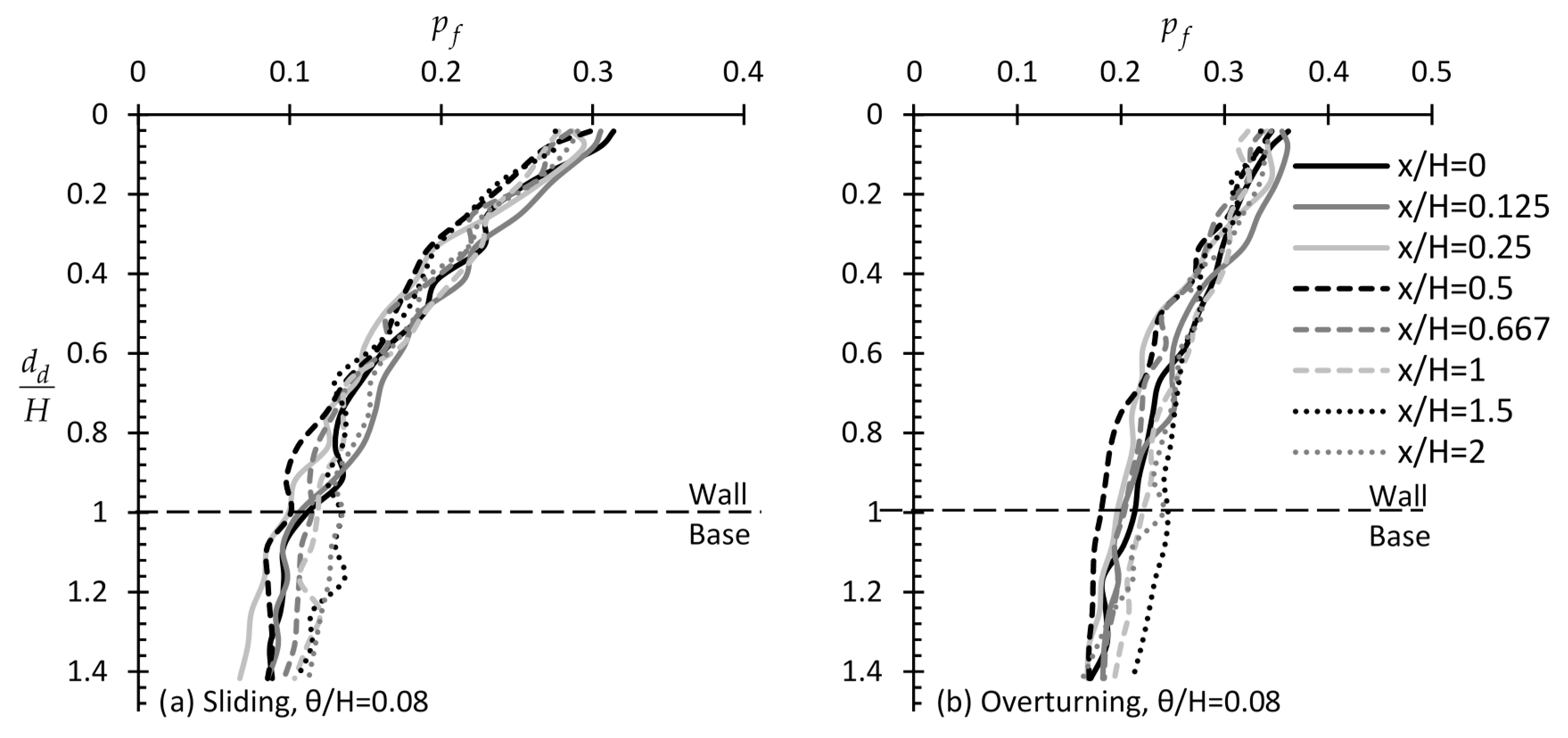
2.2.1. Effect of Scale of fluctuation (θ)

From the p_f versus d_d/H charts of Figure 11 it is clear that the optimal horizontal sampling distance from the wall is again for x/H = 0.5. Indeed, when θ is very small, a different sampling distance seems not to greatly affect the statistical error. On the contrary, as θ increases the role of horizontal distance becomes more and more significant. In the figure in question, x/H values ranging from 0 to 2 were considered, whilst FS was set equal to 1.25 (recall Equation (2)). Furthermore, it is suggested that the entire domain length at horizontal distance equal to half wall height from the wall be considered for reducing the statistical error to a minimum possible level. It is also worth noting that if the sampling domain length is extended below the lower point of the wall (i.e., d_d/H > 1), the statistical error is not greatly affected (the present analysis considered normalized depths d_d/H up to 1.4). Finally, as shown in Figure 12 (also observed in Figure 11), there is a worst-case theta (value giving greater p_f values as compared to the other θ values).

2.2.2. Effect of Wall Roughness

As expected, the wall roughness affects the probability of failure however it has minor influence on the optimal sampling domain length, where the entire wall height is suggested to be taken into account (see Figure 13). Even greater sampling domain lengths have no influence in the reduction of the statistical error.

2.2.3. Effect of Wall Height

In this respect, four wall heights ranging from 1.4 to 2.9 m with 0.5 m interval, were considered. From the p_f − d_d/H curves of Figure 14, it is clear that the wall height largely affects the statistical error with the higher walls requiring greater sampling domain length, especially in the case of the sliding wall. For both sliding and overturning walls, it is advisable that the whole domain length be taken into account.

2.2.4. Effect of COV of ϕ′

As shown in Figure 15, the COV of ϕ′ has no influence on the sampling strategy, where again the half wall height is the optimal sampling distance from the wall, whilst it is advisable that a domain length equal to the wall height be considered. Five different COV values of ϕ′ were considered, ranging from 0.1 to 0.5 with 0.1 interval. For the economy of space, only the x/H = 0.5 case is presented herein.

2.2.5. Effect of the Factor of Safety (FS)

The analysis on the effect of FS on the sampling strategy did not reveal anything different from what has been reported above, where the optimal sampling strategy refers to x/H = 0.5 and d_d/H = 1. As expected, p_f decreases as FS increases, however, the FS value has no influence on the optimal sampling domain length (see Figure 16).

2.2.6. Effect of Soil Anisotropy

The anisotropic case was examined considering θ_h/H = 20.8 and θ_v/H = 2.08 (it is reminded that the isotropic case has θ_h/H = θ_v/H = θ/H = 2.08; see Figure 11). As it is inferred from Figure 17, the soil anisotropy has minor effect both on the probability of failure and the optimal sampling domain length. For both cases (the sliding and overturning wall) the statistical error remains relatively constant for horizontal sampling distances less than the wall height. By taking samples in distance greater than that, the statistical error increases slightly.

3. Discussion

3.1. Optimal Sampling Locations

From the above extended parametric analysis, it is concluded that the optimal offset distance from the wall face for fully drained cohesionless soils is at half wall height, whilst the optimal sampling depth (referring to a single sampling point) is greater than the 2/3 and 1/2 of the height of the wall for the sliding and overturning modes of failure, respectively (the exact depth depends on the special variability of soil, i.e., the scale of fluctuation value). When a sampling domain is considered, the authors suggest that a length equal to the whole height of the wall be considered.

3.2. The Importance of Targeted Field Investigation in Practice

The importance of the findings is illustrated through the examples given below. Three specific random fields are considered, assuming that these represent in practice actual soil fields. These random fields of ϕ′ are shown in Figure 1, Figure 18 and Figure 19 whilst their characteristics are given in

Table 1. Summary of the soils’ characteristics used in the three examples (wall height H = 2.4 m).

Example	Random Field (s)	Distribution	μϕ′	μγ	COV	θ/H	Figure 1)
#1	ϕ′, γ	Log-normal	30°	20 kN/m3	0.3	8.3	1
#2	ϕ′	Log-normal	30°	20 kN/m3	0.3	4.2	18
#3	ϕ′	Log-normal	30°	20 kN/m3	0.3	0.42	19

¹⁾ Figures showing the random fields of ϕ′.

. The soils are cohesionless and fully drained. The reference wall and a factor of safety equal to unity are used in all three examples (the value of FS is a matter of discussion in the next paragraph). Because the mean and the COV value of the soil parameters does not affect the decision upon the sampling strategy, these values where kept the same for all examples.

For all three cases the predicted magnitudes (F and M) are compared against the actual ones using the ratios F_predicted/F_”actual” and M_predicted/M_”actual”. The results are summarized in the charts of Figure 20, Figure 21 and Figure 22; F_predicted/F_”actual” and M_predicted/M_”actual” values are given for various x/H and d_d/H values. The relative difference R_d defined as F_predicted/F_”actual” − 1 and M_predicted/M_”actual” − 1 is also given in each chart (see secondary vertical axis).

As shown in Figure 20, Figure 21 and Figure 22, both F_predicted/F_”actual” and M_predicted/M_”actual” ratios are unity or very close to unity for x/H = 0.5 and d_d/H = 1, this is indicative of the success of the present analysis. It should be noted that, any F_predicted/F_”actual” or M_predicted/M_”actual” value close or equal to unity for other x/H values does not necessarily indicate optimal sampling location; this can also happen coincidentally as the soil is random and may exhibit similar properties in other locations. From the same figures it is also clear that, the increasing number of samples is not a precondition for reducing statistical uncertainty; indeed, the opposite may occur (please compare the p_f ≈ 0.015 value in Figure 3e for x/H = 0.5 and d_p/H = 0.7 with the p_f ≈ 0.18 value in Figure 11e for x/H = 2 and d_d/H = 1 referring to a single and 24 sampling points respectively). Such examples can also be found in the present section; please compare the {x/H = 2.5, d_d/H = 1} case with the {x/H = 0.5, d_d/H = 0.25} case shown in Figure 22b, giving R_d,M ≈ 0.52 and −0.04, respectively.

3.3. Designing with Load and Resistance Factor Design (LRFD) Codes

Eurocode 7 [17] aims to achieve geotechnical designs with an appropriate target reliability by applying partial factors to characteristic values of geotechnical parameters. Model uncertainties and dimensional variations are absorbed by applying “partial factors” to actions, material properties, and/or resistances [29]. While Eurocode 7 uses characteristic values (cautious estimate of the mean of a set of values) so as to take account of the inherent variability of the soil, the various North America codes [4,30,31,32] use mean values for soil properties. The following statistical equation using 95% confidence level is often adopted in practice for the calculation of the characteristic value [6,13,29,33]:

$$X_k=X_m-\frac{t_{a;v_s}\cdot S_d}{\sqrt{n}}$$

(3)

The design value of a geotechnical parameter (X_d) derives from the respective characteristic value, using the following equation [17]:

$$X_d=X_k/{\gamma }_{{\rm M}}$$

(4)

(all parameters in Equations (3) and (4) are defined in the notation list).

For discussing the effectiveness of the characteristic and mean value concept in reliability of retaining structures under the passive state, two example charts were produced, referring to case #3 presented above; see Figure 23. In this figure the d_d/H = 1 case can be directly compared with the respective d_d/H = 0.25 case.

From Figure 23, it is clear that, despite the conservatism of the characteristic values, the characteristic value concept alone cannot effectively deal with the inherent variability of soils, and, thus, it cannot guaranty a conservative enough engineering study (let alone the use of mean soil property values). From the same figure, it is also clear that the benefit from a targeted field investigation is much greater as compared to the benefit gained using characteristic values. It is even more interesting that a factor of safety as high as 1.25 (recall Equation (2); model factor for Eurocode 7) does not necessarily guarantee a safe design. Such a factor simply displaces downwards (that is, to the safe side) the F_predicted/F_”actual” (or M_predicted/M_”actual”) versus x/H curves and as characteristically shown, its precise value needs special consideration.

The inclusion of the “characteristic value” concept in the REARTH2D code was done by the authors.

4. Conclusions

The statistical uncertainty related to the soil property values in an earth-retaining project may be significant, and, consequently, the probability of failure may also be very high. In the present paper the case of a wall retaining a fully drained cohesionless soil against passive failure is examined, indicating that the uncertainty in question can effectively be minimized only when targeted field investigation is performed, that is when the number and the location of the sampling points are carefully selected. And this because as samples are taken from a material field (i.e., the ground), which simultaneously is a stress field (stresses caused by the self-weight of the soil and any external load), the location of the optimal sampling points is affected by the coexistence of these two fields.

From the above extended parametric analysis, it is concluded that the optimal offset distance from the wall face for cohesionless, fully drained soils is half wall height, whilst the optimal sampling depth (referring to a single sampling point) is greater than the 2/3 and 1/2 of the height of the wall for the sliding and overturning modes of failure, respectively (the exact depth depends on the special variability of soil, i.e., the scale of fluctuation value). When a sampling domain is considered, the authors suggest that a length equal to the whole height of the wall be considered. It is reminded that the same sampling domain length was found for walls being in the active state; however, the optimal sampling distance in the state in question is 0, i.e., in contact with the wall (please see the companion paper [6] published by the authors).

In addition, it is concluded that, despite the use of conservative soil property values (use of characteristic values), the characteristic value concept alone cannot effectively deal with the inherent variability of soils and, thus, it cannot guaranty a conservative enough engineering study. Indeed, the benefit gained from a targeted field investigation is much greater as compared to the benefit gained using characteristic values. Finally, the use of the model factor in a Load and Resistance Factor Design (LRFD) also needs special consideration as, depending on the soil variability, it does not necessarily guarantee a safe design.