The Effect of Targeted Field Investigation on the Reliability of Axially Loaded Piles: A Random Field Approach


Abstract
:1. Introduction
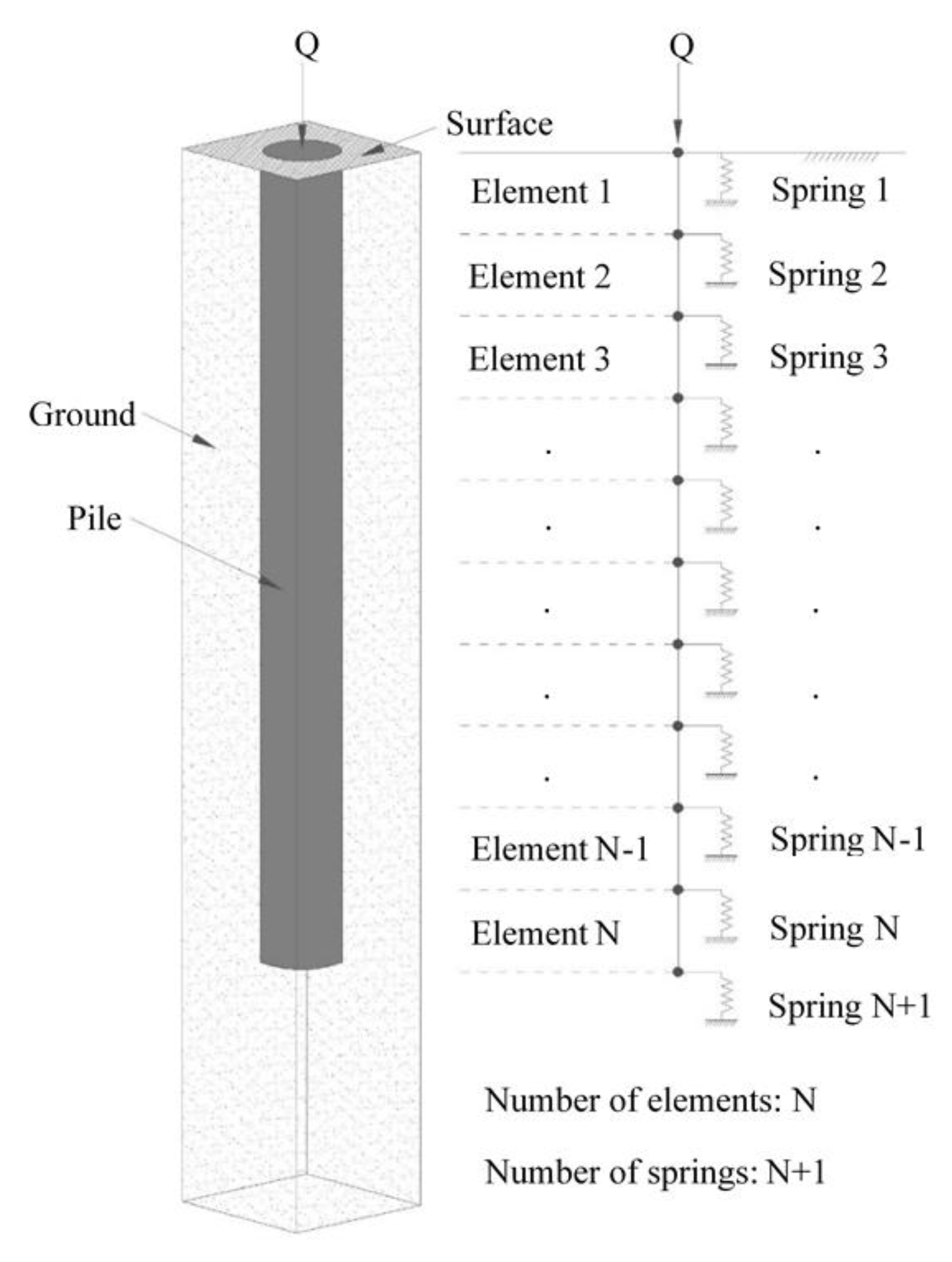
2. Brief Description of the Procedure Followed
- and are the spring stiffness and strength contributions from the soil per unit length along the pile respectively, and
- is the stiffness of the pile.
- have the function to virtually sample soil stiffness , soil strength , and pile stiffness values from specific points or domains (it is noted that the soil consists of a single material, i.e., there is no stratification; the same for the pile),
- calculate the average of the sampled values (when the sampling points are greater than one),
- calculate the resistance of the pile in both the SLS and ULS states, using the sampled value(s) and
- calculate the failure probability of the pile in either the SLS or the ULS state.
- the “optimal sampling strategy” refers to the number of sampling points and their location resulting in an optimal design. In an “optimal design” the error due to a non-effective sampling strategy is the minimum possible (i.e., the statistical uncertainty is minimized). The error is quantified comparing the probability of failure obtained by different sampling scenarios. The term “sampling” may refer to undisturbed specimens or to continuous probing test data (e.g., CPT, SPT).
- In each RFEM realization, “failure” is considered to have occurred when the calculated shaft resistance of the pile considering spatially uniform properties sampled from the soil and pile random fields (average values) is greater than that considering spatially random properties for both the soil and pile.
- The “probability of failure” is defined by the fraction of the realizations resulting in failure relative to the total number of realizations.
3. Parametric Study for Determining the Optimal Sampling Strategy
3.1. Sampling Soil and Pile Properties from a Single Point
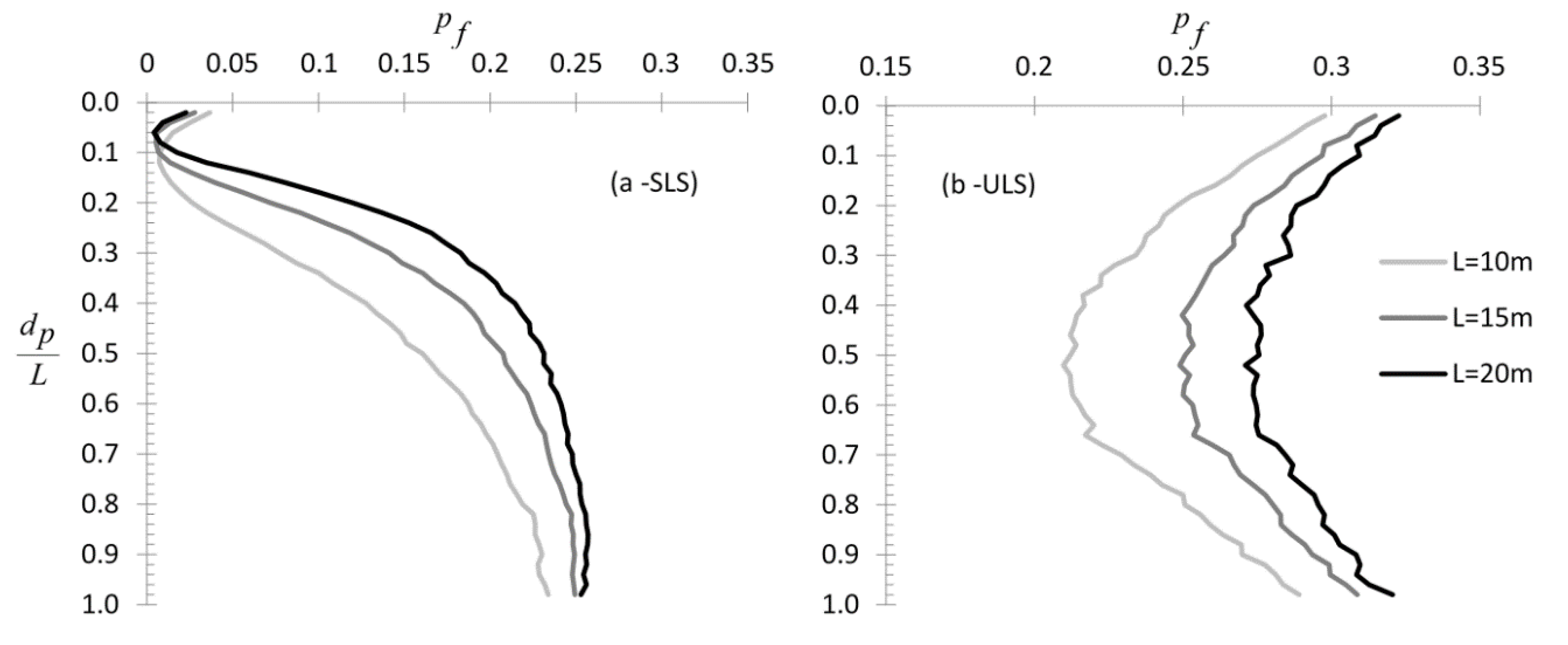
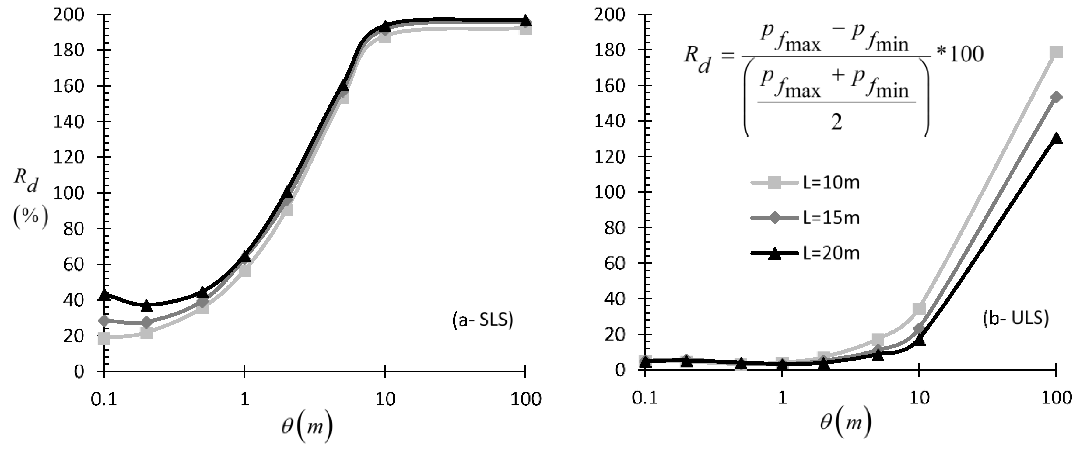
3.1.1. Effect of Spatial Correlation Length and Pile Length
3.1.2. Effect of
3.1.3. Effect of Pile Stiffness
3.1.4. Effect of Soil Stiffness
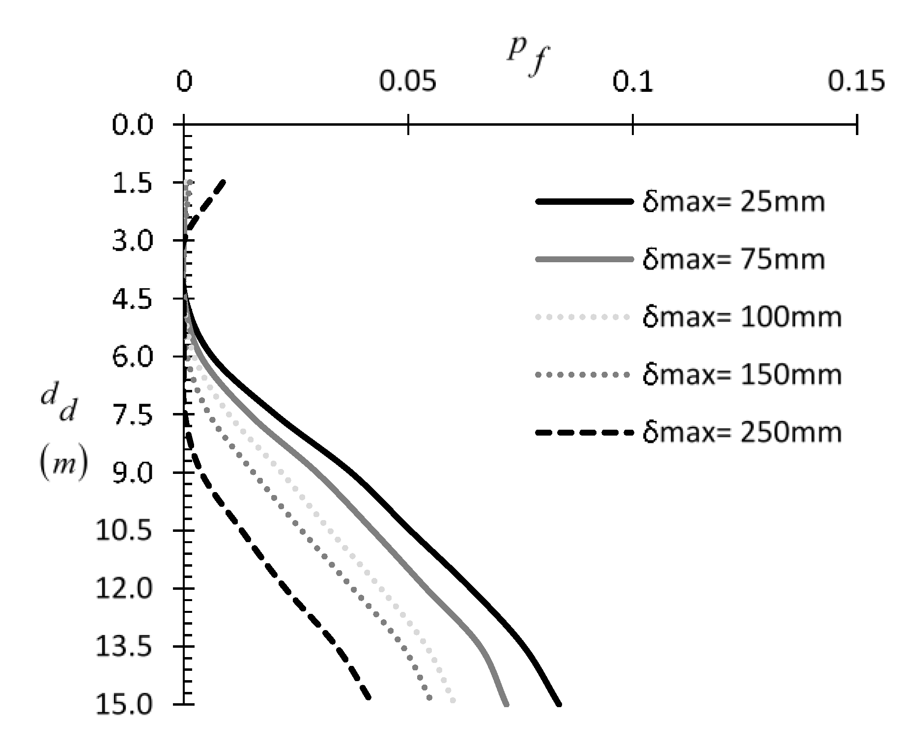
3.1.5. Effect of Soil Strength
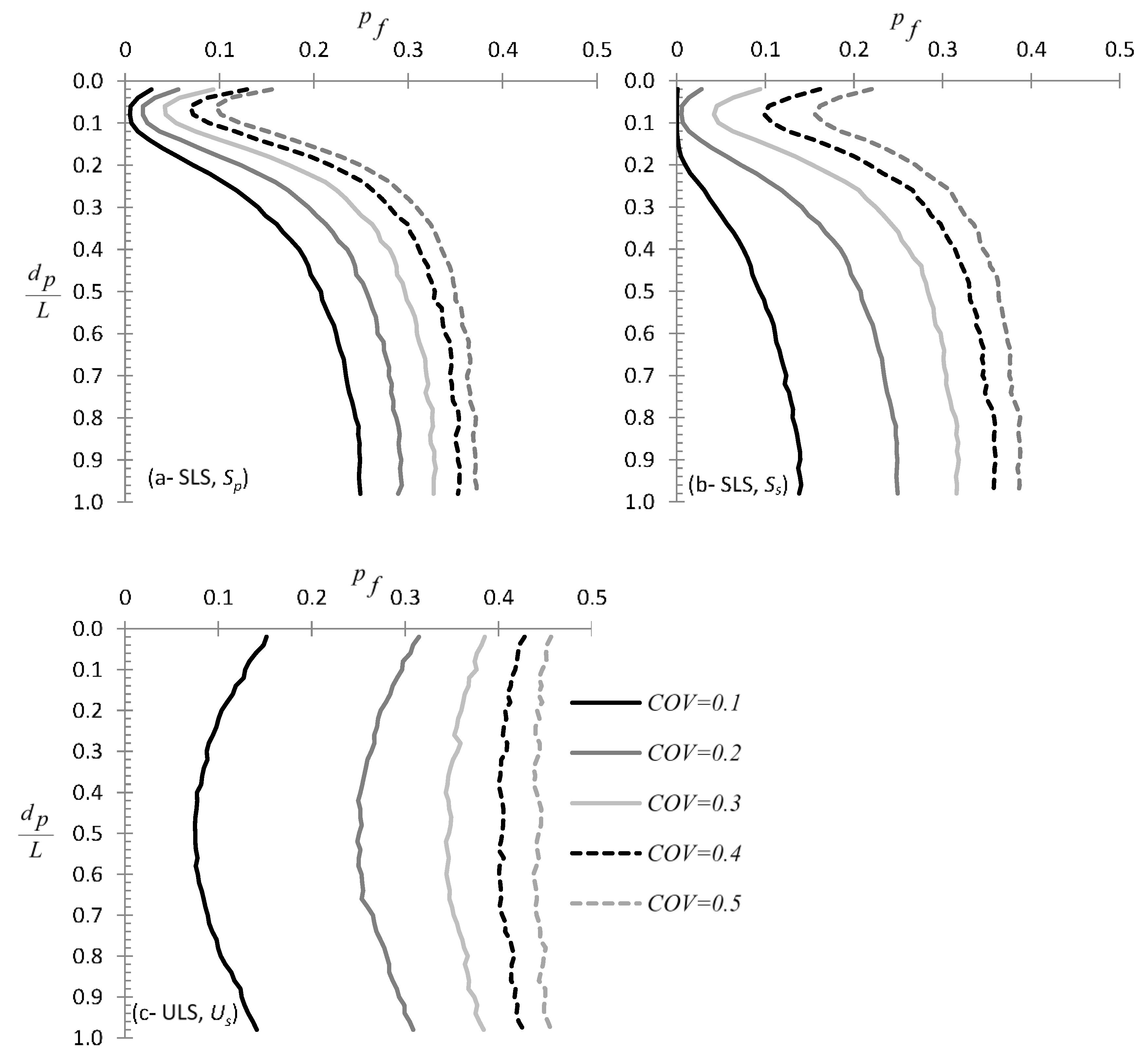
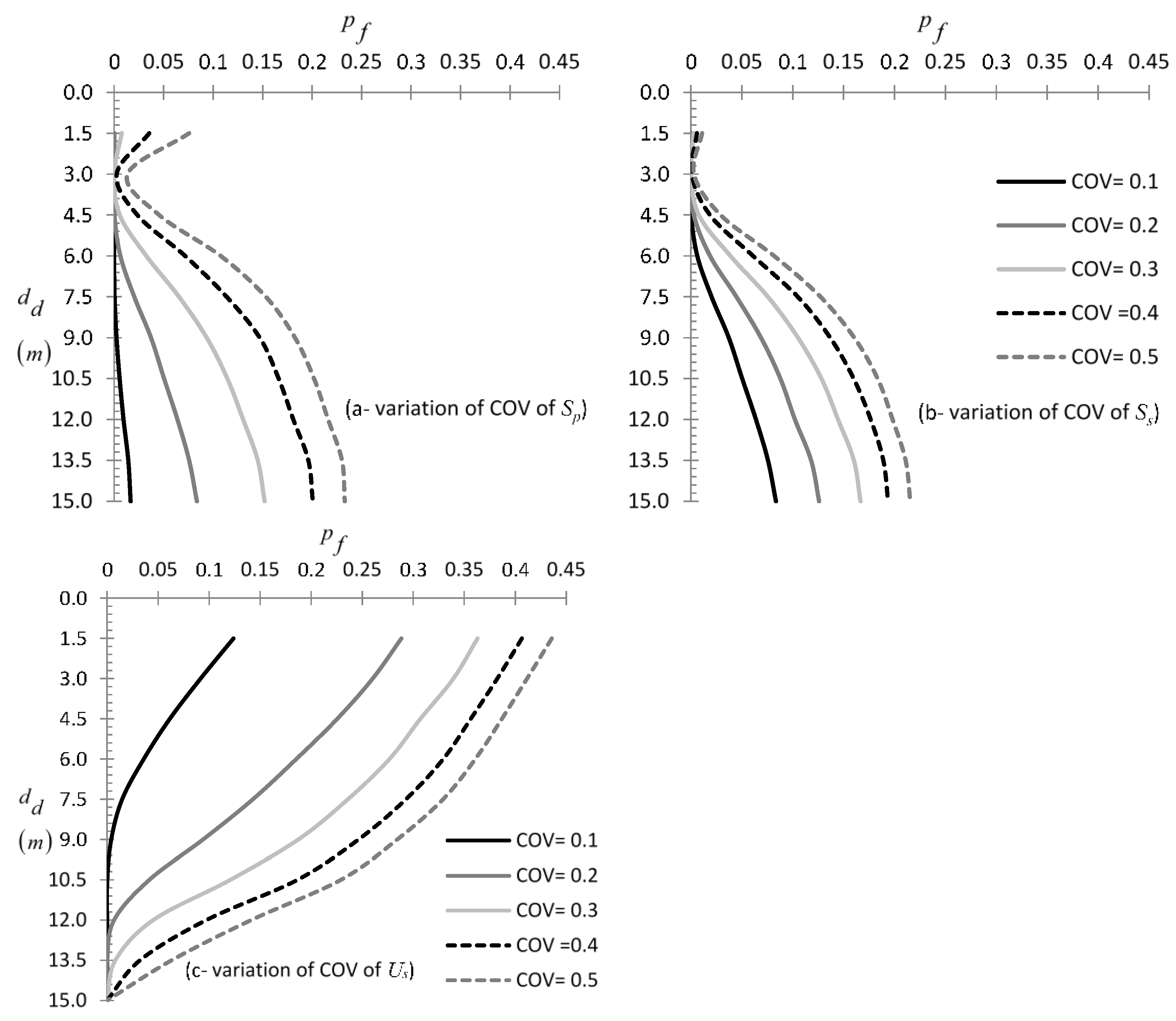
3.1.6. Effect of COV of Pile Stiffness , Soil Stiffness , and Soil Strength
3.2. Sampling Soil and Pile Properties from a Domain
3.2.1. Effect of Pile Stiffness
3.2.2. Effect of Soil Stiffness
3.2.3. Effect of Soil Strength
3.2.4. Effect of
3.2.5. Effect of COV of Pile Stiffness , Soil Stiffness , and Soil Strength
4. The Importance of Targeted Field Investigation in Practice
5. Designing with the Limit State Method
6. Summary and Conclusions
- When continuous probing test data are used and the pile stiffness is much greater than the stiffness of the surrounding soil, the entire pile length is advised to be taken into account both in the and the state, as shorter sampling domain lengths may result in high statistical error.
- Weak piles, such as timber piles, require much shorter domain lengths (measured from the top), as longer sampling domains may increase the error.
- When the design is based on sampling points and not on continuous probing test data, the best practice for minimizing the statistical error is sampling from the mid-height of the pile in both and states.
- When the pile is relatively weak, the optimal sampling point for the state lies near the top of the pile. For the state, the optimal sampling point lies at the mid-height of pile, for any pile stiffness.
- The optimal sampling location in plan-view is the actual location of each pile; by sampling away from this location, high statistical error may be introduced in the analysis.
Author Contributions
Funding
Acknowledgments
Conflicts of Interest
Notation List
| A | pile cross-sectional area |
| smaller side of the rectangle circumscribing the group of piles forming the foundation at the level of the pile base | |
| COV | coefficient of variation |
| pile base diameter | |
| sampling domain length measured from the uppermost point of the pile | |
| depth of the sampling point | |
| modulus of elasticity of the pile | |
| soil’s modulus of elasticity | |
| earth pressure coefficient | |
| coefficient of earth pressure at rest | |
| pile length | |
| number of samples | |
| perimeter of the pile | |
| probability of failure of the pile | |
| maximum probability of failure of the pile | |
| minimum probability of failure of the pile | |
| shaft resistance of the pile | |
| R | pile radius |
| relative percentage difference | |
| serviceability limit state | |
| pile stiffness | |
| soil stiffness | |
| sample standard deviation | |
| Student’s t factor for a confidence level of α% in the case of degrees of freedom | |
| ultimate limit state | |
| soil strength | |
| location where the pile is going to be constructed | |
| characteristic value | |
| sample mean | |
| depth of investigation below the ground level | |
| empirical adhesion factor | |
| adhesion at depth z | |
| soil–pile friction angle | |
| maximum allowable settlement of the pile | |
| spatial correlation length; it refers to both soil and pile properties | |
| mean pile stiffness | |
| mean soil stiffness | |
| mean soil strength | |
| normal effective stress at depth z | |
| average effective overburden pressure | |
| drained friction angle | |
| mean of the sampled drained friction angle | |
| interface friction angle at depth z |
Appendix A. Stability of Numerical Results (Number of Realizations Considered in the RFEM Models)

References
- Griffiths, D.V.; Fenton, G.A.; Ziemann, H.R. Reliability of passive earth pressure. Georisk 2008, 2, 113–121. [Google Scholar] [CrossRef]
- Gong, W.; Luo, Z.; Juang, C.H.; Huang, H.; Zhang, J.; Wang, L. Optimization of site exploration program for improved prediction of tunneling-induced ground settlement in clays. Comput. Geotech. 2014, 56, 69–79. [Google Scholar] [CrossRef]
- Christodoulou, P.; Pantelidis, L.; Gravanis, E. The Effect of Targeted Field Investigation on the Reliability of Earth-Retaining Structures in Active State. Appl. Sci. 2019, 9, 4953. [Google Scholar] [CrossRef] [Green Version]
- Christodoulou, P.; Pantelidis, L.; Gravanis, E. The Effect of Targeted Field Investigation on the Reliability of Earth-Retaining Structures in Passive State: A Random Field Approach. Geosciences 2020, 10, 110. [Google Scholar] [CrossRef] [Green Version]
- Christodoulou, P.; Pantelidis, L. Reducing Statistical Uncertainty in Elastic Settlement Analysis of Shallow Foundations Relying on Targeted Field Investigation: A Random Field Approach. Geosciences 2020, 10, 20. [Google Scholar] [CrossRef] [Green Version]
- Crisp, M.; Jaksa, M.; Kuo, Y.; Fenton, G.A.; Griffiths, V. Characterising Site Investigation Performance in a Two Layer Soil Profile. Can. J. Civ. Eng. 2020. [Google Scholar] [CrossRef]
- Goldsworthy, J.S.; Jaksa, M.B.; Fenton, G.A.; Kaggwa, W.S.; Griffiths, V.; Poulos, H.G. Effect of sample location on the reliability based design of pad foundations. Georisk 2007, 1, 155–166. [Google Scholar] [CrossRef]
- Loehr, J.E.; Ding, D.; Likos, W.J. Effect of number of soil strength measurements on reliability of spread footing designs. Transp. Res. Rec. 2015, 2511, 37–44. [Google Scholar] [CrossRef]
- Jaksa, M.B.; Goldsworthy, J.S.; Fenton, G.A.; Kaggwa, W.S.; Griffiths, D.V.; Kuo, Y.L.; Poulos, H.G. Towards reliable and effective site investigations. Géotechnique 2005, 55, 109–121. [Google Scholar] [CrossRef]
- Mašín, D. The influence of experimental and sampling uncertainties on the probability of unsatisfactory performance in geotechnical applications. Géotechnique 2015, 65, 897–910. [Google Scholar] [CrossRef]
- Li, Y.J.J.; Hicks, M.A.A.; Vardon, P.J.J. Uncertainty reduction and sampling efficiency in slope designs using 3D conditional random fields. Comput. Geotech. 2016, 79, 159–172. [Google Scholar] [CrossRef] [Green Version]
- Yang, R.; Huang, J.; Griffiths, D.V.; Sheng, D. Probabilistic Stability Analysis of Slopes by Conditional Random Fields. Geo-Risk 2017, 2017, 450–459. [Google Scholar]
- Ching, J.; Phoon, K.-K. Characterizing uncertain site-specific trend function by sparse Bayesian learning. J. Eng. Mech. 2017, 143, 4017028. [Google Scholar] [CrossRef]
- Fenton, G.A.; Naghibi, F.; Hicks, M.A. Effect of sampling plan and trend removal on residual uncertainty. Georisk Assess. Manag. Risk Eng. Syst. Geohazards 2018, 12, 253–264. [Google Scholar] [CrossRef]
- Lo, M.K.; Leung, Y.F. Reliability Assessment of Slopes Considering Sampling Influence and Spatial Variability by Sobol’Sensitivity Index. J. Geotech. Geoenviron. Eng. 2018, 144, 4018010. [Google Scholar] [CrossRef]
- Yang, R.; Huang, J.; Griffiths, D.V.; Li, J.; Sheng, D. Importance of soil property sampling location in slope stability assessment. Can. Geotech. J. 2019, 56, 335–346. [Google Scholar] [CrossRef]
- EN. 1997-2 Eurocode 7-Geotechnical Design-Part 2: Ground Investigation and Testing; CEN (European Committee for Standardization): Brussels, Belgium, 2007. [Google Scholar]
- AASHTO. AASHTO LRFD Bridge. Design Specifications; American Association of State Highway and Transportation Officials: Washington, DC, USA, 2010; ISBN 9781560514510. [Google Scholar]
- Sabatini, P.J.; Bachus, R.C.; Mayne, P.W.; Schneider, J.A.; Zettler, T.E. Geotechnical Engineering Circular 5 (GEC5)-Evaluation of Soil and Rock Properties; Report No. FHWA-IF-02-034; Federal Highway Administration, US Department of of Transportation: Washington, DC, USA, 2002.
- Fenton, G.; Griffiths, D.V. Risk Assessment in Geotechnical Engineering; Wiley: Hoboken, NJ, USA, 2008; ISBN 9780470178201. [Google Scholar]
- Fenton, G.A.; Griffiths, D.V. Reliability-based deep foundation design. In Probabilistic Applications in Geotechnical Engineering; Springer Science & Business Media: Berlin/Heidelberg, Germany, 2007; pp. 1–12. [Google Scholar]
- Pacheco, J.; de Brito, J.; Chastre, C.; Evangelista, L. Experimental investigation on the variability of the main mechanical properties of concrete produced with coarse recycled concrete aggregates. Constr. Build. Mater. 2019, 201, 110–120. [Google Scholar] [CrossRef]
- Aït-Mokhtar, A.; Belarbi, R.; Benboudjema, F.; Burlion, N.; Capra, B.; Carcasses, M.; Colliat, J.-B.; Cussigh, F.; Deby, F.; Jacquemot, F. Experimental investigation of the variability of concrete durability properties. Cem. Concr. Res. 2013, 45, 21–36. [Google Scholar] [CrossRef] [Green Version]
- Christou, G.; Tantele, E.A.; Votsis, R.A. Effect of environmental deterioration on buildings: A condition assessment case study. In Proceedings of the RSCy2014, Paphos, Cyprus, 7–10 April 2014; International Society for Optics and Photonics: Bellingham, WA, USA, 2014; Volume 9229, p. 92290. [Google Scholar]
- Masi, A.; Chiauzzi, L. An experimental study on the within-member variability of in situ concrete strength in RC building structures. Constr. Build. Mater. 2013, 47, 951–961. [Google Scholar] [CrossRef]
- Wood, L.W. Variation of Strength Properties in Woods Used for Structural Purposes; USDA Forest Service: Washington, DC, USA, 1960.
- Das, B.M. Principle of Geotechnical Engineering, 7th ed.; Cengage Learning: Stamford, CT, USA, 2010; ISBN 9780495668121. [Google Scholar]
- Venkatramaiah, C. Geotechnical Engineering; New Age International: New Delhi, India, 2006; ISBN 812240829X. [Google Scholar]
- Canadian Standards Association Canadian Highway Bridge. Design Code. CAN/CSA-S6-14; Canadian Standards Association: Mississauga, ON, Canada, 2014. [Google Scholar]
- Kok-Kwang, P.; Kulhawy, F.H.; Grigoriu, M.D. Development of a Reliability-Based Design Framework for Transmission Line Structure Foundations. J. Geotech. Geoenvironm. Eng. 2003, 129, 798–806. [Google Scholar]
- Fenton, G.A.; Naghibi, F.; Dundas, D.; Bathurst, R.J.; Griffiths, D.V. Reliability-based geotechnical design in 2014 Canadian Highway Bridge Design Code. Can. Geotech. J. 2015, 53, 236–251. [Google Scholar] [CrossRef]
- EN. 1997-1 Eurocode 7 Geotechnical Design—Part 1: General Rules; CEN (European Committee for Standardization): Brussels, Belgium, 2004. [Google Scholar]
- JGS Principles for Foundation Design Grounded on a Performance-Based Design Concept (GeoGuide); Japanese Geotechnical Society: Tokyo, Japan, 2004.
- Orr, T.L.L. Defining and selecting characteristic values of geotechnical parameters for designs to Eurocode 7. Georisk Assess. Manag. Risk Eng. Syst. Geohazards 2016, 11, 103–115. [Google Scholar] [CrossRef]
- Vanmarcke, E.H. Reliability of earth slopes. J. Geotech. Eng. Div. 1977, 103, 1247–1265. [Google Scholar]
- Soulie, M.; Montes, P.; Silvestri, V. Modelling spatial variability of soil parameters. Can. Geotech. J. 1990, 27, 617–630. [Google Scholar] [CrossRef]
- Cherubini, C. Data and considerations on the variability of geotechnical properties of soils. In Proceedings of the International Conference on Safety and Reliability, ESREL, Lisbon, Portugal, 17–20 June 1997; Volume 97, pp. 1583–1591. [Google Scholar]
- Popescu, R.; Prévost, J.H.; Deodatis, G. Effects of spatial variability on soil liquefaction: Some design recommendations. Geotechnique 1997, 47, 1019–1036. [Google Scholar] [CrossRef]
- Phoon, K.; Kulhawy, F. Characterization of geotechnical variability. Can. Geotech. J. 1999, 36, 612–624. [Google Scholar] [CrossRef]
- Christodoulou, P.; Pantelidis, L.; Gravanis, E. A Comparative Assessment of the Methods-of-Moments for Estimating the Correlation Length of One-Dimensional Random Fields. Arch. Comput. Methods Eng. 2020. [Google Scholar] [CrossRef]


| COV | COV | COV | ||||
|---|---|---|---|---|---|---|
| 25 mm | 1000 kN | 0.1 | 100 kN/m/m | 0.2 | 10 kN/m | 0.2 |
| Example | Random Field | Distribution | Figure | ||||
|---|---|---|---|---|---|---|---|
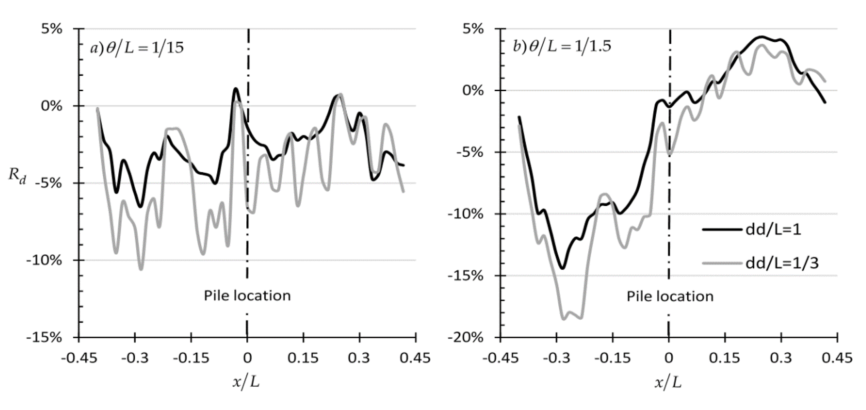
| #1 | Log-normal | 30° | 0.2 | 15 | 1/15 | 10a | |
| #2 | Log-normal | 30° | 0.2 | 15 | 1/1.5 | 10b |
© 2020 by the authors. Licensee MDPI, Basel, Switzerland. This article is an open access article distributed under the terms and conditions of the Creative Commons Attribution (CC BY) license (http://creativecommons.org/licenses/by/4.0/).
Share and Cite
Christodoulou, P.; Pantelidis, L.; Gravanis, E. The Effect of Targeted Field Investigation on the Reliability of Axially Loaded Piles: A Random Field Approach. Geosciences 2020, 10, 160. https://doi.org/10.3390/geosciences10050160
Christodoulou P, Pantelidis L, Gravanis E. The Effect of Targeted Field Investigation on the Reliability of Axially Loaded Piles: A Random Field Approach. Geosciences. 2020; 10(5):160. https://doi.org/10.3390/geosciences10050160
Chicago/Turabian StyleChristodoulou, Panagiotis, Lysandros Pantelidis, and Elias Gravanis. 2020. "The Effect of Targeted Field Investigation on the Reliability of Axially Loaded Piles: A Random Field Approach" Geosciences 10, no. 5: 160. https://doi.org/10.3390/geosciences10050160
APA StyleChristodoulou, P., Pantelidis, L., & Gravanis, E. (2020). The Effect of Targeted Field Investigation on the Reliability of Axially Loaded Piles: A Random Field Approach. Geosciences, 10(5), 160. https://doi.org/10.3390/geosciences10050160