Analysis of Very High Spatial Resolution Images for Automatic Shoreline Extraction and Satellite-Derived Bathymetry Mapping †


Abstract
:1. Introduction
2. Materials and Methods
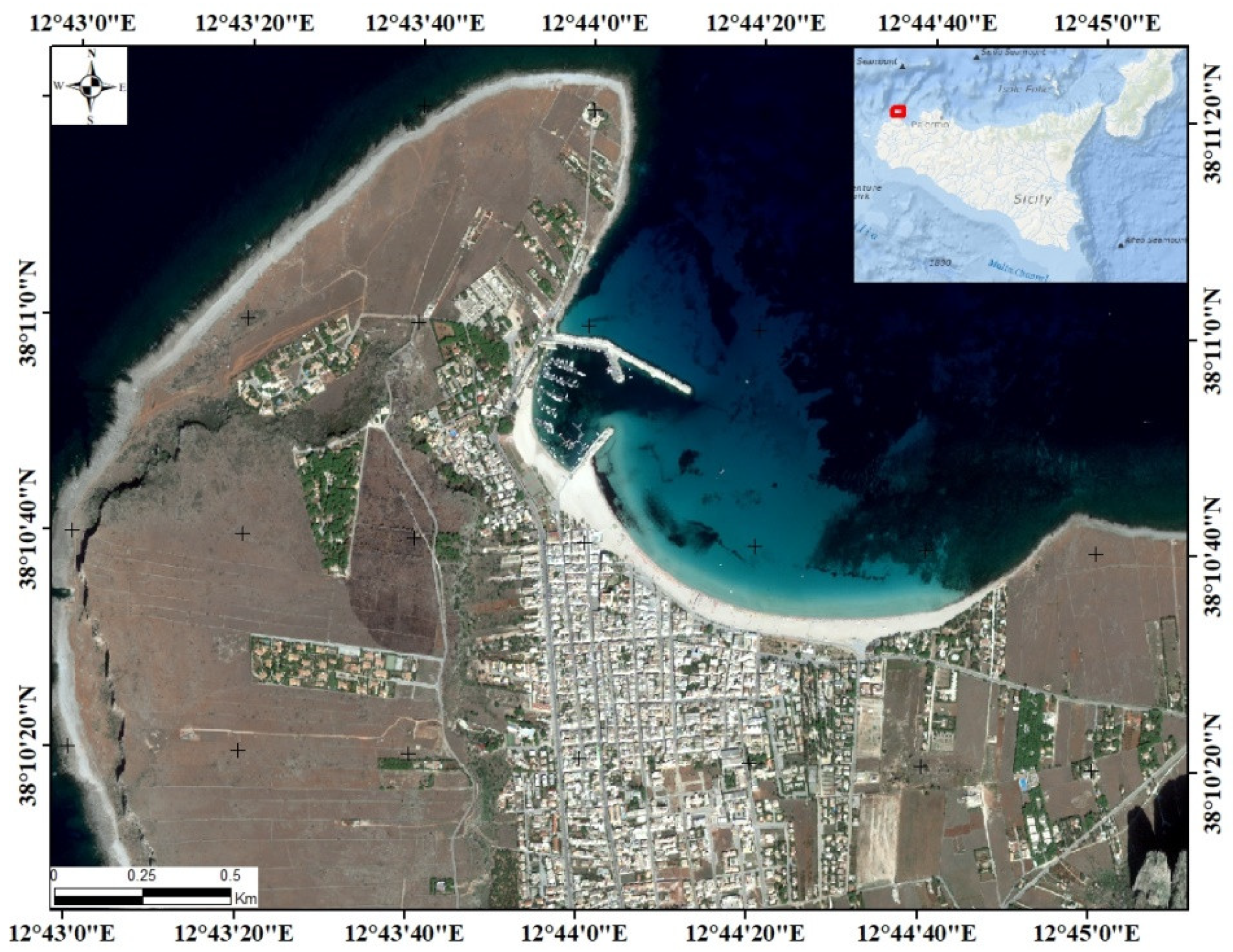
2.1. Area of Study
2.2. Data Used
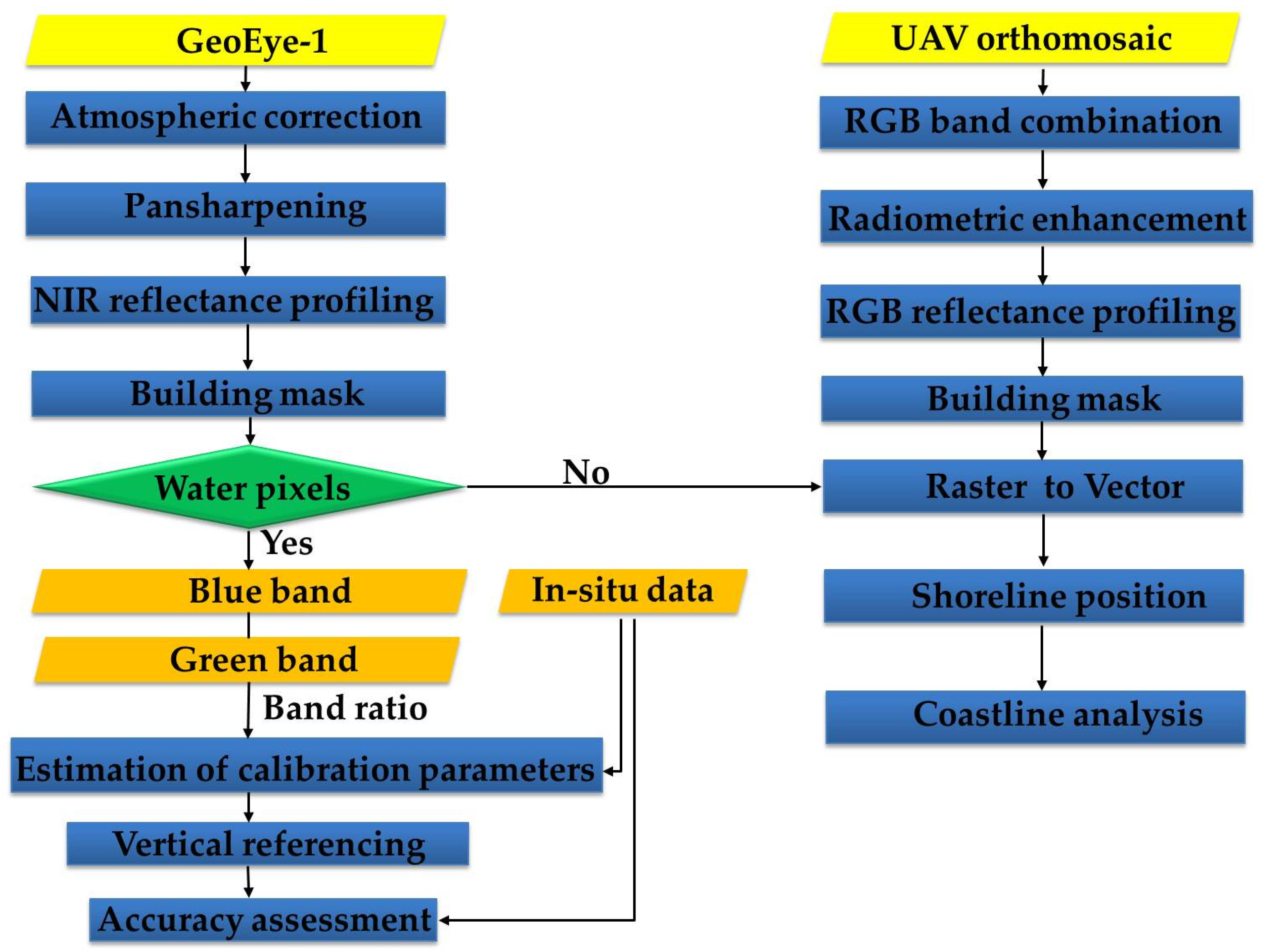
2.3. Methodology
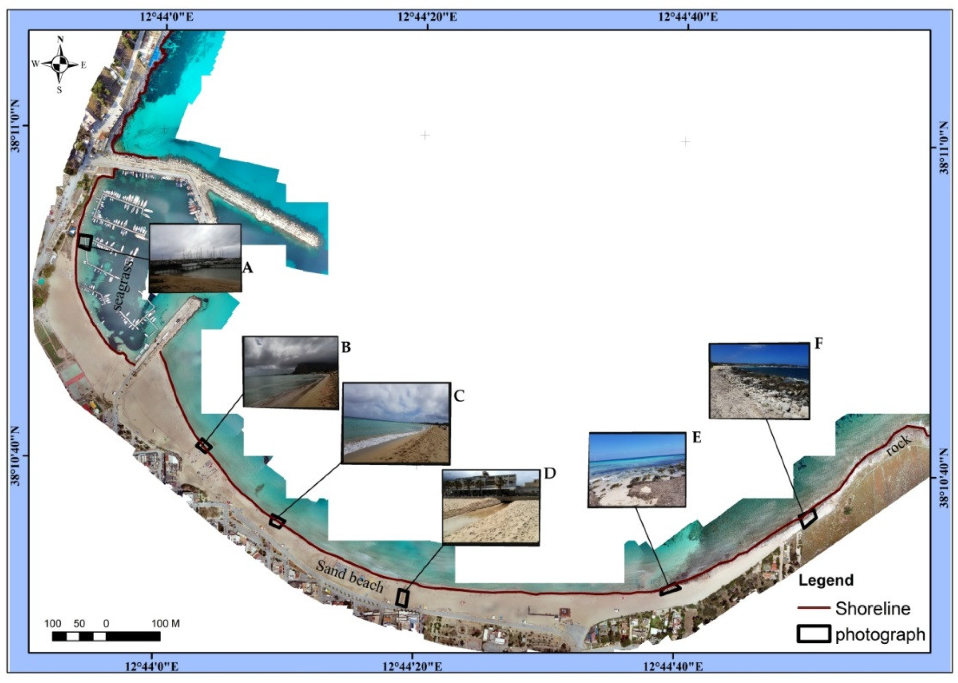
2.3.1. Automatic Shoreline Extraction
2.3.2. Satellite-derived Bathymetry
3. Results
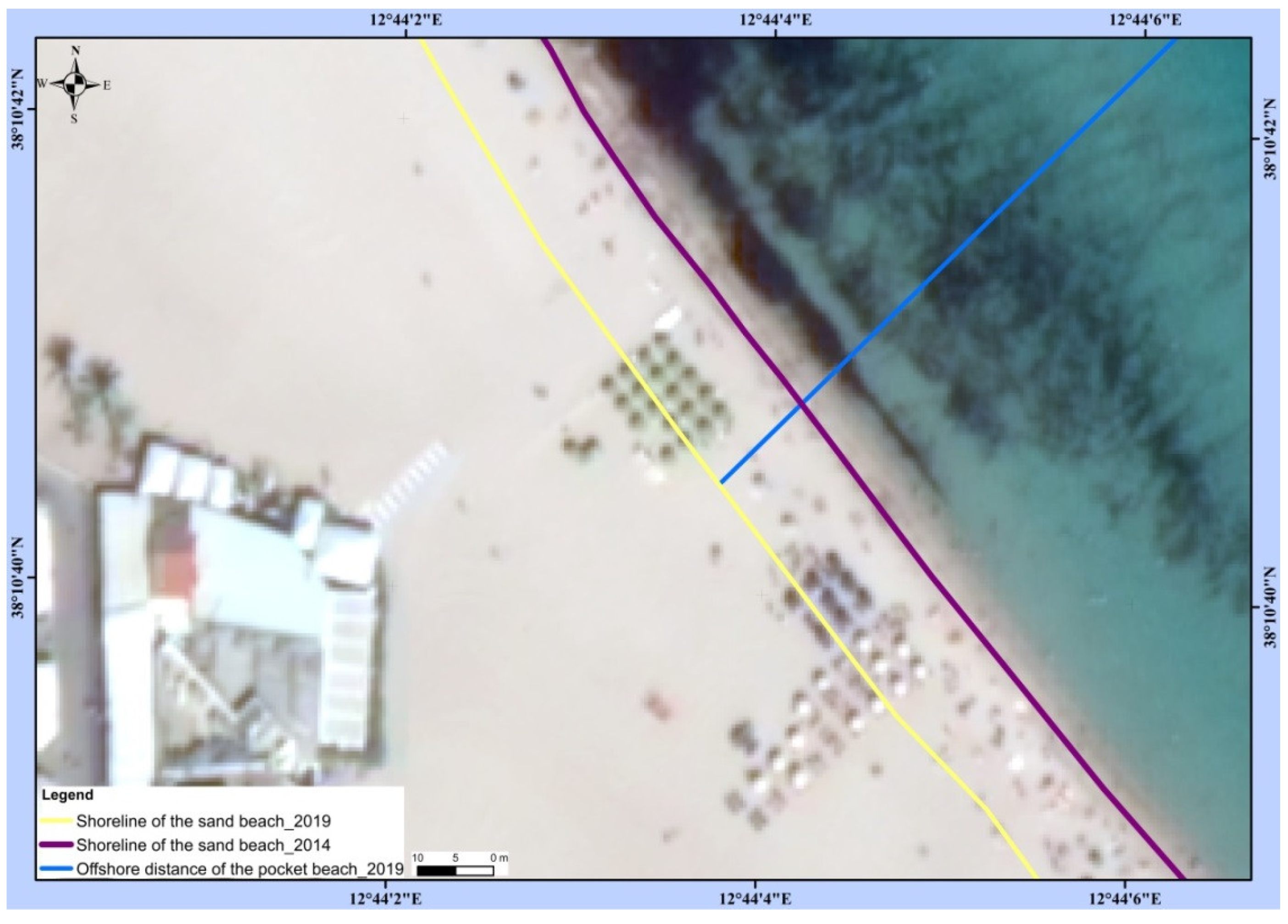
3.1. Shoreline Variability
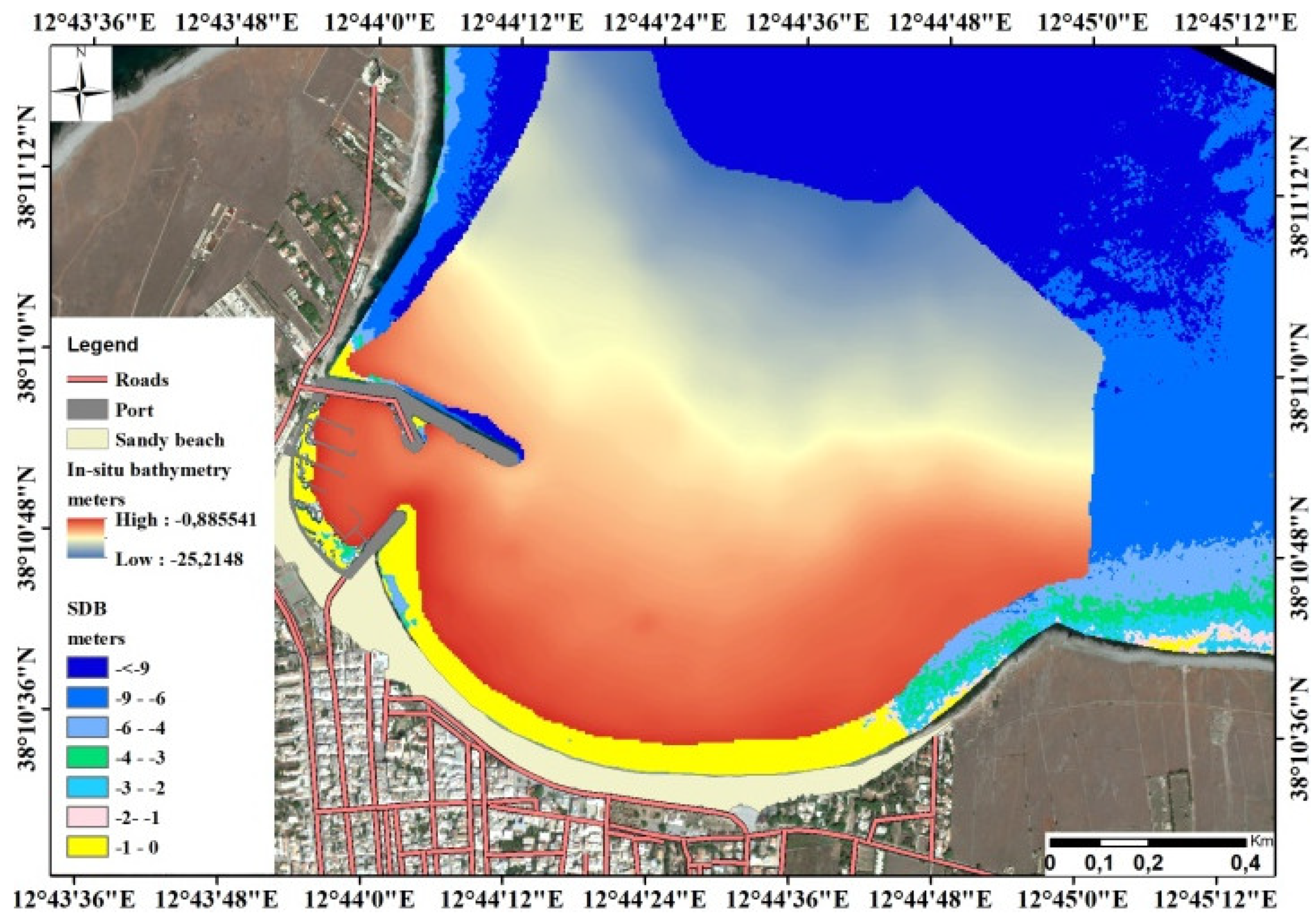
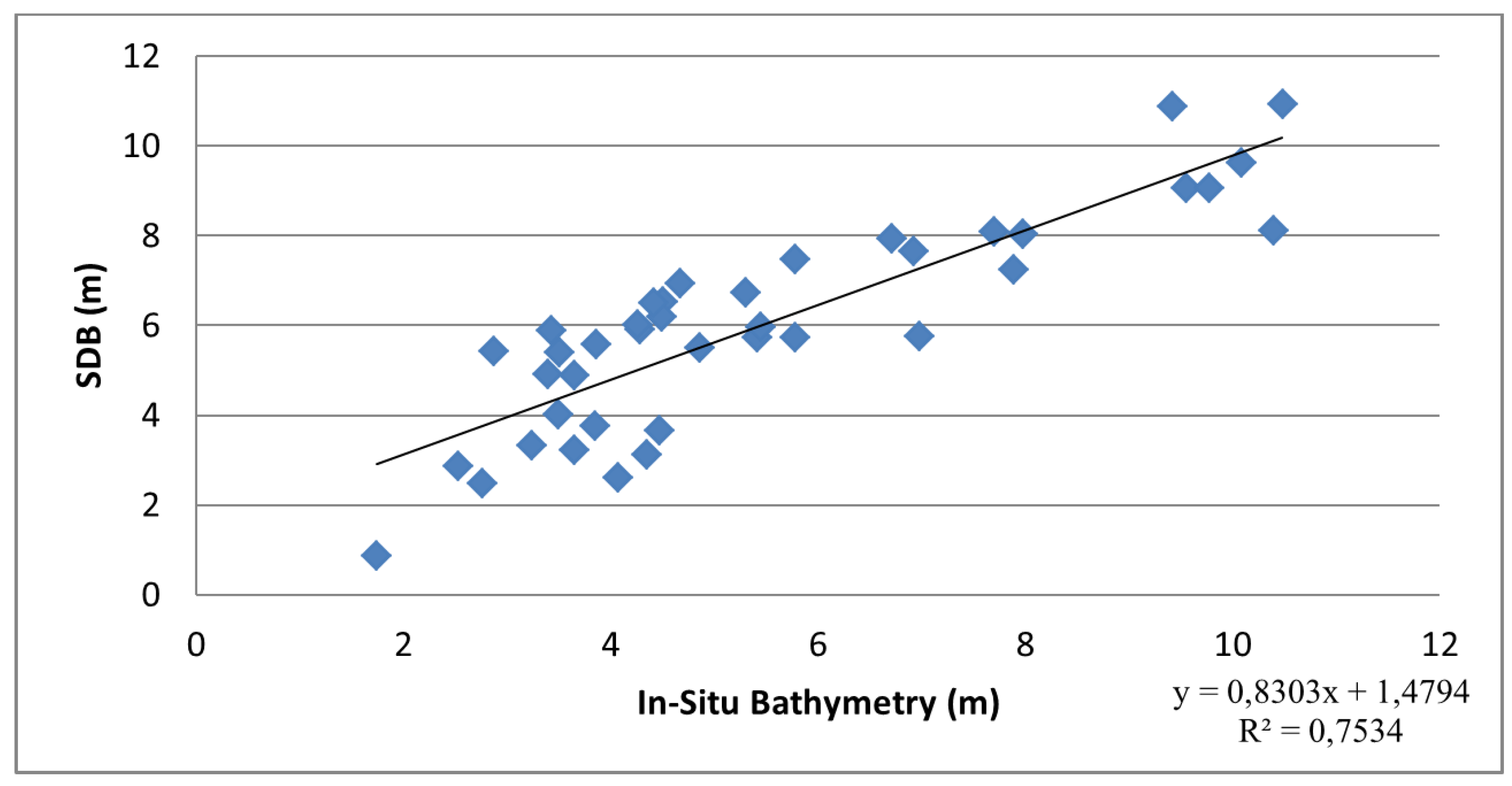
3.2. Satellite-derived Bathymetry
4. Discussion
4.1. Automatic Shoreline Extraction on GeoEye-1 Satellite and UAV Orthomosaic Images
4.2. Satellite-derived Bathymetry Mapping
5. Conclusions
Author Contributions
Funding
Acknowledgments
Conflicts of Interest
References
- Conti, L.A. Coastline changes near the “Maranhão-Ponta da Madeira” Port Complex, Brazil. J. Integ. Coast. Zone Manag. 2019, 19, 71–84. [Google Scholar] [CrossRef]
- Braga, F.; Tosi, L.; Prati, C.; Alberotanza, L. Shoreline detection: Capability of COSMO-SkyMed and high-resolution multispectral images. Eur. J. Remote Sens. 2013, 46, 837–853. [Google Scholar] [CrossRef]
- Maglione, P.; Parente, C.; Vallario, A. High Resolution Satellite Images to Reconstruct Recent Evolution of Domitian Coastline. Am. J. Appl. Sci. 2015, 12, 506–515. [Google Scholar] [CrossRef] [Green Version]
- Rishikeshan, C.A.; Ramesh, H. A novel mathematical morphology based algorithm for shoreline extraction from satellite images. Geo-spat. inf. Sci. 2017, 20, 345–352. [Google Scholar] [CrossRef] [Green Version]
- Chen, B.; Yang, Y.; Xu, D.; Huang, E. A dual band algorithm for shallow water depth retrieval from high spatial resolution imagery with no ground truth. ISPRS J. Photo. Remote Sens. 2019, 151, 1–13. [Google Scholar] [CrossRef]
- Hassler, S.C.; Baysal-Gurel, F. Unmanned Aircraft System (UAS) Technology and Applications in Agriculture. Agronomy 2019, 9, 618. [Google Scholar] [CrossRef] [Green Version]
- Laporte-Fauret, Q.; Marieu, V.; Castelle, B.; Michalet, R.; Bujan, S.; Rosebery, D. Low-Cost UAV for High-Resolution and Large-Scale Coastal Dune Change Monitoring Using Photogrammetry. J. Mar. Sci. Eng. 2019, 7, 63. [Google Scholar] [CrossRef] [Green Version]
- Agrafiotis, P.; Skarlatos, D.; Georgopoulos, A.; Karantzalos, K. Shallow water bathymetry mapping from UAV imagery based on machine learning. arXiv 2019, arXiv:1902.10733. [Google Scholar] [CrossRef] [Green Version]
- Pellicani, R.; Argentiero, I.; Manzari, P.; Spilotro, G.; Marzo, C.; Ermini, R.; Apollonio, C. UAV and Airborne LiDAR Data for Interpreting Kinematic Evolution of Landslide Movements: The Case Study of the Montescaglioso Landslide (Southern Italy). Geosciences 2019, 9, 248. [Google Scholar] [CrossRef] [Green Version]
- Reimann, L.; Vafeidis, A.T.; Brown, S.; Hinkel, J.; Tol, R.S.J. Mediterranean UNESCO World Heritage at risk from coastal flooding and erosion due to sea-level rise. Nat. Commun. 2018, 9, 4161. [Google Scholar] [CrossRef] [PubMed] [Green Version]
- Nikolakopoulos, K.; Kyriou, A.; Koukouvelas, I.; Zygouri, V.; Apostolopoulos, D. Combination of Aerial, Satellite, and UAV Photogrammetry for Mapping the Diachronic Coastline Evolution: The Case of Lefkada Island. ISPRS Int. J. Geo-Inf. 2019, 8, 489. [Google Scholar] [CrossRef] [Green Version]
- Klemas, V. The role of remote sensing in predicting and determining coastal storm impacts. J. Coast. Res. 2009, 6, 1264–1275. [Google Scholar] [CrossRef] [Green Version]
- Sudmanns, M.; Tiede, D.; Lang, S.; Bergstedt, H.; Trost, G.; Augustin, H.; Baraldi, A.; Blaschke, T. Big Earth data: Disruptive changes in Earth observation data management and analysis? Int. J. Digit. Earth 2019, 1–19. [Google Scholar] [CrossRef]
- Lou, X.; Huang, W.; Shi, A.; Teng, J. Raster to vector conversion of classified remote sensing image. In Proceedings of the 2005 IEEE International Geoscience and Remote Sensing Symposium IGARSS-05, Seoul, Korea, 29 July 2005; Volume 5, pp. 3656–3658. [Google Scholar]
- Guariglia, A.; Buonamassa, A.; Losurdo, A.; Saladino, R.; Trivigno, M.L.; Zaccagnino, A.; Colangelo, A. A Multisource Approach for Coastline Mapping and Identification of Shoreline Changes. Ann. Geophys. 2006, 41, 295–304. [Google Scholar]
- Gesch, D.; Wilson, R. Development of a seamless multisource topographic/bathymetric elevation model of Tampa Bay. Mar. Technol. Soc. J. 2002, 35, 58–64. [Google Scholar] [CrossRef] [Green Version]
- Monteys, X.; Harris, P.; Caloca, S.; Cahalane, C. Spatial Prediction of Coastal Bathymetry Based on Multispectral Satellite Imagery and Multibeam Data. Remote Sens. 2015, 7, 13782–13806. [Google Scholar] [CrossRef] [Green Version]
- Muzirafuti, A.; Barreca, G.; Crupi, A.; Faina, G.; Paltrinieri, D.; Lanza, S.; Randazzo, G. The Contribution of Multispectral Satellite Image to Shallow Water Bathymetry Mapping on the Coast of Misano Adriatico, Italy. J. Mar. Sci. Eng. 2020, 8, 126. [Google Scholar] [CrossRef] [Green Version]
- Seif, A.K.; Kuroiwa, M.; Abualtayef, M.; Mase, H.; Matsubara, Y. A hydrodynamic model of nearshore waves and wave-induced currents. Inter. J. Nav. Archit. Oc. Engng. 2011, 3, 216–224. [Google Scholar] [CrossRef] [Green Version]
- Clementi, E.; Oddo, P.; Drudi, M.; Pinardi, N.; Korres, G.; Grandi, A. Coupling hydrodynamic and wave models: First step and sensitivity experiments in the Mediterranean Sea. Ocean Dynam. 2017, 67, 1293–1312. [Google Scholar] [CrossRef] [Green Version]
- Van Rijn, L.C. Coastal erosion and control. Ocean Coast. Manag. 2011, 54, 867–887. [Google Scholar] [CrossRef]
- Guzinski, R.; Spondylis, E.; Michalis, M.; Tusa, S.; Brancato, G.; Minno, L.; Hansen, L.B. Exploring the Utility of Bathymetry Maps Derived with Multispectral Satellite Observations in the Field of Underwater Archaeology. Open Archaeol. 2016, 2, 243–263. [Google Scholar] [CrossRef] [Green Version]
- Bannari, A.; Kadhem, G. MBES-CARIS Data Validation for Bathymetric Mapping of Shallow Water in the Kingdom of Bahrain on the Arabian Gulf. Remote Sens. 2017, 9, 385. [Google Scholar] [CrossRef] [Green Version]
- Anderson, J.T.; Van Holliday, D.; Kloser, R.; Reid, D.G.; Simard, Y. Acoustic seabed classification: Current practice and future directions. ICES J. Mar. Sci. 2008, 65, 1004–1011. [Google Scholar] [CrossRef]
- Zhao, J.; Zhao, X.; Zhang, H.; Zhou, F. Shallow Water Measurements Using a Single Green Laser Corrected by Building a Near Water Surface Penetration Model. Remote Sens. 2017, 9, 426. [Google Scholar] [CrossRef] [Green Version]
- Wang, C.K.; Philpot, W.D. Using airborne bathymetric Lidar to detect bottom type variation in shallow waters. Remote Sens. Environ. 2007, 106, 123–135. [Google Scholar] [CrossRef]
- Conner, J.T.; Tonina, D. Effect of cross-section interpolated bathymetry on 2D hydrodynamic results in a large river. Earth Surf. Process. Landf. 2014, 39, 463–475. [Google Scholar] [CrossRef]
- Horritt, M.S.; Bates, P.D.; Mattinson, M.J. Effects of mesh resolution and topographic representation in 2D finite volume models of shallow water fluvial flow. J. Hydrol. 2006, 329, 306–314. [Google Scholar] [CrossRef]
- Chénier, R.; Faucher, M.-A.; Ahola, R. Satellite-Derived Bathymetry for Improving Canadian Hydrographic Service Charts. ISPRS Int. J. Geo-Inf. 2018, 7, 306. [Google Scholar] [CrossRef] [Green Version]
- Polcyn, F.C.; Brown, W.L.; Sattinger, I.J. The Measurement of Water Depth by Remote Sensing Techniques; Report No. 8973-26-F.; Willow Run Laboratories of the Institute of Science and Technology, The University of Michigan: Ann Arbor, MI, USA, 1970. [Google Scholar]
- Siermann, J.; Harvey, C.; Morgan, G.; Heege, T. Satellite derived bathymetry and digital elevation models (DEM). In Proceedings of the International petroleum technology conference, Doha, Qatar, 19–22 January 2014. [Google Scholar]
- EOMAP. “Satellite-Derived Bathymetry”. Available online: https://www.eomap.com/services/bathymetry/ (accessed on 1 September 2019).
- TCARTA. “What is Satellite Derived Bathymetry?”. Available online: https://www.tcarta.com/blog/what-is-satellite-derived-bathymetry/ (accessed on 1 September 2019).
- Mavraeidopoulos, A.K.; Pallikaris, A.; Oikonomou, E. Satellite Derived Bathymetry (SDB) and Safety of Navigation. Int. Hydrogr. Rev. 2017, 17, 7–19. [Google Scholar]
- Basterretxea, G.; Orfica, A.; Jordi, A.; Casas, B.; Lynett, P.; Liu, P.L.F.; Duarte, C.M.; Tintore, J. Seasonal dynamics of a microtidal pocket beach with Posidonia oceanica seabed (Mallorca, Spain). J. Coast. Res. 2004, 20, 1155–1164. [Google Scholar] [CrossRef] [Green Version]
- Schwab, W.C.; Thieler, R.E.; Allen, J.R.; Foster, D.S.; Ann Swift, B.; Denny, J.F. Influence of inner-continental shelf geologic framework on the evolution and behaviour of the barrier-island system between Fire Island Inlet and Shinnecock Inlet, Long Island, New York. J. Coast. Res. 2000, 16, 408–422. [Google Scholar]
- Aguzzi, M.; Bonsignore, F.; De Nunzio, N.; Morelli, M.; Paccagnella, T.; Romagnoli, C.; Unguendoli, S. Stato del Litorale Emiliano-Romagnolo al 2012: Erosione e Interventi di Difesa; Agenzia Prevenzione Ambiente Energia Emilia-Romagna: Bologna, Italy, 2016; ISBN 978-88-87854-41-1. [Google Scholar]
- Muzirafuti, A.; Crupi, A.; Lanza, S.; Barreca, G.; Randazzo, G. Shallow water bathymetry by satellite image: A case study on the coast of San Lo Capo Peninsula, Northwestern Sicily, Italy. In Proceedings of the 2019 IMEKO TC-19 International Workshop on Metrology for the Sea, Genova, Italy, 3–5 October 2019. [Google Scholar]
- IOCCG. Atmospheric Correction for Remotely-Sensed Ocean-Colour Products. In Reports of the International Ocean-Colour Coordinating Group (IOCCG); No. 10; Wang, M., Ed.; International Ocean-Colour Coordinating Group: Dartmouth, NS, Canada, 2010. [Google Scholar]
- Eugenio, F.; Marcello, J.; Martin, J.; Rodríguez-Esparragón, D. Benthic Habitat Mapping Using Multispectral High-Resolution Imagery: Evaluation of Shallow Water Atmospheric Correction Techniques. Sensors 2017, 17, 2639. [Google Scholar] [CrossRef] [PubMed] [Green Version]
- Stumpf, R.P.; Holderied, K.; Sinclair, M. Determination of water depth with high-resolution satellite imagery over variable bottom types. Limnol. Oceanogr. 2003, 48, 547–556. [Google Scholar] [CrossRef]
- Eugenio, F.; Marcello, J.; Martin, J. High-resolution maps of bathymetry and benthic habitats in shallow-water environments using multispectral remote sensing imagery. IEEE Trans. Geosci. Remote Sens. 2015, 53, 3539–3549. [Google Scholar] [CrossRef]


| Image Type | Panchromatic | Multispectral | ||
|---|---|---|---|---|
| Spatial resolution | 0.5 m | 2 m | ||
| Spectral resolution | 450–900 nm | 450–520 nm for the blue band 520–600 nm for the green band 625–695 nm for the red band 760–900 nm for the NIR band | ||
| Image calibration parameter | Gain mw/(cm2 × nm × sr) | Offset | Gain µw/( cm2 × nm × sr) | Offset |
| 0.08715 | 0 | 0.14865 for blue band 0.10135 for green band 0.16194003 for red band 0.05705 for NIR band | 0 0 0 0 | |
| Off-Nadir imaging | 26 degrees | |||
| Coordinate system | WGS 1984 UTM Zone 33N | |||
| Cloud cover | 0 | |||
| Positional Instrument | DGPS Garmin CSX 60 signal differential WAAS EGNOA | |
| Coordinate System | Datum: Roma 1940 (Monte Mario), Projection: ( Gauss Boaga ) | |
| Navigation Software | Qinsy QPS 8.1.0 | |
| Tide Station | National mareographic network_station of Palermo | |
| Date: 07-11-2013 | Date: 08-11-2013 | |
| High value: 0.225 m Low value: −0.024 m | High value: 0.2 m Low value: −0.026 | |
| Bathymetric Map Scale | 1:2250 | |
| Sensing Parameters | DJI Mavic pro 2 Aircraft |
|---|---|
| Sensor type | Camera Hasselblad L1D-20c-20 Mega pix |
| Spatial resolution | 1.58 cm |
| Spectral resolution/number of bands | 3 bands RGB |
| Radiometric resolution | 24 BIT |
| Flight altitude | 60 m |
| Flight duration | 20 minutes |
| Total area covered | 0.62 km2 |
| Forward and sideward overlap sensing | 75% frontal–75% side |
| Flight speed | 5.2 m/s |
| Sensing type | automatic |
| Number of people mobilized | 3 |
| Data and time image acquisition | 28 May 2019, 11: 00 UTC |
| Off-Nadir imaging | 0 degree |
| Coordinate system | WGS84 UTM zone 33 N |
| Image type | GeoTIFF |
| Number of flights | 3 |
| Global navigation satellite system (GNSS) | GPS+GLONASS |
| Band Features | Masking Threshold | Definition | |
|---|---|---|---|
| GeoEye-1 NIR Band | UAV Orthomosaic Red Band | ||
| Land | ≥0.35 | ≥160 | Sand beach and built up area with high values |
| Water | ≤0.35 | ≤160 | Shallow water with low values |
| Coastline Analysis Parameters | Situation in 2014 | Situation in 2019 |
|---|---|---|
| Shoreline of the sand beach (m) | 1776 | 1879 |
| Distance of the beach (m) | 1486 | 1496 |
| Offshore distance of the pocket beach (m) | 936 | 951 |
| Headland spacing (m) | 1772 | 1772 |
| Total length of shoreline (m) | 3376 | 3451 |
| Near shoreline eroded surface (m2) | 17,446 | |
| Near shoreline gained surface | 695 | |
| Sand beach surface (m2) | 99,810 | 84,360 |
| Depth Range (m) | Error (m) |
|---|---|
| 1–2 | −0.85 |
| 2–3 | 0.98 |
| 3–4 | 1.01 |
| 4–5 | 0.87 |
| 5–6 | 0.79 |
| 6–7 | 0.27 |
| 7–9 | 0.02 |
| 9–10 | −0.75 |
© 2020 by the authors. Licensee MDPI, Basel, Switzerland. This article is an open access article distributed under the terms and conditions of the Creative Commons Attribution (CC BY) license (http://creativecommons.org/licenses/by/4.0/).
Share and Cite
Randazzo, G.; Barreca, G.; Cascio, M.; Crupi, A.; Fontana, M.; Gregorio, F.; Lanza, S.; Muzirafuti, A. Analysis of Very High Spatial Resolution Images for Automatic Shoreline Extraction and Satellite-Derived Bathymetry Mapping. Geosciences 2020, 10, 172. https://doi.org/10.3390/geosciences10050172
Randazzo G, Barreca G, Cascio M, Crupi A, Fontana M, Gregorio F, Lanza S, Muzirafuti A. Analysis of Very High Spatial Resolution Images for Automatic Shoreline Extraction and Satellite-Derived Bathymetry Mapping. Geosciences. 2020; 10(5):172. https://doi.org/10.3390/geosciences10050172
Chicago/Turabian StyleRandazzo, Giovanni, Giovanni Barreca, Maria Cascio, Antonio Crupi, Marco Fontana, Francesco Gregorio, Stefania Lanza, and Anselme Muzirafuti. 2020. "Analysis of Very High Spatial Resolution Images for Automatic Shoreline Extraction and Satellite-Derived Bathymetry Mapping" Geosciences 10, no. 5: 172. https://doi.org/10.3390/geosciences10050172
APA StyleRandazzo, G., Barreca, G., Cascio, M., Crupi, A., Fontana, M., Gregorio, F., Lanza, S., & Muzirafuti, A. (2020). Analysis of Very High Spatial Resolution Images for Automatic Shoreline Extraction and Satellite-Derived Bathymetry Mapping. Geosciences, 10(5), 172. https://doi.org/10.3390/geosciences10050172