Recent Climatic Mass Balance of the Schiaparelli Glacier at the Monte Sarmiento Massif and Reconstruction of Little Ice Age Climate by Simulating Steady-State Glacier Conditions

Abstract

The Cordillera Darwin Icefield loses mass at a similar rate as the Northern and Southern Patagonian Icefields, showing contrasting individual glacier responses, particularly between the north-facing and south-facing glaciers, which are subject to changing climate conditions. Detailed investigations of climatic mass balance processes on recent glacier behavior are not available for glaciers of the Cordillera Darwin Icefield and surrounding icefields. We therefore applied the coupled snow and ice energy and mass balance model in Python (COSIPY) to assess recent surface energy and mass balance variability for the Schiaparelli Glacier at the Monte Sarmiento Massif. We further used COSIPY to simulate steady-state glacier conditions during the Little Ice Age using information of moraine systems and glacier areal extent. The model is driven by downscaled 6-hourly atmospheric data and high resolution precipitation fields, obtained by using an analytical orographic precipitation model. Precipitation and air temperature offsets to present-day climate were considered to reconstruct climatic conditions during the Little Ice Age. A glacier-wide mean annual climatic mass balance of −1.8 ± 0.36 m w.e. a${}^{-1}$ was simulated between between April 2000 and March 2017. An air temperature decrease between −0.9 $°$C and −1.7 $°$C in combination with a precipitation offset of up to +60% to recent climate conditions is necessary to simulate steady-state conditions for Schiaparelli Glacier in 1870.

1. Introduction

1.1. Rationale

Along with the Northern (NPI) and Southern Patagonian Icefield (SPI), the Cordillera Darwin Icefield (CDI) and surrounding icefields have experienced extraordinary losses of ice during the last few decades. The CDI is located in the southernmost Andes in Tierra del Fuego (54$°$20′ S to 55$°$00${}^{\prime }$ S, 68$°$15${}^{\prime }$ W to 71$°$20${}^{\prime }$ W) [1] (Figure 1). It is composed of a main continuous ice body along the mountain range with an area of 1760 km${}^2$ [2] and a few smaller ice bodies farther west which are separated by fjords. In total the CDI and neighboring ice bodies cover an area of 2605 km${}^2$ (derived from satellite imagery acquired in the period 2001 to 2004) [3]. The highest peak of the main icefield is Monte Darwin (2488 m a.s.l.) [1], while the most prominent peak of the western ice bodies is Monte Sarmiento (2300 m a.s.l.) [4], which lies at the center of a 138 km${}^2$ icefield [2], which we refer to as Monte Sarmiento Massif (MSM) [4]. Many glaciers in the Cordillera Darwin advanced during the Little Ice Age (LIA) [4,5,6,7], as did glaciers elsewhere in the Southern Patagonian Andes (e.g., [8,9,10,11]). Most glaciers reached their maximum extent during a series of late advances between 1700 to 1900 [4,5,7]. Despite a high regional variability in climate anomalies during the LIA, a well-defined cold-interval has been reconstructed between ~1640 and ~1850. During this period, the mean air temperature was 0.86 $°$C lower than the 1900–1990 mean for the southern parts of the Southern Andes [12]. Glacier recession has been documented between the late LIA maximum and 1920, while the following period until the 1960s was dominated by standstills and minor readvances [4,8]. After changes in the Pacific Decadal Oscillation in 1976 [12], summer air temperatures increased [13] and most glaciers in Patagonia and Tierra del Fuego started to retreat, some at extraordinary rates [2,14,15]. Mass loss of the CDI occurred at an average thinning rate of −1.5 ± 0.6 m w.e. a${}^{-1}$, which contributed to sea-level rise by 0.001 ± 0.004 mm a${}^{-1}$ between 2000 and 2011 [3]. Similarly to observations at the NPI and SPI [1,14,16,17,18,19,20,21,22,23], individual glacier responses come along with the long-term demise of the icefield mainly caused by a warming climate and changing precipitation patterns [15].

The predominantly south and southwesterly airflow during winter in particular leads to enhanced precipitation at the southern and western side of the east–west running Cordillera Darwin and drier conditions along the north-eastern part [1,4,15]. Changes in wind pattern have enhanced the precipitation gradient between south-facing and north-facing glaciers since the beginning of the 20th century [15,24]. Thinning rates are almost twice as large for glaciers located on the north-eastern part of the CDI compared to those on the south-western side [3]; in particular, land and lake-terminating glaciers in the Cordillera Darwin have been subject to a remarkable retreat within recent decades [2,14].

The increasing number of remote sensing studies of the Southernmost Andes are particularly useful for updating the glacier inventories of the Southern Andes and for assessing glacier volume and area changes for different periods (e.g., [2,14,22,25]). However, to improve our understanding of glacier processes and to estimate future changes, the applications of dynamical ice models and surface mass balance models need to be further extended. In this respect, accurate estimates of downscaled atmospheric variables and in-situ observations are crucial to achieve reliable model results [26].

In this study we present a detailed estimate of the climatic mass balance (CMB) for recent and past glacier extents of the Schiaparelli Glacier, the largest glacier of the Monte Sarmiento Massif in Tierra del Fuego (Figure 1). We follow the methodological approach of [27] to simulate the CMB by applying the coupled snowpack and ice surface energy and mass balance model in Python COSIPY (updated version of COSIMA) [28,29]. We force the model with downscaled 6-hourly ERA-interim data. Model results are calibrated and validated by means of meteorological observation and ablation measurements. The study focuses on the detailed validation of the downscaling results of atmospheric input data, modeled surface energy-fluxes and modeled climatic mass balance for the study period 2000 and 2017. In addition, precipitation and air temperature offsets are applied to the downscaled ERA-interim data to derive both the recent and LIA glacier steady-state conditions. This procedure allows one to reconstruct LIA climate by simulating CMB in equilibrium using the glacier extent in 1870.

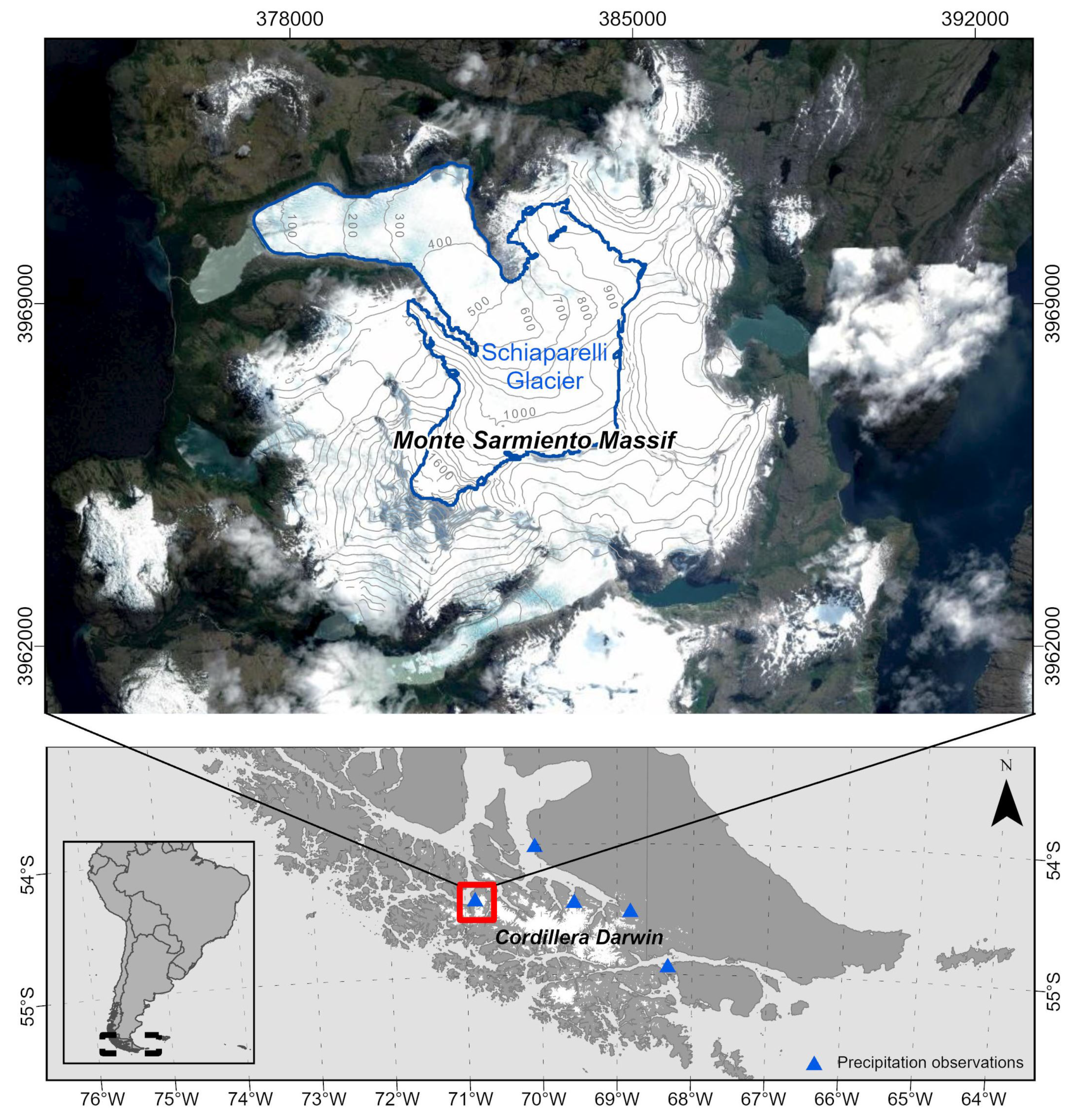
1.2. Study Site

Schiaparelli Glacier descends north-west from Monte Sarmiento (54.39$°$ S to 54.45$°$ S, 70.90$°$ W to 70.77$°$ W), at the southwestern tip of Isla Grande de Tierra del Fuego (Figure 1). The glacier calves into a moraine-dammed proglacial lake which formed after glacier recession in the 1940s [7]. Schiaparelli Glacier underwent late Little Ice Age advances [7]. The existence of three terminal moraine ridges at Schiaparelli Glacier implies a glacial recession without distinct readvances since 1749 ± 5 CE [7]. This year reflects the maximum date of the first moraine stabilization. The oldest deposition of the middle moraine and the one closest to the recent glacier front were dated to 1789 ± 5 CE and 1867 ± 5 CE [7]. The glaciated parts of the Monte Sarmiento Massif have shrunk from 199.3 km${}^2$ in 1870 to 183.1 km${}^2$ in 2011 [14], in particular, due to the shrinkage of the land-terminating glaciers. Area loss was accelerated between 1986 and 2001 [14] while it slowed down after 2001. At Schiaparelli Glacier, an area loss of about 7.5 km${}^2$ from 31.8 km${}^2$ in ∼1870 to 24.3 km${}^2$ 2016 was determined [2].

2. Materials and Methods

2.1. Meteorological and Glaciological Observations

Two automatic weather stations (AWS) are situated within the study area of the Schiaparelli Glacier (Figure 2). AWS${}_{GLACIER}$ is located on the lower part of the glacier at 54.4$°$ S, 70.87$°$ W at about 140 m a.s.l. (location measured in September 2015). The AWS was installed in March 2013 but had to be reinstalled in June 2015 due to the glacier’s movement and the formation of crevasses close to the station. A second AWS (AWS${}_{ROCK}$) has been installed additionally on rock to minimize measurement inaccuracies and failures. The AWS is located on the southern side of the glacier close to the glacier margin (Figure 2) at 54.4$°$ S, 70.87$°$ W, 92 m a.s.l. Both AWS measure hourly air temperature, relative humidity, incoming solar radiation, wind speed, and wind direction. Surface pressure is measured at AWS${}_{GLACIER}$, while precipitation is measured using an unshielded and unheated tipping-bucket rain gauge at AWS${}_{ROCK}$. For modeling purposes, we use hourly data of air temperature, relative humidity, surface pressure, and wind speed of AWS${}_{GLACIER}$ and incoming solar radiation and precipitation of AWS${}_{ROCK}$.

Precipitation datasets of three weather stations, provided by the Chilean Water Directorate (DGA), and one weather station of Charlie Porter ([24], provided by Eñaut Izagirre Estibaritz via personal communication) are used to validate the spatial distribution of modeled precipitation. The data of the following four weather stations (geographical location, data period) have been chosen: Marinelli Glacier (Charlie Porter) (54.43$°$ S, 69.57$°$ W, 08/2011 to 07/2014), Río Azopardo (DGA) (54.50$°$ S, 68.82$°$ W, 08/2011 to 08/2016), Puerto Navarino (DGA) (54.93$°$ S, 68.32$°$ W, Aug 08/2011 to 02/2017 with short data gaps), Río Cóndor (DGA) (54.00$°$ S, 70.08$°$ W, 01/2012 to 02/2017) (Figure 1).

Ablation on the glacier was measured between September 2015 and April 2017. The reading of the ablation stakes (S1 to S3) has been performed twice a year. A higher temporal resolution of individual ablation measurement (S3) was achieved by means of time-lapse imagery (CAM, Figure 2) between September 2015 and April 2016 at the glacier margin. Therefore, we installed a self-constructed time lapse camera south of the glacier margin which took pictures of the glacier area with one installed ablation stake every two hours. The stake is marked every 1.5 m. From this image time series we can determine the periods in which 1.5 m of melt had occurred, providing higher temporal resolution compared to the manual semi-annual readings of ablation stakes.

Lake water level and temperature have been recorded hourly using a HOBO water level pressure sensor (HYDRO, Figure 2). It was installed close to the glacier outflow at the southwest margin of Lago Azul between April 2016 and March 2017. Data gaps occurred during the first austral winter because the measurement site fell dry due to a unexpectedly low lake level.

2.2. Reanalysis Data

Atmospheric model input datasets for COSIPY and the orographic precipitation model (OPM) [27,31] were derived from the latest large-scale ERA-interim reanalysis product supplied by the European Centre for Medium-Range Weather Forecasts (ECMWF) [32]. COSIPY is forced by downscaled 6-hourly surface incoming solar radiation $S{W}_{in}$ (W m${}^{-2}$) and air temperature $T_{2m}$ ($°$C), surface pressure $p_s$ (hPa) as well as relative humidity $r{H}_{2m}$ (%), cloud cover fraction N, and wind speed $u_{2m}$ (m s${}^{-1}$) at 2 m. Data are derived as the means from four grid points covering the study site (−54.5$°$ S and −54.75$°$ S, 71.25$°$ W, and 70.5$°$ W) for the time period from 1 April 2000 to 31 March 2017. Running the OPM to compute total precipitation requires 6-hourly ERA-interim datasets of horizontal and vertical wind components, air temperature at the 850 and 500 hPa level, relative humidity, geopotential heights, and large-scale precipitation. Time series of wind, precipitation, and relative humidity are taken from the 850 hPa level to describe the large-scale prevailing wind conditions and to calculate the background precipitation and filter constraints within the OPM routine [27]. Atmospheric input data were averaged over four grid points located west along the Cordillera Darwin (54.0$°$ S to 54.75$°$ S, 75$°$ W to 74.25$°$ W) to represent upstream conditions.

2.3. Elevation and Glacier Outline

The digital elevation model (DEM) generated from the Shuttle Radar Topography Mission (SRTM) [33,34] is used as the reference surface elevation in 2000 for COSIPY and OPM runs. COSIPY and OPM runs are carried out with spatial resolutions of 200 m and 1000 m, respectively. Glacier outlines for COSIPY model runs have been obtained from the glacier inventory of [2] for 1870 and for 2016 (Figure 2). According to [2], glacier extent during the LIA was digitized manually using the 1986 glacial extent as the starting point and clearly visible morphological evidence, such as vegetation trimlines or moraine systems. The latter represents the maximum extent of the LIA which does not necessarily represent the end of the LIA (∼1870 AD).

2.4. Surface Energy and Climatic Mass Balance Model

Surface energy fluxes and climatic mass balance are estimated using the open-source surface and energy mass balance model COSIPY [29] which is the updated version of the former coupled snowpack and ice surface energy and mass balance model (COSIMA) [28], with updated physics and optimized computational performance. COSIMA is described in detail in [28] and has been successfully applied for selected glaciers at the Southern Patagonia Icefield [27]. Only a short description of the model physics is therefore provided in the following. COSIPY combines a surface energy balance model with a multi-layer sub-surface snow and ice model to resolve estimated energy fluxes and surface mass balance processes [29]. All energy fluxes F that contribute to the surface energy budget and the energy available for surface melting $Q_{melt}$ [35] are considered in the energy balance model:

$$F=S{W}_{in}·(1-\alpha )+L{W}_{in}+L{W}_{out}+Q_{sens}+Q_{lat}+Q_g.$$

(1)

The model takes into consideration: the incoming shortwave radiation $S{W}_{in}$, the albedo $\alpha$, the incoming $L{W}_{in}$ and outgoing longwave radiation $L{W}_{out}$, the sensible $Q_{sens}$ and latent heat fluxes $Q_{lat}$, and the ground heat flux $Q_g$. Ablation occurs due to sublimation, evaporation, subsurface melt, and surface melt. $Q_{melt}$ requires the surface temperature $T_s$ to be at the melting point (0 $°$C) and a positive energy flux F towards the surface to prevail. In this case, $Q_{melt}$ equals F. Each layer is characterized by a temperature, density, and liquid water content. Turbulent heat fluxes $Q_{sens}$ and $Q_{lat}$, are calculated based on the the bulk aerodynamic method [35] between the surface and two meters above ground by means of $T_{2m}$, $r{H}_{2m}$, and $u_{2m}$. $Q_g$ consists of fluxes of heat conduction and penetrating shortwave radiation [28]. Detailed information about the parameter settings in COSIPY, e.g., model domain, layer depth, and albedo values, can be found in

Table 1. COSIPY and OPM parameter settings based on findings from [27]. Values denoted with * are mean values.

	Parameter	Value/Range	Unit	Fixed/Calculated	Source
COSIPY	Total domain depth	100	m	F	-
	Model layer thickness	0.1	m	F	-
	Ice albedo	0.3	-	F	[36]
	Fresh snow albedo	0.9	-	F	[28]
	Firn albedo	0.45	-	F	[36]
	Initial subsurface temperature	273.15	$°$C	F	[27]
	Air temperature lapse rates	−0.67, −0.73	$°$C 100 m${}^{-1}$	F	[27]
	Surface pressure gradient	−0.105	hPa m${}^{-1}$	F	[27]
	Snow density for $P_{solid}$	250	kg m${}^{-3}$	F	[28]
	Threshold for $P_{solid}$ to $P_{liq}$	0–2.0	$°$C	F	[37]
	Snow pack density profile	250 to 550	kg m${}^{-3}$	C	[28]
OPM	Uplift sensitivity factor	0.006 *	-	C	[38]
	Water vapor scale height	2382 *	m	C	[38]
	Conversion/fallout time scale	1824 *	m s${}^{-1}$	C	[39]
	Brunt-Väisälä frequency	0.009 *	s${}^{-1}$	C	[38]
	Averaged falling speed	1.3	m s${}^{-1}$	F	[27]
	Thresholds relative humidity	80, 85, 90	%	F	[38]

.

2.4.1. Climate Forcing of COSIPY

COSIPY is driven by surface incoming solar radiation $S{W}_{in}$ (W m${}^{-2}$), air temperature $T_{2m}$ ($°$C), relative humidity $r{H}_{2m}$ (%), surface pressure $p_s$ (hPa), wind speed at 2 m $u_{2m}$ (m s${}^{-1}$), cloud cover fraction N, and total precipitation $RRR$. We use different approaches to downscale ERA-interim data of $T_{2m}$, $r{H}_{2m}$, $p_s$, $S{W}_{in}$, and total precipitation $RRR$ by means of observed data which are described in more detail in [27].

Precipitation fields are modeled using an analytical OPM based on the linear steady-state theory of airflow dynamics [38,40]. A more detailed description and validation of the model itself is given by [38] and [40] while the methodical application as used in this study is described in more detail in [27,31]. The OPM estimates $RRR$ resulting from the forced orographic uplift of air masses over a mountain assuming stable and saturated atmospheric conditions. The model estimates the condensation rate by the terrain-induced vertical air velocity, and the horizontal wind speed and advection of water vapor, and includes effects of airflow dynamics and downslope evaporation as well. The main term of the linear model describing the orographic precipitation ($P_{oro}$) generation is solved in Fourier space for each Fourier component (k,l) as follows.

$${\widehat{P}}_{oro}(k,l)=\frac{C_w·i·\sigma ·\widehat{h}(k,l)}{(1-i·m·H_w)(1+i·\sigma ·{\tau }_c)(1+i·\sigma ·{\tau }_f)}.$$

(2)

Equation (2) includes an uplift sensitivity factor $C_{\mathrm{w}}$, the water vapor scale height $H_{\mathrm{w}}$, the complex number i, the intrinsic frequency $\sigma$, the Fourier transform of the orography $\widehat{h}$, the vertical wavenumber m, and the delay time scales for conversion ${\tau }_{\mathrm{c}}$ and fallout ${\tau }_{\mathrm{f}}$ of hydrometeors. The thermodynamic sensitivity $C_{\mathrm{w}}$ accounts for the effects of saturation water vapor density, and the moist adiabatic and environmental lapse rates. $H_{\mathrm{w}}$ mainly depends on the environmental air temperature and lapse rate. Airflow dynamics are represented by the intrinsic frequency, including the vertical and horizontal winds. One of the airflow features included is the decay of vertical velocity with altitude which is described by m. The calculation of m contains the buoyancy frequency in a saturated atmosphere and the moist Brunt-Väisälä frequency $N_{\mathrm{m}}$ to consider the effect of moist air masses on the static stability. Additionally, the precipitation generation is shifted downstream from the water source region depending on the wind speed and the cloud time parameters ${\tau }_c$ and ${\tau }_f$. The total amount of precipitation $RRR$ is assessed by considering the large-scale precipitation which in this study is derived from ERA-interim precipitation data. For detailed information about the procedure and the parameter settings, the reader is referred to [27] and Table 1. The amount of solid precipitation is determined in COSIPY by applying a hyperbolic tangent function [27,37] to the modeled OPM precipitation fields. The proportion of solid precipitation to total precipitation is smoothly scaled between 100% and 0% within a $T_{2m}$ range of 0 $°$C and 2 $°$C [27,37]. The temperature range of the transition from liquid to solid is similar to the assumptions used by [36,41] to determine the solid precipitation fraction.

OPM runs have been carried out with varying thresholds of the model constraint $rH$ according to the values used in previous studies (e.g., [27,42,43,44]) to find the best model fit compared to observed data. OPM runs were calibrated with observed data from AWS${}_{ROCK}$ between October 2015 to September 2016. Best-fits have been achieved using the constraint $rH$≥ 85. Best-fit OPM results were compared to observed precipitation data of five weather stations (Figure 3A). The explained variance between modeled and observed monthly precipitation data was 93% for ROCK, 74% for AZO, 71% for MAR, 43% for NAV, and 44% for CON. The amount of modeled orographic precipitation of the total modeled precipitation amount is highest for AWS${}_{ROCK}$ with 43%. The AWS is located at the western side of the Monte Sarmiento Massif and therefore strongly influenced by orographic effects. OPM results for the other weather stations were mainly determined by the downscaling results of ERA-interim precipitation, because their locations are less influenced by orographic effects. The glacier-wide mean of $RRR$ averaged over the study period 2000 to 2017 is 4.0 m w.e. a${}^{-1}$ with a maximal amount of 5.6 ± 0.5 m w.e. a${}^{-1}$ in the upper part of the glacier. The glacier-wide amount of solid precipitation to total precipitation is about 38 %.

$T_{2m}$, $r{H}_{2m}$, and $p_s$ were statistically downscaled from ERA-interim data to AWS${}_{GLACIER}$ by using quantile mapping (e.g., [45,46]). Bias-corrected air temperature and surface pressure were spatially interpolated using a fixed lapse rates from the AWS location (Table 1). Downscaling results of daily ERA-interim $T_{2m}$ by means of station data are visualized in Figure 3B. For the validation period, the chosen downscaling method tends to overestimate low temperatures while high temperatures are slightly underestimated. The glacier-wide mean $T_{2m}$ averaged between 2000 and 2017 is 0.6 ± 0.3 $°$C.

Incoming shortwave radiation $S{W}_{in}$ was also downscaled from ERA-interim data to the measured solar radiation at AWS${}_{ROCK}$ using quantile mapping. The spatial distribution of $S{W}_{in}$ was then derived from a modified radiation model according to [47] that computes clear-sky direct and diffuse shortwave radiation depending on the geographical position, elevation, albedo, and shading by the surrounding terrain, and the slope and aspect over the glacier domain. At each time step and grid cell, the potential clear-sky radiation is corrected for cloud cover by means of downscaled $S{W}_{in}$. Therefore, we calculate the ratio between potential clear-sky radiation at AWS${}_{ROCK}$ and any other pixel within the glacier domain. $S{W}_{in}$ at each pixel is then derived by multiplying the calculated ratio and the downscaled $S{W}_{in}$ at AWS${}_{ROCK}$. The glacier-wide mean $S{W}_{in}$ averaged between 2000 and 2017 is +91 W m${}^{-2}$.

2.4.2. Uncertainty Assessment of COSIPY and OPM

Ablation stake measurements carried out at Schiaparelli Glacier between 2015 and 2017 were used to validate the modeled climatic mass balance. We forced COSIPY once with observed timeseries. In this case only N was taken from ERA-interim and used to calculate longwave incoming radiation. Secondly, we ran COSIPY with downscaled ERA-interim data. The RMSE between model ran and observed values were ± 0.67 m w.e. for the AWS run and ± 0.71 m w.e. for the ERA-interim run between October 2015 and March 2017. COSIPY driven by both observed and downscaled input data reproduces measured ablation well (Figure 4). The uncertainties of modeled climatic mass balance were estimated by accounting for uncertainties in the spatial distributions of input datasets of air temperature and solid precipitation due to the lack of observations in the accumulation area. The spatial distribution of air temperature is determined by the chosen lapse rate, while the amount of modeled precipitation is mainly controlled by the OPM filter constraint $rH$ which regulates the amount of orographic induced precipitation to large-scale precipitation within the OPM [27]. We therefore include varying values of air temperature lapse rate and the OPM filter constraint $rH$ for the assessment of climatic mass balance uncertainties. In total, six runs were carried out for the mass balance years 2015/16 and 2016/17 to assess the uncertainty of glacier-wide climatic mass balance. As lower and upper air temperature lapse rates, we assumed 0.67 $°$C and 0.73 $°$C 100 m${}^{-1}$ as used in earlier mass balance studies (e.g., [27]). Thresholds of 80%, 85%, and 90% for $rH$ were considered. The standard deviation between those six different model runs was ± 0.36 m w.e. Best-fit simulation results were achieved using 0.67 $°$C and running the OPM with a $rH$ threshold of 85%.

2.5. Little Ice Age Estimations

We followed the approach of [48] to reconstruct LIA climate by assuming that the glacier was in equilibrium over a short period of time during the formation of the associated terminal moraines when climate started to shift from LIA to present-day climate conditions. First, we simulated the climatic conditions which were needed to derive steady-state conditions for the recent extent of Schiaparelli Glacier. Therefore, precipitation and air temperature offsets to the present-day climate were used as COSIPY forcing to derive an average CMB in equilibrium. We chose the time period 2000 to 2010 as the simulation period. LIA climate was then reconstructed, using precipitation and air temperature offsets along with the LIA glacier extent [49] and adapted glacier height by means of SRTM data and moraine system information. All other input parameters of COSIPY as well as the altitudinal gradients remained unchanged. Glacier height during the LIA was reconstructed by using glacier outline information from 2000 and LIA as well as SRTM data with a resolution of 200 m (Figure 5). First, we compared vegetation trimline and moraine information [7] with SRTM heights extracted at the LIA outline of the glacier. We then calculated height differences ($h_{dif}$) for each pixel between the glacier outline of 2000 and LIA (Figure 5A). We then manually digitized the glacier flowline based on the center of elevation contours (contour lines of 50 m). The maximum height difference along the LIA outlines ($h_{dif,max}$) perpendicular to any position along the flowline was added to the height (h) of the pixel at this position of the flowline (Figure 5A). Finally, we linearly interpolated between the heights at the glacier’s LIA outlines and the height adjusted flowline (Figure 5A). This procedure was limited to the part of the glacier where the LIA glacier outline extends further than the glacier outline in 2000 (Figure 5A, inset). The resulting height changes are visualized in Figure 5B. For Schiaparelli Glacier, this area approximately coincides with the area below the ELA. The heights of the upper parts were left unchanged. For LIA climate reconstruction, COSIPY was driven using the DEM adapted to LIA conditions. We further used COSIPY runs based on the initial SRTM heights for comparison and uncertainty assessment. The standard deviation between all runs is ± 0.12 m w.e.

3. Results and Discussion

The evaluations of COSIPY-modeled surface energy fluxes and climatic mass balance are discussed in the following.

The glacier-wide mean annual surface energy balance and climatic mass balance components are shown in Figure 6A,B. The glacier-wide energy input is dominated year-around by $L{W}_{in}$ (+292 W m${}^{-2}$) and $S{W}_{in}$ (+91 W m${}^{-2}$), followed by $Q_{sens}$ (+32 W m${}^{-2}$). Available energy at the glacier surface is consumed by $L{W}_{out}$ (−296 W m${}^{-2}$), $S{W}_{out}$ (−65 W m${}^{-2}$), $Q_{lat}$ (−9 W m${}^{-2}$), $Q_g$ (−1 W m${}^{-2}$), and $Q_{melt}$ (−44 W m${}^{-2}$). The modeled glacier-wide mean annual CMB for Schiaparelli Glacier is estimated to −1.8 ± 0.36 m w.e. a${}^{-1}$ averaged between April 2000 and March 2017. The CMB is negative for each year during the complete study period (Figure 6B). Glacier melt was highest during the mass balance year 2016/17, followed by the mass balance years between 2003/04 and 2006/07. The highest CMB of −0.7 ± 0.36 m w.e. a${}^{-1}$ is modeled for the mass balance year 2009/10 which coincides with above-average $P_{solid}$ amounts and lower $T_{2m}$ values (Figure 7A). Mean annual $T_{2m}$ values which are above the average as in the mass balance years 2007/08 and 2008/09 cause high negative CMB values and cannot be fully compensated by positive $P_{solid}$ amounts or low $S{W}_{in}$ values. In general, the climatic mass balance is dominated by surface melt (60%) and solid precipitation (37%). Sublimation, deposition, refreezing, and evaporation play only minor roles. Strong correlations between CMB and $T_{2m}$ (r = −0.77) and CMB and $P_{solid}$ (r = 0.80) reflect this finding (Figure 7B). However, we cannot find any meaningful correlation between CMB and $S{W}_{in}$. Modeled annual ELA ranges from 650 ± 50 m a.s.l. to 800 ± 50 m a.s.l. with a mean of 730 ± 50 m a.s.l. These ranges are similar to values in [4].

In a previous study of [27], CMB simulations using the former version of COSIPY were carried out at the two lake-terminating glaciers Grey and Tyndall located at the eastern side of the SPI (

Table 2. Comparison of glacier characteristics and COSIPY/COSIMA results between the glaciers Grey (SPI), Tyndall (SPI), and Schiaparelli (MSM), averaged over the period 2000–2016. Listed are glacier size (km${}^2$) and modeled annual glacier-wide mean CMB, ELA, P${}_{solid}$, T${}_{2m}$, SW${}_{net}$, LW${}_{net}$, Q${}_{sens}$, and Q${}_{lat}$.

Glacier	Size km${}^2$	CMB m w.e.	ELAm a.s.l	P${}_{\mathit{solid}}$ m w.e.	T${}_{2\mathit{m}}$ $°$C	SW${}_{\mathit{net}}$ W m${}^{-2}$	LW${}_{\mathit{net}}$ W m${}^{-2}$	Q${}_{\mathit{sens}}$ W m${}^{-2}$	Q${}_{\mathit{lat}}$ W m${}^{-2}$
Grey	239	+0.86 ± 0.52	960 ± 70	5.9 ± 1.0	−2.4 ± 0.6	39	−9	11	−9
Tyndall	301	+0.41 ± 0.54	920 ± 60	7.1 ± 1.1	−0.7 ± 0.5	45	−18	16	−7
Schiaparelli	24	−1.69 ± 0.36	730 ± 50	2.3 ± 0.3	0.6 ± 0.3	26	−5	32	−10

). Climate conditions at Grey Glacier and Tyndall Glacier are wetter and colder compared to Schiaparelli Glacier as a result of higher altitudes in general and the stronger influence of orographic effects on precipitation distribution (e.g., [27,50]). Comparing the energy balance components, it is striking that the shortwave net radiation is much lower at the MSM than at the SPI while the sensible heat flux is more important as a source of energy input at the glacial surface. All three glaciers underwent a massive retreat in the past decade. However, climatic mass balance simulations are positive with a glacier-wide mean annual of +0.86 ± 0.52 m w.e. a${}^{-1}$ for Grey Glacier and +0.41 ± 0.54 m w.e. a${}^{-1}$ for Tyndall Glacier between 2000 and 2016, while the CMB of Schiaparelli Glacier is clearly negative with −1.69 ± 0.36 m w.e. a${}^{-1}$. The positive CMB of Grey Glacier and Tyndall Glacier cannot fully compensate the mass loss which is caused by dynamical ice processes, especially calving into the lakes and frontal ablation. Remote sensing studies of [3,23] do not show extensive glacier thinning at Schiaparelli Glacier. Therefore, we conclude that mass loss due to surface mass balance processes seems to be the main reason for the recent areal changes of Schiaparelli Glacier. This is in accordance with several other studies [24,51] that suggest that the recent mass loss of most glaciers at the CDI and surrounding icefields is rather driven by atmospheric warming than by dynamical ice processes such as calving, except for a few calving glaciers, such as Marinelli, which has experienced a remarkable retreat of more than 10 km between 1945 and 2000 [52].

3.1. Link between Climatic Mass Balance and Lake Level Changes

We compare meteorological data and modeled climatic glacier mass balance with lake level height changes at Lago Azul on a daily basis for a short measurement period during the austral summer 2016/2017 (Figure 8). Relating daily air temperature to the height of the lake level showed the highest correlation r = 0.6 using a time lag of +1 day (d + 1) (Figure 8A). Lower correlations were calculated for larger time lags. There was no pronounced link between the other meteorological observations and lake level changes; in particular, we could not obtain any meaningful correlation between precipitation and lake level (Figure 8B).

The correlation between CMB, averaged over the area beneath the mean modeled ELA, and lake level height changes is r = 0.40 at d + 1 (Figure 8C). Information on frontal ablation and lake bathymetry will allow a more extensive analysis of the link between glacier runoff and changes in lake level height and outflow in the future.

3.2. Reconstruction of LIA Climate

The reconstruction of steady state climate conditions during LIA requires as starting point a glacier in equilibrium under present-day climate conditions. We therefore, first simulate the climatic conditions which are needed to derive steady-state conditions for the recent extent of Schiaparelli Glacier. Several temperature (TO) and precipitation offset (PO) combinations lead to a zero CMB of Schiaparelli Glacier based on the recent extent (

Table 3. Precipitation (PO) and air temperature offsets (TO) are combined to simulate steady-state conditions (m w.e. a${}^{-1}$) for the recent extent of Schiaparelli Glacier.

TO/PO	−10%	−5%	0%	5%	10%	15%	20%	25%	30%
0.0 $°$C			−1.81
−0.4 $°$C								−0.29	−0.17
−0.5 $°$C							−0.22	−0.08	0.05
−0.6 $°$C						−0.14	−0.01	0.13
−0.7 $°$C					−0.07	0.06	0.20
−0.8 $°$C			−0.16	−0.02	0.12
−0.9 $°$C		−0.13	0.02
−1.0 $°$C	−0.10	0.05	0.19

). An air temperature decrease between −0.5 $°$C and −0.9 $°$C in combination with a precipitation increase of up to 30% seems to be realistic. A zero CMB under actual climate conditions between 2000 and 2010 would imply a glacier length reduction of about 3.8 km back from the glacier front in 2016. Precipitation and air temperature offsets to the present-day climate are used as COSIPY forcing to derive an average CMB in equilibrium. We choose the combination TO = −0.6 $°$C and PO = 20% for representing the recent steady-state climate conditions. LIA climate is then reconstructed, using precipitation and air temperature offsets along with the LIA glacier extent [2] and the adapted glacier height. Forcing COSIPY with the recent steady-state climate conditions, the CMB of Schiaparelli Glacier in 1870 is negative with −1.64 ± 0.48 m w.e. a${}^{-1}$. A nearly zero CMB is simulated by forcing the model with air temperature offsets between −0.4 and −0.8 $°$C in combination with an increase in precipitation of up to 30% to the artificial steady-state of 2000–2010 (

Table 4. Precipitation (PO) and air temperature offsets (TO) are combined to simulate steady-state conditions (m w.e. a${}^{-1}$) for the LIA extent of Schiaparelli Glacier based on the adapted SRTM heights.

TO/PO	−10%	−5%	0%	5%	10%	15%	20%	25%	30%
0.0 $°$C			−1.64
−0.4 $°$C							−0.23	−0.09	0.05
−0.5 $°$C						−0.17	−0.02	0.12
−0.6 $°$C					−0.13	0.03
−0.7 $°$C				−0.08	0.07
−0.8 $°$C			−0.03	0.12
−0.9 $°$C	−0.13	0.01	0.17
−1.0 $°$C	0.05	0.19	0.34

). The higher the air temperature offset, the smaller the precipitation offset. Previous studies about Holocene climate reconstruction in Southern Patagonia [53,54,55] indicate colder and wetter conditions during the LIA. According to [4] temperature anomalies differed regionally; the mean air temperature was below the 1900–1990 means by 0.86 $°$C in the southern parts of Southern Andes. For Schiaparelli Glacier, we obtained with respect to the actual climate in 2000–2010, a combined lowering of air temperature between −0.9 $°$C and −1.7 $°$C, a precipitation increase of up to +60% by summing up the offsets for steady state conditions in 2000–2010, and the further adjustment of climate to allow LIA steady-state conditions of CMB.

4. Conclusions

The surface energy and mass balance model COSIPY was applied to simulate the climatic mass balance of Schiaparelli Glacier between 2000 and 2017 and during the LIA (1870). A glacier-wide mean annual climatic mass balance of −1.8 ± 0.36 m w.e. a${}^{-1}$ was simulated between between April 2000 and March 2017. A lowest negative CMB of −0.7 ± 0.36 m w.e. a${}^{-1}$ was modeled for the mass balance year 2009/10 as the result from the above-average $P_{solid}$ amounts and lower $T_{2m}$ values compared to the mean between 2000 and 2017. Incoming solar radiation and the sensible heat flux are the main sources of energy input at the glacial surface. The contributions of subsurface melt, sublimation, refreezing, and evaporation are comparatively small. Observed air temperature and modeled climatic mass balance can be linked to changes in lake level heights at Lago Azul. Frontal ablation and calving seem to play a minor role in the mass balance of Schiaparelli Glacier when compared to other larger glaciers in CDI and SPI. An extended record of lake level from on-going measurements combined with runoff measurements at the outlet from the lake to the sea will allow a more detailed assessment of the glacial hydrology at Schiaparelli glacier in future studies. We assumed a zero CMB at the turning point of Schiaparelli Glacier from being in equilibrium in 1870 to retreating until now. Assuming recent steady-state climate conditions, the CMB of Schiaparelli Glacier in 1870 would have been significantly negative with −1.64 ± 0.48 m w.e. a${}^{-1}$. A nearly zero CMB was simulated by forcing COSIPY with air temperature offsets between −0.4 to −0.8 $°$C in combination with an increase in precipitation of up to +30% to the present-day steady state climate conditions. The upper limit of air temperature decrease is similar to previous studies about Holocene climate reconstruction in Southern Patagonian [53,54,55] which also indicate colder and wetter conditions during the LIA. The lack of observed accumulation data causes high uncertainties in surface mass balance simulations regarding the glacier-wide amount of solid precipitation. Missing information about the bedrock topography or ice thickness limited the applicability of dynamical ice models up to now. Future studies incorporating ice-dynamical modeling will allow one to quantify ice’s dynamical processes and their impact on the overall mass loss compared to the climatic mass balance forcing.

References

- Lopez, P.; Chevallier, P.; Favier, V.; Pouyaud, B.; Ordenes, F.; Oerlemans, J. A regional view of fluctuations in glacier length in southern South America. Glob. Planet. Chang. 2010, 71, 85–108. [Google Scholar] [CrossRef]
- Meier, W.J.H.; Grießinger, J.; Hochreuther, P.; Braun, M.H. An Updated Multi-Temporal Glacier Inventory for the Patagonian Andes With Changes Between the Little Ice Age and 2016. Front. Earth Sci. 2018, 6, 62. [Google Scholar] [CrossRef] [Green Version]
- Melkonian, A.K.; Willis, M.J.; Pritchard, M.E.; Rivera, A.; Bown, F.; Bernstein, S.A. Satellite-derived volume loss rates and glacier speeds for the Cordillera Darwin Icefield, Chile. Cryosphere 2013, 7, 823–839. [Google Scholar] [CrossRef] [Green Version]
- Strelin, J.; Casassa, G.; Rosqvist, G.; Holmlund, P. Holocene glaciations in the Ema Glacier Valley, Monte Sarmiento Massif, Tierra del Fuego. Palaeogeogr. Palaeoclimatol. Palaeoecol. 2008, 260, 299–314. [Google Scholar] [CrossRef]
- Masiokas, M.H.; Rivera, A.; Espizua, L.E.; Villalba, R.; Delgado, S.; Aravena, J.C. Glacier fluctuations in extratropical South America during the past 1000 years. Palaeogeogr. Palaeoclimatol. Palaeoecol. 2009, 281, 242–268. [Google Scholar] [CrossRef]
- Koch, J. Little Ice Age and recent glacier advances in the Cordillera Darwin, Tierra del Fuego, Chile. Anales Instituto Patagonia (Chile) 2015, 43, 127–136. [Google Scholar] [CrossRef] [Green Version]
- Meier, W.J.H.; Aravena, J.C.; Grießinger, J.; Hochreuther, P.; Soto-Rogel, P.; Zhu, H.; Pol-Holz, R.D.; Schneider, C.; Braun, M.H. Late Holocene Glacial Fluctuations of Schiaparelli Glacier at Monte Sarmiento Massif, Tierra del Fuego (54°24′ S). Geosciences 2019, 9, 340. [Google Scholar] [CrossRef] [Green Version]
- Koch, J.; Kilian, R. ‘Little Ice Age’ glacier fluctuations, Gran Campo Nevado, southernmost Chile. Holocene 2005, 15, 20–28. [Google Scholar] [CrossRef]
- Aniya, M. Holocene glaciations of Hielo Patagacico (Patagonia Icefield), South America: A brief review. Geochem. J. 2013, 47, 97–105. [Google Scholar] [CrossRef] [Green Version]
- Glasser, N.F.; Harrison, S.; Winchester, V.; Aniya, M. Late Pleistocene and Holocene palaeoclimate and glacier fluctuations in Patagonia. Glob. Planet. Chang. 2004, 43, 79–101. [Google Scholar] [CrossRef]
- Kilian, R.; Lamy, F. A review of Glacial and Holocene paleoclimate records from southernmost Patagonia (49–55 °S). Quat. Sci. Rev. 2012, 53, 1–23. [Google Scholar] [CrossRef]
- Villalba, R.; Lara, A.; Boninsegna, J.A.; Masiokas, M.; Delgado, S.; Aravena, J.C.; Roig, F.A.; Schmelter, A.; Wolodarsky, A.; Ripalta, A. Large-Scale Temperature Changes Across the Southern Andes: 20th-Century Variations in the Context of the Past 400 Years. In Climate Variability and Change in High Elevation Regions: Past, Present & Future; Diaz, H.F., Ed.; Springer: Dordrecht, The Netherlands, 2003; pp. 177–232. [Google Scholar] [CrossRef]
- Rosenblüth, B.; Fuenzalida, H.A.; Aceituno, P. Recent temperature variations in southern South America. Int. J. Climatol. 1997, 17, 67–85. [Google Scholar] [CrossRef]
- Davies, B.; Glasser, N. Accelerating shrinkage of Patagonian glaciers from the Little Ice Age (AD 1870) to 2011. J. Glaciol. 2012, 58, 1063–1084. [Google Scholar] [CrossRef] [Green Version]
- Holmlund, P.; Fuenzalida, H. Anomalous glacier responses to 20th century climatic changes in Darwin Cordillera, southern Chile. J. Glaciol. 1995, 41, 465–473. [Google Scholar] [CrossRef] [Green Version]
- Aniya, M.; Sato, H.; Naruse, R.; Skvarca, P.; Casassa, G. The use of satellite and airborne imagery to inventory outlet glaciers of the southern Patagonia Icefield, South America. Photogramm. Eng. Remote Sens. 1996, 62, 1361–1369. [Google Scholar]
- Rivera, A.; Casassa, G. Volume changes on Pío XI glacier, Patagonia: 1975–1995. Glob. Planet. Chang. 1999, 22, 233–244. [Google Scholar] [CrossRef]
- Rivera, A.; Benham, T.; Casassa, G.; Bamber, J.; Dowdeswell, J.A. Ice elevation and areal changes of glaciers from the Northern Patagonia Icefield, Chile. Glob. Planet. Chang. 2007, 59, 126–137. [Google Scholar] [CrossRef]
- Willis, M.J.; Melkonian, A.K.; Pritchard, M.E.; Ramage, J.M. Ice loss rates at the Northern Patagonian Icefield derived using a decade of satellite remote sensing. Remote Sens. Environ. 2012, 117, 184–198. [Google Scholar] [CrossRef]
- Sakakibara, D.; Sugiyama, S. Ice-front variations and speed changes of calving glaciers in the Southern Patagonia Icefield from 1984 to 2011. J. Geophys. Res. Earth Surf. 2014, 119, 2541–2554. [Google Scholar] [CrossRef]
- Minowa, M.; Sugiyama, S.; Sakakibara, D.; Sawagaki, T. Contrasting glacier variations of Glaciar Perito Moreno and Glaciar Ameghino, Southern Patagonia Icefield. Ann. Glaciol. 2015, 56, 26–32. [Google Scholar] [CrossRef] [Green Version]
- Malz, P.; Meier, W.; Casassa, G.; Jaña, R.; Skvarca, P.; Braun, M.H. Elevation and Mass Changes of the Southern Patagonia Icefield Derived from TanDEM-X and SRTM Data. Remote Sens. 2018, 10, 188. [Google Scholar] [CrossRef] [Green Version]
- Braun, M.H.; Malz, P.; Sommer, C.; Farías-Barahona, D.; Sauter, T.; Casassa, G.; Soruco, A.; Skvarca, P.; Seehaus, T.C. Constraining glacier elevation and mass changes in South America. Nat. Clim. Chang. 2019, 9, 130–136. [Google Scholar] [CrossRef]
- Koppes, M.; Hallet, B.; Anderson, J. Synchronous acceleration of ice loss and glacial erosion, Glaciar Marinelli, Chilean Tierra del Fuego. J. Glaciol. 2009, 55, 207–220. [Google Scholar] [CrossRef] [Green Version]
- Dussaillant, I.; Berthier, E.; Brun, F.; Masiokas, M.; Hugonnet, R.; Favier, V.; Rabatel, A.; Pitte, P.; Ruiz, L. Two decades of glacier mass loss along the Andes. Nat. Geosci. 2019, 12, 802–808. [Google Scholar] [CrossRef]
- Masiokas, M.H.; Rabatel, A.; Rivera, A.; Ruiz, L.; Pitte, P.; Ceballos, J.L.; Barcaza, G.; Soruco, A.; Bown, F.; Berthier, E.; et al. A Review of the Current State and Recent Changes of the Andean Cryosphere. Front. Earth Sci. 2020, 8, 99. [Google Scholar] [CrossRef]
- Weidemann, S.S.; Sauter, T.; Malz, P.; Jaña, R.; Arigony-Neto, J.; Casassa, G.; Schneider, C. Glacier Mass Changes of Lake-Terminating Grey and Tyndall Glaciers at the Southern Patagonia Icefield Derived From Geodetic Observations and Energy and Mass Balance Modeling. Front. Earth Sci. 2018, 6, 81. [Google Scholar] [CrossRef] [Green Version]
- Huintjes, E.; Sauter, T.; Schröter, B.; Maussion, F.; Yang, W.; Kropáček, J.; Buchroithner, M.; Scherer, D.; Kang, S.; Schneider, C. Evaluation of a Coupled Snow and Energy Balance Model for Zhadang Glacier, Tibetan Plateau, Using Glaciological Measurements and Time-Lapse Photography. Arctic Antarctic Alpine Res. 2015, 47, 573–590. [Google Scholar] [CrossRef]
- Sauter, T.; Arndt, A.; Schneider, C. COSIPY v1.2–An open-source coupled snowpack and ice surface energy and mass balance model. Geosci. Model Dev. Discuss. 2020, 2020, 1–25. [Google Scholar] [CrossRef]
- Consortium, R. Randolph Glacier Inventory—A Dataset of Global Glacier Outlines: Version 5.0.: Technical Report. In Global Land Ice Measurements from Space; Digital Media: Boulder, CO, USA, 2015. [Google Scholar] [CrossRef]
- Weidemann, S.; Sauter, T.; Schneider, L.; Schneider, C. Impact of two conceptual precipitation downscaling schemes on mass-balance modeling of Gran Campo Nevado ice cap, Patagonia. J. Glaciol. 2013, 59, 1106–1116. [Google Scholar] [CrossRef] [Green Version]
- Dee, D.; Uppala, S.; Simmons, A.; Berrisford, P.; Poli, P.; Kobayashi, S.; Andrae, U.; Balmaseda, M.; Balsamo, G.; Bauer, P.; et al. The ERA-Interim reanalysis: Configuration and performance of the data assimilation system. Q. J. R. Meteorol. Soc. 2011, 137, 553–597. [Google Scholar] [CrossRef]
- Hoffmann, J.; Walter, D. How Complementary are SRTM-X and-C Band Digital Elevation Models? Photogramm. Eng. Remote Sens. 2006, 72, 261–268. [Google Scholar] [CrossRef] [Green Version]
- Jarvis, A.; Reuter, H.; Nelson, A.; Guevara, E. Hole-Filled Seamless SRTM data V4; International Centre for Tropical Agriculture (CIAT): Cali, Colombia, 2008. [Google Scholar]
- Oerlemans, J. Glaciers and Climate Change; Swets and Zeitlinger: Lisse, The Netherland, 2001. [Google Scholar]
- Schaefer, M.; Machguth, H.; Falvey, M.; Casassa, G.; Rignot, E. Quantifying mass balance processes on the Southern Patagonia Icefield. Cryosphere 2015, 9, 25–35. [Google Scholar] [CrossRef] [Green Version]
- Möller, M.; Schneider, C.; Kilian, R. Glacier change and climate forcing in recent decades at Gran Campo Nevado, southernmost Patagonia. Ann. Glaciol. 2007, 46, 136–144. [Google Scholar] [CrossRef] [Green Version]
- Smith, R.B.; Barstad, I. A Linear Theory of Orographic Precipitation. J. Atmos. Sci. 2004, 61, 1377–1391. [Google Scholar] [CrossRef]
- Jiang, Q.; Smith, R.B. Cloud Timescales and Orographic Precipitation. J. Atmos. Sci. 2003, 60, 1543–1559. [Google Scholar] [CrossRef]
- Barstad, I.; Smith, R.B. Evaluation of an Orographic Precipitation Model. J. Hydrometeorol. 2005, 6, 85–99. [Google Scholar] [CrossRef]
- Aguirre, F.; Carrasco, J.; Sauter, T.; Schneider, C.; Gaete, K.; Garín, E.; Adaros, R.; Butorovic, N.; Jaña, R.; Casassa, G. Snow Cover Change as a Climate Indicator in Brunswick Peninsula, Patagonia. Front. Earth Sci. 2018, 6, 130. [Google Scholar] [CrossRef]
- Crochet, P.; Jóhannesson, T.; Jónsson, T.; Sigurðsson, O.; Björnsson, H.; Pálsson, F.; Barstad, I. Estimating the Spatial Distribution of Precipitation in Iceland Using a Linear Model of Orographic Precipitation. J. Hydrometeorol. 2007, 8, 1285–1306. [Google Scholar] [CrossRef]
- Schuler, T.V.; Crochet, P.; Hock, R.; Jackson, M.; Barstad, I.; Jóhannesson, T. Distribution of snow accumulation on the Svartisen ice cap, Norway, assessed by a model of orographic precipitation. Hydrol. Process. 2008, 22, 3998–4008. [Google Scholar] [CrossRef]
- Jarosch, A.H.; Anslow, F.S.; Clarke, G.K.C. High-resolution precipitation and temperature downscaling for glacier models. Clim. Dyn. 2012, 38, 391–409. [Google Scholar] [CrossRef]
- Panofsky, H.; Brier, G. Some Applications of Statistics to Meteorology; Earth and Mineral Sciences Continuing Education, College of Earth and Mineral Sciences: University Park, PA, USA, 1968. [Google Scholar]
- Gudmundsson, L.; Bremnes, J.B.; Haugen, J.E.; Engen-Skaugen, T. Technical Note: Downscaling RCM precipitation to the station scale using statistical transformations—A comparison of methods. Hydrol. Earth Syst. Sci. 2012, 16, 3383–3390. [Google Scholar] [CrossRef] [Green Version]
- Kumar, L.; Skidmore, A.K.; Knowles, E. Modelling topographic variation in solar radiation in a GIS environment. Int. J. Geogr. Inf. Sci. 1997, 11, 475–497. [Google Scholar] [CrossRef]
- Huintjes, E.; Loibl, D.; Lehmkuhl, F.; Schneider, C. A modelling approach to reconstruct Little Ice Age climate from remote-sensing glacier observations in southeastern Tibet. Ann. Glaciol. 2016, 57, 359–370. [Google Scholar] [CrossRef] [Green Version]
- Meier, W.J.H. Glacier inventory for the Patagonian Andes, link to shape files, 2018. Supplement to: Meier, Wolfgang Jens-Henrik; Grießinger, Jussi; Hochreuther, Philipp; Braun, Matthias Holger: An Updated Multi-Temporal Glacier Inventory for the Patagonian Andes With Changes Between the Little Ice Age and 2016. Front. Earth Sci. 2018, 6, 62. [Google Scholar] [CrossRef]
- Sauter, T. Revisiting extreme precipitation amounts over southern South America and implications for the Patagonian Icefields. Hydrol. Earth Syst. Sci. 2020, 24, 2003–2016. [Google Scholar] [CrossRef] [Green Version]
- Bown, F.; Rivera, A.; Zenteno, P.; Bravo, C.; Cawkwell, F. First Glacier Inventory and Recent Glacier Variation on Isla Grande de Tierra Del Fuego and Adjacent Islands in Southern Chile. In Global Land Ice Measurements from Space; Kargel, J.S., Leonard, G.J., Bishop, M.P., Kääb, A., Raup, B.H., Eds.; Springer: Berlin/Heidelberg, Germany, 2014; pp. 661–674. [Google Scholar] [CrossRef]
- Porter, C.; Santana, A. Rapid 20th century retreat of Ventisquero Marinelli in the Cordillera Darwin Icefield. An. Inst. Patagonia 2003, 31, 17–26. [Google Scholar]
- Kilian, R.; Schneider, C.; Koch, J.; Fesq-Martin, M.; Biester, H.; Casassa, G.; Arévalo, M.; Wendt, G.; Baeza, O.; Behrmann, J. Paleoecological constraints on Late Glacial and Holocene ice retreat in the Southern Andes (53° S). Glob. Planet. Chang. 2007, 59, 49–66. [Google Scholar] [CrossRef]
- Villalba, R. Climatic fluctuations in northern Patagonia during the last 1000 years as inferred from tree-ring records. Quat. Res. 1990, 34, 346–360. [Google Scholar] [CrossRef]
- Haberzettl, T.; Corbella, H.; Fey, M.; Janssen, S.; Lücke, A.; Mayr, C.; Ohlendorf, C.; Schäbitz, F.; Schleser, G.H.; Wille, M.; et al. Lateglacial and Holocene wet-dry cycles in southern Patagonia: Chronology, sedimentology and geochemistry of a lacustrine record from Laguna Potrok Aike, Argentina. Holocene 2007, 17, 297–310. [Google Scholar] [CrossRef]