Ground Motion Model for Spectral Displacement of Intermediate-Depth Earthquakes Generated by Vrancea Seismic Source


Abstract
:1. Introduction
2. Ground Motion Model
2.1. Strong Motion Database. Processing of Records. Ground Types
2.2. Ground Motion Prediction Equation
3. Results and Discussion
3.1. Moderate-Strong Set of Records
3.2. The Set of High-Quality Digital Records
3.3. Analysis of the Complete Data Set
- For Type B soils, the coefficients of the attenuation model corresponding to the complete set seem to be an appropriate trade-off with respect to the values for the other two groups of records;
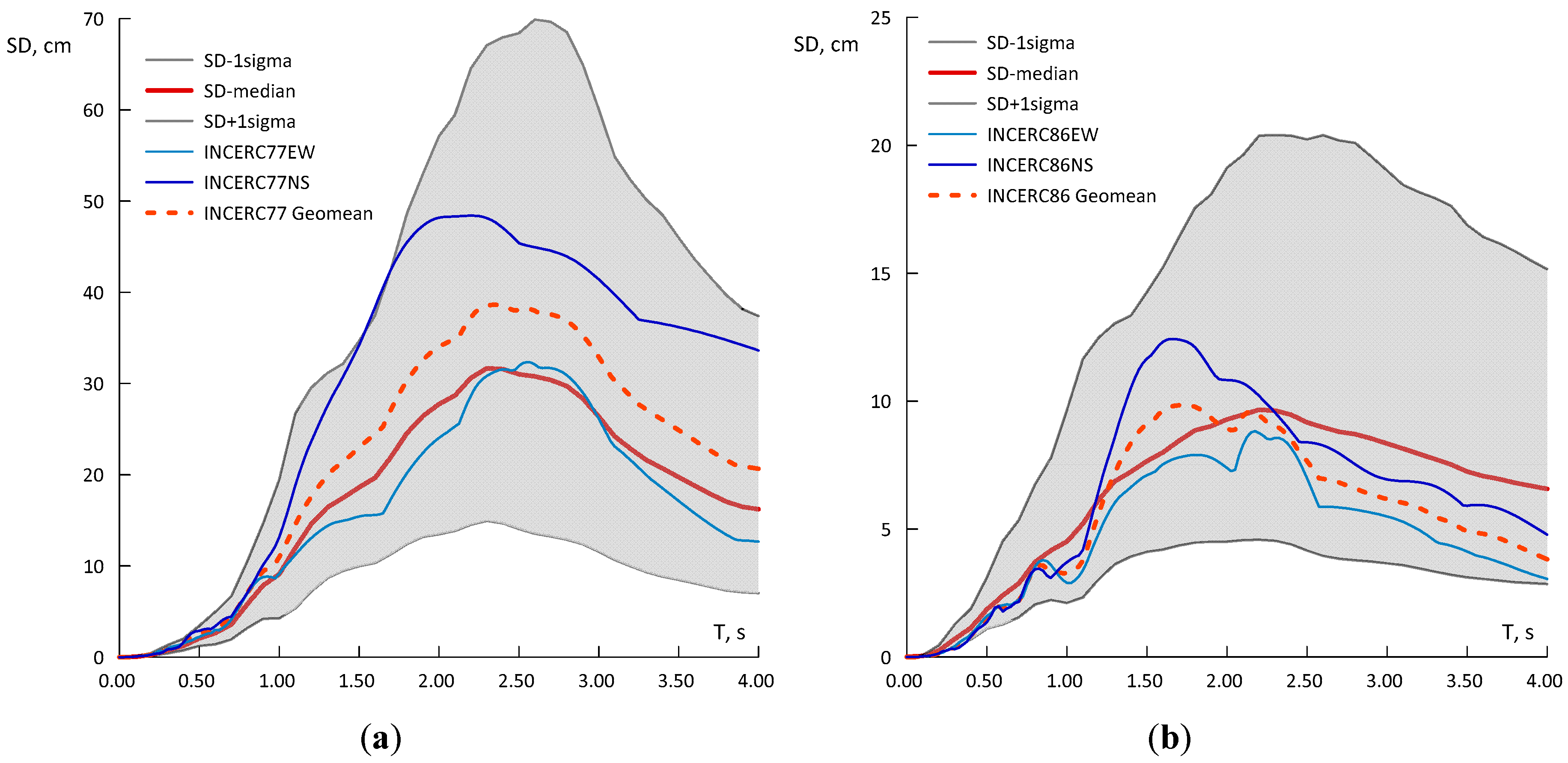
- For prediction of DRS generated by very strong earthquakes, MW ≥ 7.40, the GMPE with the coefficients resulting from the regression of the first set is closer to the observed data for type C soils. The GMPE with quadratic term matches both the spectral shapes and the maximum displacement reasonably well and leads to greater displacement demand than the one shown in Figure 14. A design spectrum should envelope all relevant shapes, considering the appropriate ordinates of the peaks and the variability, through an appropriate number of standard deviations.
3.4. Model Testing
4. Conclusions
Author Contributions
Funding
Acknowledgments
Conflicts of Interest
Appendix A

| T (s) | a | b | c | h | σr2 | σe2 | σ2 | Meannr | Mednr | Stdnr |
|---|---|---|---|---|---|---|---|---|---|---|
| 0.20 | 0.9743 | 0.4724 | 5.39 × 10⁻⁴ | 85.2 | 5.78 × 10⁻² | 1.37 × 10⁻² | 7.15 × 10⁻² | 0.0304 | 0.0943 | 0.9110 |
| 0.40 | 2.3198 | 0.5288 | −2.20 × 10⁻³ | 198.2 | 6.71 × 10⁻² | 6.64 × 10⁻³ | 7.38 × 10⁻² | 0.0414 | 0.0750 | 0.9411 |
| 0.60 | 1.9598 | 0.5393 | −8.33 × 10⁻⁴ | 105.8 | 1.12 × 10⁻¹ | 2.48 × 10⁻³ | 1.14 × 10⁻¹ | 0.0123 | 0.0605 | 0.9680 |
| 0.80 | 1.9577 | 0.5734 | −4.98 × 10⁻⁴ | 102.1 | 1.06 × 10⁻¹ | 1.99 × 10⁻³ | 1.08 × 10⁻¹ | 0.0089 | 0.0544 | 0.9637 |
| 1.00 | 1.8047 | 0.5086 | 5.82 × 10⁻⁴ | 59.6 | 1.04 × 10⁻¹ | 1.13 × 10⁻² | 1.15 × 10⁻¹ | 0.0404 | 0.0896 | 0.9163 |
| 1.50 | 1.9139 | 0.5507 | 3.91 × 10⁻⁴ | 52.8 | 8.72 × 10⁻² | 6.62 × 10⁻³ | 9.38 × 10⁻² | 0.0264 | 0.0738 | 0.9369 |
| 2.00 | 2.0080 | 0.4867 | 3.40 × 10⁻⁴ | 54.8 | 7.55 × 10⁻² | 1.70 × 10⁻² | 9.26 × 10⁻² | 0.0709 | 0.2011 | 0.8895 |
| 2.50 | 2.1979 | 0.3974 | −1.02 × 10⁻⁴ | 64.1 | 6.25 × 10⁻² | 2.33 × 10⁻² | 8.59 × 10⁻² | 0.0994 | 0.1528 | 0.8700 |
| 3.00 | 2.2554 | 0.3990 | −3.15 × 10⁻⁴ | 70.2 | 5.48 × 10⁻² | 2.61 × 10⁻² | 8.10 × 10⁻² | 0.1131 | 0.1188 | 0.8616 |
| 4.00 | 2.4494 | 0.3673 | −6.72 × 10⁻⁴ | 103.0 | 7.30 × 10⁻² | 1.46 × 10⁻² | 8.76 × 10⁻² | 0.0691 | 0.0614 | 0.9025 |
| T (s) | a | b | c | h | σr2 | σe2 | σ2 | Meannr | Mednr | Stdnr |
|---|---|---|---|---|---|---|---|---|---|---|
| 0.20 | 1.0593 | 0.5428 | −3.93 × 10⁻⁴ | 102.9 | 4.08 × 10⁻² | 1.60 × 10⁻² | 5.67 × 10⁻² | 0.0534 | 0.0326 | 0.9321 |
| 0.40 | 1.6011 | 0.7340 | −7.56 × 10⁻⁴ | 112.7 | 4.29 × 10⁻² | 3.19 × 10⁻³ | 4.61 × 10⁻² | 0.0211 | 0.0292 | 0.9278 |
| 0.60 | 2.2368 | 0.8472 | −2.93 × 10⁻³ | 137.3 | 4.15 × 10⁻² | 1.91 × 10⁻² | 6.07 × 10⁻² | 0.0502 | 0.1198 | 0.8650 |
| 0.80 | 2.1411 | 1.0527 | −2.79 × 10⁻³ | 126.3 | 4.20 × 10⁻² | 1.09 × 10⁻² | 5.29 × 10⁻² | 0.0039 | 0.0290 | 0.8338 |
| 1.00 | 1.7332 | 1.1249 | −1.18 × 10⁻³ | 62.5 | 3.42 × 10⁻² | 3.75 × 10⁻² | 7.17 × 10⁻² | 0.0722 | 0.1226 | 0.8098 |
| 1.50 | 2.5936 | 1.1916 | −3.63 × 10⁻³ | 155.6 | 4.96 × 10⁻² | 1.27 × 10⁻² | 6.23 × 10⁻² | 0.0606 | 0.0235 | 0.7777 |
| 2.00 | 2.2520 | 1.2897 | −2.83 × 10⁻³ | 103.4 | 4.90 × 10⁻² | 3.84 × 10⁻² | 8.74 × 10⁻² | 0.1454 | 0.1444 | 0.7392 |
| 2.50 | 2.1502 | 1.2317 | −2.00 × 10⁻³ | 81.7 | 4.52 × 10⁻² | 6.80 × 10⁻² | 1.13 × 10⁻¹ | 0.2015 | 0.1721 | 0.7079 |
| 3.00 | 2.2834 | 1.0479 | −1.70 × 10⁻³ | 88.9 | 5.57 × 10⁻² | 6.86 × 10⁻² | 1.24 × 10⁻¹ | 0.1907 | 0.1798 | 0.7256 |
| 4.00 | 2.3475 | 0.8141 | −1.30 × 10⁻³ | 90.7 | 6.84 × 10⁻² | 4.72 × 10⁻² | 1.16 × 10⁻¹ | 0.1346 | 0.2371 | 0.7931 |
| T (s) | a | b | c | h | σr2 | σe2 | σ2 | Meannr | Mednr | Stdnr |
|---|---|---|---|---|---|---|---|---|---|---|
| 0.20 | 1.0841 | 0.5578 | −2.23 × 10⁻⁴ | 88.3 | 8.15 × 10⁻² | 3.76 × 10⁻² | 1.19 × 10⁻¹ | 0.0336 | 0.0661 | 0.8095 |
| 0.40 | 1.5353 | 0.6640 | −4.13 × 10⁻⁴ | 90.0 | 1.03 × 10⁻¹ | 3.47 × 10⁻² | 1.38 × 10⁻¹ | 0.0484 | 0.0169 | 0.8504 |
| 0.60 | 1.7131 | 0.6964 | −5.89 × 10⁻⁴ | 80.9 | 1.19 × 10⁻¹ | 2.52 × 10⁻² | 1.44 × 10⁻¹ | 0.0323 | 0.0618 | 0.8826 |
| 0.80 | 1.7831 | 0.7259 | −3.70 × 10⁻⁴ | 78.4 | 1.12 × 10⁻¹ | 4.62 × 10⁻² | 1.58 × 10⁻¹ | 0.0221 | 0.0008 | 0.8135 |
| 1.00 | 1.6559 | 0.7388 | 3.97 × 10⁻⁴ | 49.1 | 1.08 × 10⁻¹ | 4.19 × 10⁻² | 1.50 × 10⁻¹ | 0.0205 | 0.0369 | 0.8197 |
| 1.50 | 1.7453 | 0.8348 | −5.91 × 10⁻⁶ | 51.2 | 8.64 × 10⁻² | 3.68 × 10⁻³ | 9.00 × 10⁻² | 0.0107 | 0.1041 | 0.9654 |
| 2.00 | 1.7491 | 0.8445 | −5.95 × 10⁻⁵ | 52.0 | 8.04 × 10⁻² | 3.63 × 10⁻² | 1.17 × 10⁻¹ | 0.0733 | 0.2136 | 0.8254 |
| 2.50 | 1.8158 | 0.8383 | −3.87 × 10⁻⁴ | 62.6 | 6.95 × 10⁻² | 5.32 × 10⁻² | 1.23 × 10⁻¹ | 0.1175 | 0.1905 | 0.7903 |
| 3.00 | 1.8308 | 0.8688 | −5.16 × 10⁻⁴ | 68.4 | 6.50 × 10⁻² | 5.79 × 10⁻² | 1.23 × 10⁻¹ | 0.1359 | 0.2026 | 0.7784 |
| 4.00 | 1.8552 | 0.8807 | −5.74 × 10⁻⁴ | 80.9 | 7.61 × 10⁻² | 6.92 × 10⁻² | 1.45 × 10⁻¹ | 0.1532 | 0.2343 | 0.7880 |
| T (s) | a | b | c | h | σr2 | σe2 | σ2 | Meannr | Mednr | Stdnr |
|---|---|---|---|---|---|---|---|---|---|---|
| 0.20 | 3.0994 | 0.6661 | −5.70 × 10⁻³ | 278.0 | 4.47 × 10⁻² | 3.08 × 10⁻² | 7.55 × 10⁻² | 0.0610 | 0.2030 | 0.9760 |
| 0.40 | 6.9703 | 0.8816 | −1.00 × 10⁻² | 483.3 | 4.16 × 10⁻² | 5.17 × 10⁻² | 9.34 × 10⁻² | 0.1374 | 0.3661 | 0.9482 |
| 0.60 | 9.1643 | 0.9443 | −1.26 × 10⁻² | 534.6 | 3.82 × 10⁻² | 7.56 × 10⁻² | 1.14 × 10⁻¹ | 0.0743 | 0.1374 | 0.8699 |
| 0.80 | 3.5193 | 1.0032 | −5.55 × 10⁻³ | 239.0 | 4.33 × 10⁻² | 8.46 × 10⁻² | 1.28 × 10⁻¹ | 0.0086 | 0.0062 | 0.8242 |
| 1.00 | 2.8424 | 1.0528 | −4.04 × 10⁻³ | 169.3 | 3.99 × 10⁻² | 9.75 × 10⁻² | 1.37 × 10⁻¹ | 0.0835 | 0.0959 | 0.8115 |
| 1.50 | 3.3158 | 1.1715 | −5.05 × 10⁻³ | 205.3 | 4.37 × 10⁻² | 7.10 × 10⁻² | 1.15 × 10⁻¹ | 0.0748 | 0.1774 | 0.8594 |
| 2.00 | 3.0047 | 1.2101 | −4.54 × 10⁻³ | 177.3 | 4.15 × 10⁻² | 5.09 × 10⁻² | 9.24 × 10⁻² | 0.0080 | 0.1074 | 0.9204 |
| 2.50 | 2.8699 | 1.2264 | −4.20 × 10⁻³ | 167.4 | 4.10 × 10⁻² | 5.52 × 10⁻² | 9.63 × 10⁻² | 0.0166 | 0.1358 | 0.9195 |
| 3.00 | 2.7517 | 1.2277 | −3.79 × 10⁻³ | 165.2 | 4.73 × 10⁻² | 5.38 × 10⁻² | 1.01 × 10⁻¹ | 0.0133 | 0.0967 | 0.9319 |
| 4.00 | 2.9025 | 1.2132 | −4.11 × 10⁻³ | 187.1 | 5.49 × 10⁻² | 5.50 × 10⁻² | 1.10 × 10⁻¹ | 0.0208 | 0.0342 | 0.9336 |
References
- Frohlich, C. Deep Earthquakes; Cambridge University Press: Cambridge, UK, 2006; pp. 535–541. [Google Scholar]
- Ismail-Zadeh, A.; Mueller, B.; Schubert, G. Three-dimensional numerical modeling of contemporary mantle flow and tectonic stress beneath the earthquake-prone southeastern Carpathians based on integrated analysis of seismic, heat flow, and gravity data. Phys. Earth Planet. Inter. 2005, 149, 81–98. [Google Scholar] [CrossRef]
- Radulian, M.; Mândrescu, N.; Panza, G.F.; Popescu, E.; Utale, A. Characterization of Seismogenic Zones of Romania. Pure Appl. Geophys. 2000, 157, 57–77. [Google Scholar] [CrossRef]
- Lungu, D.; Aldea, A.; Arion, C.; Văcăreanu, R. Hazard, Vulnerabilitate și Risc Seismic. In Construcții Amplasate în Zone cu Mișcări Seismice Puternice; Dubină, D., Lungu, D., Eds.; Editura Orizonturi Universitare: Timișoara, Romania, 2003; pp. 21–157. [Google Scholar]
- Wells, D.L.; Coppersmith, K.J. New Empirical Relationships among Magnitude, Rupture Length, Rupture Width, Rupture Area, and Surface Displacement. Bull. Seismol. Soc. Am. 1994, 84, 974–1002. [Google Scholar]
- Orphal, D.L.; Lahoud, J.A. Prediction of peak ground motion from earthquakes. Bull. Seismol. Soc. Am. 1974, 64, 1563–1574. [Google Scholar]
- Douglas, J. Ground Motion Prediction Equations 1964–2019. Available online: http://www.gmpe.org.uk (accessed on 3 February 2020).
- Bommer, J.J.; Elnashai, A.S.; Chlimintzas, G.O.; Lee, D. Review and Development of Response Spectra for Displacement-Based Seismic Design; ESEE Report 98-3; Department of Civil Engineering, Imperial College: London, UK, 1998. [Google Scholar]
- Faccioli, E.; Paolucci, R.; Rey, J. Displacement Spectra for Long Periods. Earthq. Spectra 2004, 20, 347–376. [Google Scholar] [CrossRef]
- Akkar, S.; Bommer, J.J. Prediction of elastic displacement response spectra in Europe and the Middle East. Earthq. Eng. Struct. Dyn. 2007, 36, 1275–1301. [Google Scholar] [CrossRef]
- Cauzzi, C.; Faccioli, E. Broadband (0.05 to 20 s) prediction of displacement response spectra based on worldwide digital records. J. Seismol. 2008, 12, 453–475. [Google Scholar] [CrossRef]
- Faccioli, E.; Cauzzi, C.; Paolucci, R.; Vanini, M.; Villani, M.; Finazzi, D. Long Period Strong Ground Motion and its Use as Input to Displacement Based Design. In Earthquake Geotechnical Engineering; Pitilakis, K.D., Ed.; Springer: Dordrecht, The Netherlands, 2007; pp. 23–51. [Google Scholar]
- Faccioli, E.; Villani, M. Seismic Hazard Mapping for Italy in Terms of Broadband Displacement Spectra. Earthq. Spectra 2009, 25, 515–539. [Google Scholar] [CrossRef]
- Hassani, N.; Amiri, G.; Bararnia, M.; Sinaeian, F. Ground motion prediction equation for inelastic spectral displacement in Iran. Sci. Iran. B 2017, 24, 164–182. [Google Scholar] [CrossRef] [Green Version]
- Bindi, D.; Kotha, S.R.; Weatherill, G.; Lanzano, G.; Luzi, L.; Cotton, F. The pan-European engineering strong motion (ESM) flatfile: Consistency check via residual analysis. Bull. Earthq. Eng. 2019, 17, 583–602. [Google Scholar] [CrossRef]
- Lungu, D.; Demetriu, S.; Radu, C.; Coman, O. Uniform hazard response spectra for Vrancea earthquakes in Romania. In Proceedings of the 10th European Conference on Earthquake Engineering, Balkema, Rotterdam, 28 August–2 September 1994; pp. 365–370. [Google Scholar]
- Radu, C.; Lungu, D.; Demetriu, S.; Coman, O. Recurrence, attenuation and dynamic amplification for intermediate depth Vrancea earthquakes. In Proceedings of the XXIV General Assembly of the ESC, Athens, Greece, 19–24 September 1994; Volume 3, pp. 1736–1745. [Google Scholar]
- Stamatovska, S.; Petrovski, D. Empirical attenuation acceleration laws for Vrancea intermediate earthquakes. In Proceedings of the 11th World Conference on Earthquake Engineering, Acapulco, Mexico, 23–28 June 1996. [Google Scholar]
- Sokolov, V.; Bonjer, K.P.; Wenzel, F.; Grecu, B.; Radulian, M. Ground-motion prediction equations for the intermediate depth Vrancea (Romania) earthquakes. Bull. Earthq. Eng. 2008, 6, 367–388. [Google Scholar] [CrossRef]
- Lungu, D.; Aldea, A.; Arion, C.; Demetriu, S.; Cornea, T. Microzonage Sismique de la ville de Bucarest-Roumanie. Cah. Tech. L’Assoc. Fr. Genie Parasismique 2000, 20, 31–63. [Google Scholar]
- MDRAP. P100-1/2013—Romanian Seismic Code; Ministerul Dezvoltării Regionale și a Administrației Publice: București, România, 2013. (In Romanian)
- Vacareanu, R.; Demetriu, S.; Lungu, D.; Pavel, F.; Arion, C.; Iancovici, M.; Aldea, A.; Neagu, C. Empirical ground motion model for Vrancea intermediate-depth seismic source. Earthq. Struct. 2014, 6, 141–161. [Google Scholar] [CrossRef]
- Vacareanu, R.; Radulian, M.; Iancovici, M.; Pavel, F.; Neagu, C. Fore-Arc and Back-Arc Ground Motion Prediction Model for Vrancea Intermediate Depth Seismic Source. J. Earthq. Eng. 2015, 19, 535–562. [Google Scholar] [CrossRef]
- Strong Motion Seismograph Networks—K-NET, KiK-Net—National Research Institute for Earth Science and Disaster Resilience. Available online: http://www.kyoshin.bosai.go.jp/ (accessed on 30 January 2017).
- Borcia, I.S. Procesarea Înregistrărilor Mișcărilor Seismice Vrâncene Puternice; Editura Societății Academice Matei-Teiu Botez: Iași, Romania, 2008. (In Romanian) [Google Scholar]
- Lungu, D.; Văcăreanu, R.; Aldea, A.; Arion, C. Advanced Structural Analysis; Conspress: Bucharest, Romania, 2000. [Google Scholar]
- CEN. European Standard EN 1998-1:2004 Eurocode 8: Design of Structures for Earthquake Resistance, Part 1: General Rules, Seismic Actions and Rules for Buildings; Comite Europeen de Normalisation: Brussels, Belgium, 2004. [Google Scholar]
- Neagu, C.; Arion, C.; Aldea, A.; Văcăreanu, R.; Pavel, F. Ground Types for Seismic Design in Romania. In Proceedings of the 6th National Conference on Earthquake Engineering & 2nd National Conference on Earthquake Engineering and Seismology, București, Romania, 14–17 June 2017; Conspress: București, Romania, 2017. [Google Scholar]
- Allen, T.; Wald, D. Topographic Slope as a Proxy for Seismic Site-Conditions (Vs30) and Amplification around the Globe; U.S. Geological Survey Open-File Report 2007-1357; Geological Survey (U.S.): Reston, VA, USA, 2007; 69p.
- United States Geological Survey, Vs30 Data. Available online: https://earthquake.usgs.gov/data/vs30/ (accessed on 13 July 2017).
- Boore, D. Estimating Vs30 (or NEHRP classes) from shallow Velocity Models (Depths < 30 m). Bull. Seismol. Soc. Am. 2004, 94, 591–597. [Google Scholar]
- Boore, D. Available online: http://www.daveboore.com/data_online.html (accessed on 13 July 2017).
- Joyner, W.; Boore, D. Methods for Regression Analysis of Strong-Motion Data. Bull. Seismol. Soc. Am. 1993, 83, 469–487. [Google Scholar]
- Joyner, W.; Boore, D. Errata—Methods for Regression Analysis of Strong-Motion Data. Bull. Seismol. Soc. Am. 1994, 84, 955–956. [Google Scholar]
- Brillinger, D.; Preisler, H. An exploratory analysis of the Joyner-Boore attenuation data. Bull. Seismol. Soc. Am. 1984, 74, 1441–1450. [Google Scholar]
- Boore, D.; Joyner, W.; Fumal, T. Equations for Estimating Horizontal Response Spectra and Peak Acceleration from Western North American Earthquakes: A Summary of Recent Work. Seismol. Res. Lett. 1997, 68, 128–153. [Google Scholar] [CrossRef]
- Boore, D.M. Equations for Estimating Horizontal Response Spectra and Peak Acceleration from Western North American Earthquakes: A Summary of Recent Work. Erratum. Seismol. Res. Lett. 2005, 76, 368–369. [Google Scholar] [CrossRef]
- Seismosignal Software. Available online: https://seismosoft.com/product/seismosignal/ (accessed on 20 December 2017).
- Pavel, F.; Vacareanu, R.; Calotescu, I.; Coliba, V. Design Displacement Response for Southern and Eastern Romania. In Proceedings of the 16th World Conference on Earthquake, 16WCEE 2017, Santiago, Chile, 9–13 January 2017. [Google Scholar]
- ViewWave Software. Available online: https://smo.kenken.go.jp/~kashima/viewwave (accessed on 27 November 2016).
- Văcăreanu, R.; Pavel, F.; Aldea, A.; Arion, C.; Neagu, C. Elemente de Analiză a Hazardului Seismic; Conspress: București, Romania, 2015. [Google Scholar]
- Scherbaum, F.; Delavaud, E.; Riggelsen, C. Model Selection in Seismic Hazard Analysis: An Information-Theoretic Perspective. Bull. Seismol. Soc. Am. 2009, 99, 3234–3247. [Google Scholar] [CrossRef]


| Date (year/month/day) | Local Time | Latitude (°N) | Longitude (°E) | Focal Depth (km) | Mw | Number of Horizontal Components | Country of Origin |
|---|---|---|---|---|---|---|---|
| 1977/03/04 | 19:21:54 | 45.77 | 26.76 | 94 | 7.4 | 4 | RO |
| 1986/08/30 | 21:28:37 | 45.52 | 26.49 | 131 | 7.1 | 70 | RO |
| 1990/05/30 | 10:40:06 | 45.83 | 26.89 | 91 | 6.9 | 92 | RO |
| 1990/05/31 | 00:17:48 | 45.85 | 26.91 | 87 | 6.4 | 66 | RO |
| 2004/10/27 | 20:34:36 | 45.84 | 26.63 | 105 | 6.0 | 92 | RO |
| 2005/05/14 | 01:53:21 | 45.64 | 26.53 | 149 | 5.5 | 14 | RO |
| 2005/06/18 | 15:16:42 | 45.72 | 26.66 | 154 | 5.2 | 14 | RO |
| 2009/04/25 | 17:18:48 | 45.68 | 26.62 | 110 | 5.4 | 10 | RO |
| 2013/10/06 | 01:37:21 | 45.67 | 26.58 | 135 | 5.2 | 108 | RO |
| 2001/12/02 | 22:02:00 | 39.40 | 141.26 | 122 | 6.4 | 6 | JAP |
| 2003/05/26 | 18:24:00 | 38.81 | 141.68 | 71 | 7.0 | 24 | JAP |
| 2005/07/23 | 16:35:00 | 36.58 | 140.14 | 73 | 6.0 | 6 | JAP |
| 2008/07/24 | 00:26:00 | 39.73 | 141.63 | 108 | 6.8 | 16 | JAP |
| 2011/04/07 | 23:32:00 | 38.20 | 141.92 | 66 | 7.1 | 18 | JAP |
| 2013/02/02 | 23:17:00 | 42.70 | 142.23 | 102 | 6.5 | 4 | JAP |
| Event (year/month/day) | MW | PGA, cm/s2 | SDmax, cm | ||
|---|---|---|---|---|---|
| EW | NS | EW | NS | ||
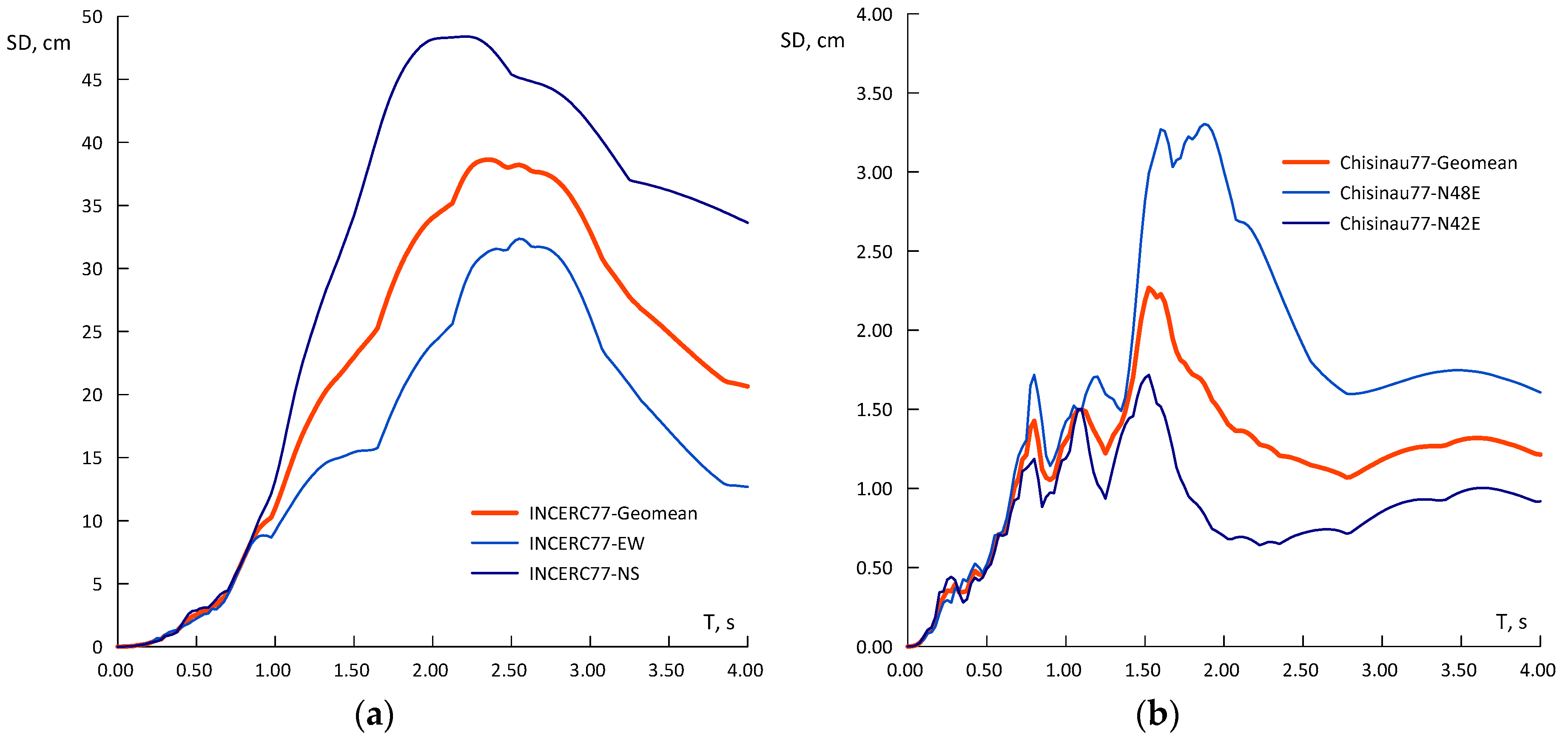
| 1977.03.04 | 7.4 | 188 | 207 | 32.4 | 48.4 |
| 1986.08.31 | 7.1 | 109 | 96 | 8.8 | 12.4 |
| 1990.05.30 | 6.9 | 99 | 66 | 9.3 | 3.4 |
© 2020 by the authors. Licensee MDPI, Basel, Switzerland. This article is an open access article distributed under the terms and conditions of the Creative Commons Attribution (CC BY) license (http://creativecommons.org/licenses/by/4.0/).
Share and Cite
Olteanu, P.; Vacareanu, R. Ground Motion Model for Spectral Displacement of Intermediate-Depth Earthquakes Generated by Vrancea Seismic Source. Geosciences 2020, 10, 282. https://doi.org/10.3390/geosciences10080282
Olteanu P, Vacareanu R. Ground Motion Model for Spectral Displacement of Intermediate-Depth Earthquakes Generated by Vrancea Seismic Source. Geosciences. 2020; 10(8):282. https://doi.org/10.3390/geosciences10080282
Chicago/Turabian StyleOlteanu, Paul, and Radu Vacareanu. 2020. "Ground Motion Model for Spectral Displacement of Intermediate-Depth Earthquakes Generated by Vrancea Seismic Source" Geosciences 10, no. 8: 282. https://doi.org/10.3390/geosciences10080282