Article

Mapping Landslide Prediction through a GIS-Based Model: A Case Study in a Catchment in Southern Italy

by
Federico Valerio Moresi
1,
Mauro Maesano
1,2,
Alessio Collalti
1,2,
Roy C. Sidle
3,4,5,
Giorgio Matteucci
6 and
Giuseppe Scarascia Mugnozza
1,*
1
Department of Innovation in Biological, Agro-Food and Forest Systems, University of Tuscia, 01100 Viterbo, Italy
2
Institute for Agricultural and Forest Systems in the Mediterranean, National Research Council of Italy, 00100 Rome, Italy
3
Mountain Societies Research Institute, University of Central Asia, Khorog 736000, Tajikistan
4
Institute of Global Innovation Research, Tokyo University of Agriculture and Technology, Tokyo 183-8538, Japan
5
Sustainability Research Centre, University of the Sunshine Coast, Sippy Downs, QLD 4556, Australia
6
Institute of BioEconomy (IBE), 50019 Sesto Fiorentino (FI), Italy
*
Author to whom correspondence should be addressed.
Geosciences 2020, 10(8), 309; https://doi.org/10.3390/geosciences10080309
Submission received: 30 June 2020 / Revised: 7 August 2020 / Accepted: 10 August 2020 / Published: 12 August 2020
(This article belongs to the Special Issue Innovative Strategies for Sustainable Mitigation of Landslide Risk)

Abstract

:
Shallow landslides are an increasing concern in Italy and worldwide because of the frequent association with vegetation management. As vegetation cover plays a fundamental role in slope stability, we developed a GIS-based model to evaluate the influence of plant roots on slope safety, and also included a landslide susceptibility map. The GIS-based model, 4SLIDE, is a physically based predictor for shallow landslides that combines geological, topographical, and hydrogeological data. The 4SLIDE combines the infinite slope model, TOPMODEL (for the estimation of the saturated water level), and a vegetation root strength model, which facilitates prediction of locations that are more susceptible for shallow landslides as a function of forest cover. The aim is to define the spatial distribution of Factor of Safety (FS) in steep-forested areas. The GIS-based model 4SLIDE was tested in a forest mountain watershed located in the Sila Greca (Cosenza, Calabria, South Italy) where almost 93% of the area is covered by forest. The sensitive ROC analysis (Receiver Operating Characteristic) indicates that the model has good predictive capability in identifying the areas sensitive to shallow landslides. The localization of areas at risk of landslides plays an important role in land management activities because landslides are among the most costly and dangerous hazards.

Graphical Abstract

1. Introduction

Landslides are defined as mass movements of soil and rocks along a slope. Landslides occur when slopes undergo a decrease in the shear strength of the hillside material due to an increase in the shear stress, or due to a combination of natural ecosystem processes and anthropogenic activities [1,2]. In some cases, human activities can trigger or, more often, they can accelerate the dynamics of natural processes by modifying the threshold of occurrence of landslides, thus potentially increasing risks for people. A frequent determinant of these processes consists of extreme weather events in geomorphologically unstable areas. Furthermore, land use changes and different land management practices can interact with those factors due to their influence on soil hydrological response, thus increasing hazard risk [3,4,5,6]. In 2016, worldwide, natural disasters caused 8733 deaths, affected 569.4 million people, and caused US$ 154 billion in damages. Particularly, hydrological disasters include the largest share of accidents caused by natural events (51.7%), while the geophysical disasters represent a smaller fraction, by 9.1% [7]. According to the Italian inventory of floods and landslides (IFFI—Inventario dei Fenomeni Franosi in Italia), more than 50,593 people died in 2580 floods and landslides between 1979 and 2002 (floods casualties have totaled 38,242 while those caused by landslides were 12,351) [8]. The IFFI inventory includes about 500,000 landslides affecting an area of about 21,000 km2, corresponding to 6.9% of the national territory [9]. In Italy, landslide risk reflects the geomorphology of the country; in fact, about 75% of the Italian territory is comprised of mountainous and hilly terrain [10]. In these areas, forests play a fundamental role in preventing natural hazards and their management is important at different spatial scales [11,12,13]. In past centuries, forests have protected people from many natural hazards [1,14,15]. Slopes benefit from forest cover in different ways: through mechanical reinforcement of soil by roots, improvement of soil structure, and soil water removal by evapotranspiration. The reinforcement level depends on terrain characteristics, rocky substrate, and vegetation type. Such a mitigating role can be estimated through models that evaluate the effect of mechanical reinforcement of roots in the soil [16,17] in addition to being able to generate probability maps of landslide occurrence under different scenarios of forest management. In the past, several methodologies to generate landslide susceptibility maps have been outlined [1,18,19,20,21,22] and several models have been developed. The numerical and deterministic models are generally used for evaluating the landslide susceptibility and to forecast their evolution based on remote sensing data within a Geographical Information System (GIS) [18,19]. At the same time, GIS-based analyses have been employed to develop landslide susceptibility maps. These GIS analyses are also useful for generating landslide inventory maps and for monitoring landslide deformation [23]. Many of these models are difficult to access, while others are open source; however, most are not user-friendly for non-specialists because they are scripting-oriented and rather complex to apply [18]. In addition, many of these models are not freely available.
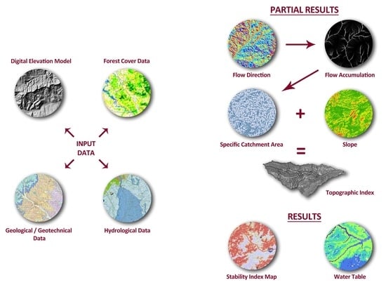
In response to these issues, in this study, a new tool in a GIS environment called “4SLIDE” has been developed to identify potentially hazardous areas of landslide occurrence. The tool uses not only numerical values for input data but also raster maps. Indeed, if the user has spatially distributed geotechnical data, maps can be created where each cell corresponds to site-specific data—e.g., soil cohesion, root cohesion, internal angle of friction. Specifically, the tool combines different models for analyzing geological, topographical, and hydrological data for calculating the Factor of Safety Index (FS) index. In this context, 4SLIDE is a GIS-based model that uses a combination of LiDAR and field-survey data to compute FS to locate hazard areas and to create a map of stability index aimed at identifying areas susceptible to landslides as a useful tool for land governance and strategic planning [24]. 4SLIDE was tested and validated in an experimental forested catchment “Bonis”, located in the mountain area of Sila Greca, Calabria, South Italy.

2. Materials and Methods

2.1. The 4SLIDE

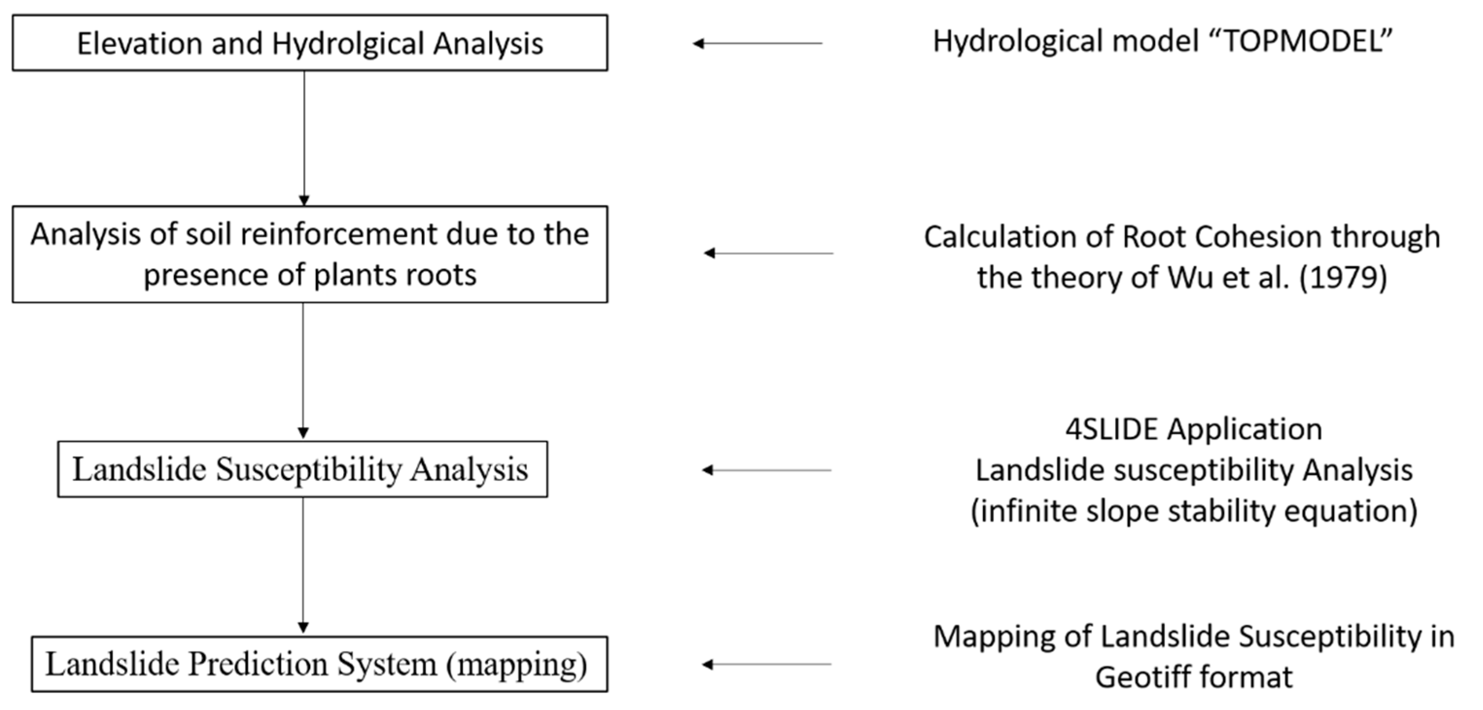
The 4SLIDE GIS-based model was set up as an add-on toolbox component to ESRI’s ArcGIS© 10.3 for Desktop for creating a toolbox. The 4SLIDE tool uses the infinite slope stability equation [25] for calculating the Factor of Safety Index and it applies the hydrological model “TOPMODEL” (a TOPography based hydrological MODEL) [26] for evaluating the landslide risk at the catchment scale. In addition, this model considers soil reinforcement due to the presence of plants roots through a vegetation root strength model according to the theory presented in Wu et al. [27]. The main output of the tool is the Factor of Safety (FS) raster map called a “soil stability map”. An overview of the workflow methodology of 4SLIDE in ArcGIS environment for landslide hazard prediction is shown in Figure 1.
The soil stability map provides, for each pixel, a value used to classify the terrain in risk classes subdivided in terms of the Factor of Safety Index (Table 1). In Figure A1, the GIS-based model development procedure was described.

2.2. Factor of Safety Index

The FS index is defined as the ratio of stresses resisting failure (Sr) to the stress required to bring the slope into a state of limit equilibrium (SL) along a failure surface according to the infinite slope stability equation (ISSE). This limit equilibrium analysis can be applied for all types of failure slip surfaces. The most useful analytical method for forested slopes is the planar infinite slope analysis [28]. This analysis assumes that the thickness of the soil mantle is small compared to the slope length and the failure plane is parallel to the slope [27,29,30]. For forested slopes with water tables less than or equal to soil depth (in meters), the FS index is [3]:
F S = C + c R + { [ ( Z h ) γ m + h γ s a t ] Z cos 2 β u + W cos 2 β } tan Φ [ ( Z h ) γ m + h γ s a t ] sin β cos β + W sin β
where cR is the cohesion attributed to root systems (kPa), γm is the unit weight of soil at field moisture content (kN m−3), γsat is the unit weight of saturated soil (kN m−3), Z the vertical soil thickness (m), h is the vertical height of the water table (m), β is the slope angle (in radians), and W the vegetation surcharge (kPa). In areas with FS < 1.3, there is a probability of failure.

2.3. Hydrological Model

The TOPMODEL approach has become widely used for hydrological catchment modeling [26,31,32]. Different than other models, TOPMODEL does not divide the catchment into homogeneous units, but rather employs distribution functions to represent the catchment’s natural heterogeneity and its effects on hydrological processes. Therefore, the distribution of wetness throughout a catchment can be simulated easily and with low computational demand. These developments follow field observations that show that higher soil moisture or areas of surface saturation tend to occur in convergent hollows. It has also been reported that landslides most commonly originate in areas of topographic convergence [17,26]. As per Beven and Kirkby [32], the index of hydrological similarity (I) is based on the topographic index of Kirkby and Statham [33] and defined as:
I = ln ( a tan β )
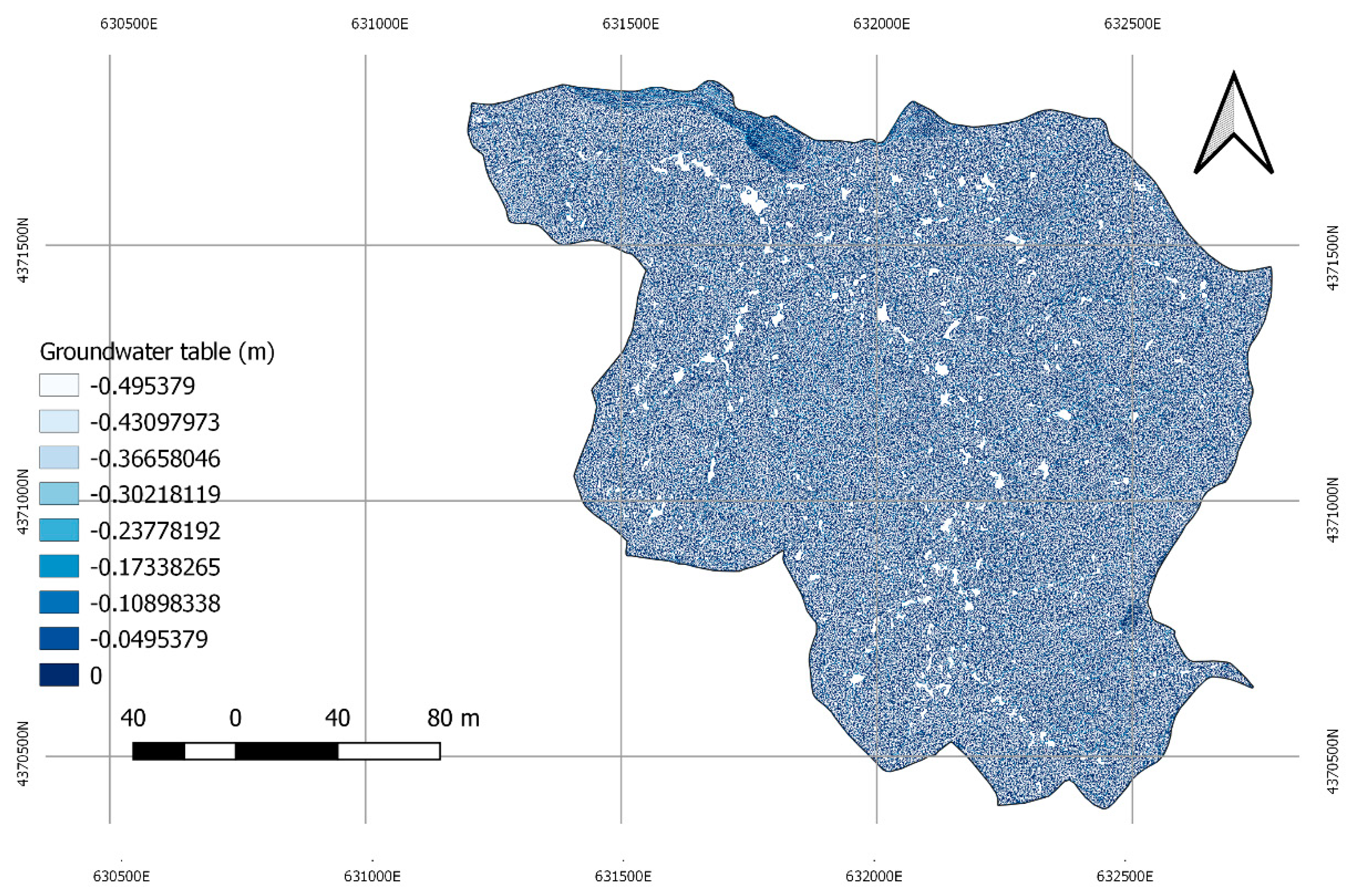
where, a is the specific catchment area, defined as upslope area per unit contour length (m), and β is the slope angle of the ground surface (Figure A6). This index describes the tendency of water to accumulate (a) and to be moved downslope by gravitational forces (β). TOPMODEL can be used for determination of the groundwater levels (z) (Figure A7).; this theory assumes that transmissivity decreases exponentially with increasing depth to the groundwater table z (meter below surface), the hydraulic gradient is equal to the surface gradient (β), and lateral flow in the unsaturated zone can be neglected. A mean depth to the water table, z ¯ at each location i, is given by the equation:
z ¯ = 1 A   z i d A = 1 f A I i ln R   d A =     1 f ( I ¯ ln T ¯ + ln R )
where, Ti (m2 t−1) is the transmissivity if the groundwater level is at the ground surface, f (m−1) is a shape factor describing the exponential decrease of conductivity with soil depth, R is recharge, and A is the catchment area.

2.4. The Vegetation Root Strength Model

Plants represent an effective means of defense against surface erosion. The increase in soil shear strength due to the presence of roots was assessed according to the model presented by Wu et al. [27]. This model allows for simple and quick calculation of soil reinforcement by roots using tensile strength and root distribution information, resulting in additional cohesion [34]. If the soil is rooted, the increased soil resistance to slides can be expressed as an additional cohesion cR (kPa) [35,36] that increases shear strength due to the presence of roots:
c R = k k i = 1 N ( T R a r ) i
where, TR is the tensile strength and ar is the Root Area Ratio (RAR), both specified per tree diameter class i, N is the number of classes considered, k′ is the factor accounting for decomposition of root tensile strength according to the bending angle of roots with respect to the shear plane, and k″ is a reduction factor accounting for the non-simultaneous breaking of roots [20].

2.5. 4SLIDE Tool Implementation

4SLIDE GIS-based model was implemented in ModelBuilder application. This is an easy-to-use application for creating, editing, and managing models in ArcGIS Desktop 10© (Esri). The data processing workflow for defining the FS index map is shown in Figure 1. In the first phase, the fundamental data are collected and inserted within the Model Builder. Subsequently, the internal tools of ArcGIS are used to determine the morphological and hydrological parameters needed to run the TOPMODEL equations. Lastly, the root cohesion parameters are inserted into Model Builder and, through the Raster Calculator tool (ArcGIS tool), the infinite slope stability equation is employed (Figure A1). At this stage, the model computes the Factor of Safety index and a map is created.

Input and Output Tool Data

The 4SLIDE tool requires a digital terrain model (DTM) for calculating the topographic factors like slope angle in radians (rad) and the drainage network. The hydrological data required by the model are: (i) transmissivity (m2 hr−1) (the rate at which groundwater flows horizontally through an aquifer or soil), (ii) the effective drainable porosity (the fraction of voids per unit volume), (iii) the discharge of watershed outlet (m3 s−1) (the amount of fluid that crosses a section of the area A in the time unit), and (iv) basin area (m2). Moreover, the model requires the following soil data: (a) soil cohesion (in kPa), (b) internal angle of friction (radians), (c) dry unit soil weight (kN m−3), (d) wet unit soil weight (kN m−3), and (e) vertical soil depth (m). The last input parameter is root cohesion (kPa) for plants. Here, a homogeneous value for the entire study area or a raster map with different values can be used (Figure A2). The model uses either numerical values (N.V.) (across all cells) or a raster map (a value that varies across different cells) for each parameter. The values that can be changed by the user to generate different simulations in the dialog box are reported in Table 2.
The output of 4SLIDE tool is a FS index map in the form of a raster file. FS values < 1 indicate slope failure (i.e., a cell where a landslide is highly likely), while values < 1.3 indicate unstable conditions. For display purposes, in this study, the FS index was grouped into five classes according to Pack et al. [37] (Table 1).

2.6. Case Study

Landslides are very diffused in large areas of the Italian territory [38], in particular, in the Calabria region (Southern Italy). In fact, in this territory, a great number of sites are quite prone to landsliding, due to the combination of their geological, morphological, climatic, and land management features [39,40]. This region is also characterized by a complex orography and generally small river basins that respond rapidly to rainfall. Intense meteorological events combined with these attributes of the territory give rise to violent shallow landslide phenomena characterized by rapid dynamics. About 70% of the rainfall occurs from October to March, with average annual precipitation ranging from 1000 to 2000 mm y−1 [41]. The study area is a forest catchment (coordinate of the center of the catchment: WGS 84/UTM zone 33N—EPSG: 32633) called “Bacino del Bonis”, located in the border area between the municipalities of Acri and Longobucco (Figure 2) [42].
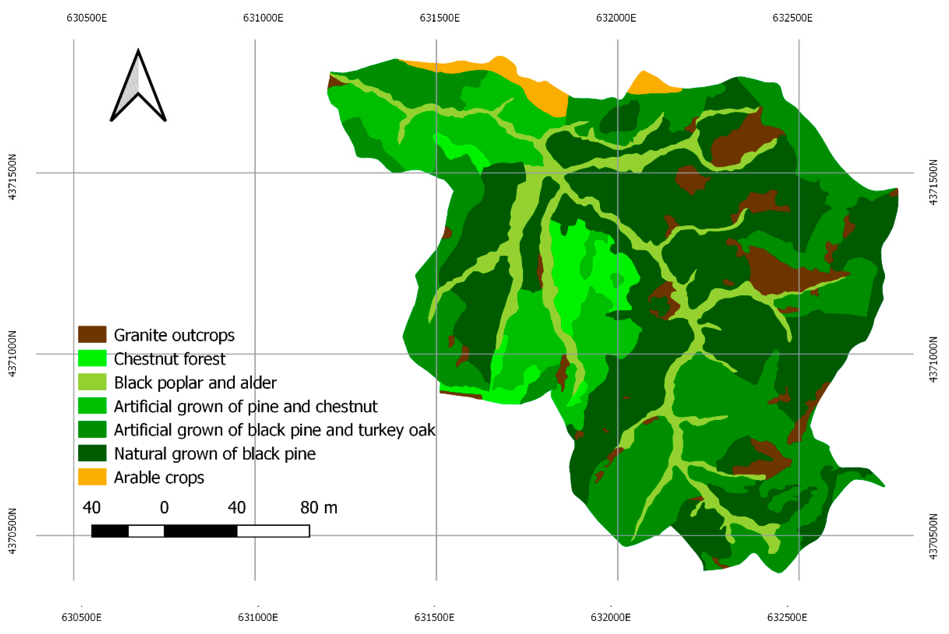
The basin was instrumented in 1986 with three mechanical rain gauges (with tipping buckets, data compiled in 20-min intervals) located at the basin outlet (975 m a.s.l.) and at representative sites within the north-eastern (Petrarella: 1258 m a.s.l.) and southwestern (Don Bruno: 1175 m a.s.l.) parts of the catchment. Runoff was measured at the catchment outlet using a Thomson weir (capable of measuring discharges up to 17 m3 s−1) equipped with a mechanical stage recorder. The basin area is 1385 km2, most of which is forested with an incised stream network. The area is covered by Calabrian pine (Pinus laricio Poiret) with small areas of mixed stands of chestnut (Castanea sativa Mill.) and alder riparian forest (Alnus glutinosa (L.) Gaertn) (Figure 3).
The main stream has long steep slopes varying from 35 to 40% with the presence of several waterfalls and some isolated pools. The geology throughout the territory consists of four major complexes of different ages. The oldest complex is comprised of an acid igneous and metamorphic unit (Sila unit) of Paleozoic age and calcareous unit of Mesozoic age [43]. These rocks are covered by a Paludi formation of lower Miocene age [44], followed by a sedimentary succession of mio-pliocene [45] and; Quaternary sediments [46,47]. A complex of acidic intrusive plutonic rocks mainly characterizes the study basin. Soils are predominantly coarse-textured colluvium derived from volcanic rocks and classified as ultic haploxeralfs according to soil taxonomy [47]. Soil depth is shallow, with an average depth of about 1 m, and highly permeable to water. The water table rapidly responds during rainfall, rising and falling in response to rain intensity. The average annual precipitation is 1250 mm year−1 and average air temperature is 8.8 °C [47], with a typical mountain-Mediterranean climate regime, characterized by cool and wet winters and warm and dry summers. For this study, the soil properties considered are: soil cohesion, internal friction angle, unconfined compressive strength, unit weight, and saturated hydraulic conductivity (Table 3).
These soil data were determinate by 135 soil samples taken within the study area [48] (Figure A3).

2.7. Calibration and Sensitivity Analysis

The 4SLIDE tool was applied in the study area and several input data for generating the FS index map were used. Firstly, high-resolution Digital Terrein Model (DTM) (Figure A5) derived from a LiDAR survey (Figure A4) conducted in the ALForLab project (www.alforlab.eu) were used. For vegetation, root cohesion data is described in Moresi et al. [36], while the geotechnical parameters were derived from Belloti & Selleri [49] (Table 3). The soil map was made after a detailed geological survey inside Bonis basin (Figure 4). This map is a product of the ALFORLAB project created by a kriging geostatistics algorithm in QGIS software.
Rainfall data were collected from the Cecita (CS) weather station, the nearest station to the study area (~10 km). A sensitivity analysis of the 4SLIDE parameters was also conducted. The 4SLIDE sensitivity was assessed by analyzing the changes with respect to a standard value resulting from the variation of the generic i-th independent variable (Xi) with respect to its basic value (XiR), while keeping all the other parameters (Xj) constant for ji. Therefore, to provide perspectives on the key drivers generating the FS map for the Bonis catchment, the sensitivity was assessed by changing the following parameters:
  • Cohesion
  • Friction angle
  • Soil unit weight
  • Root cohesion
  • Water Unit Weight
By applying the “one-factor-at-a-time” method OAT [50,51], each parameter was changed by ±5% and ±10% from the standard value since these ranges of variation were consistent with observed variability in both the study area and in the literature [51,52]. Moreover, the changing of parameter values potentially reveals a linear (or non-linear) relationship among the parameter changes and model output, as well as the sensitivity of each parameter at different times during the simulation. This methodology shows the relative change of FS (ΔFS) for the variation of each parameter with respect to the reference value (FSR). FSR value was plotted against the relative variation of each independent parameter Xi accounted for (ΔXi) with respect to the corresponding reference value (XiR) to assess its slope mi as defined by:
S m i = ( Δ F S F S R ) ( Δ X i X i R )
where, mi is the partial derivate of FS compared to its reference value (FSR) with respect to the relative variation of the i-th parameter (Xi) compared to its reference value (XiR). As such, the intrinsic linearity of Equation (1) was immediately checked. Thus, for higher values of mi, the sensitivity of FS towards the relative variation of Xi is also higher.

2.8. 4SLIDE GIS-Based Model Validation

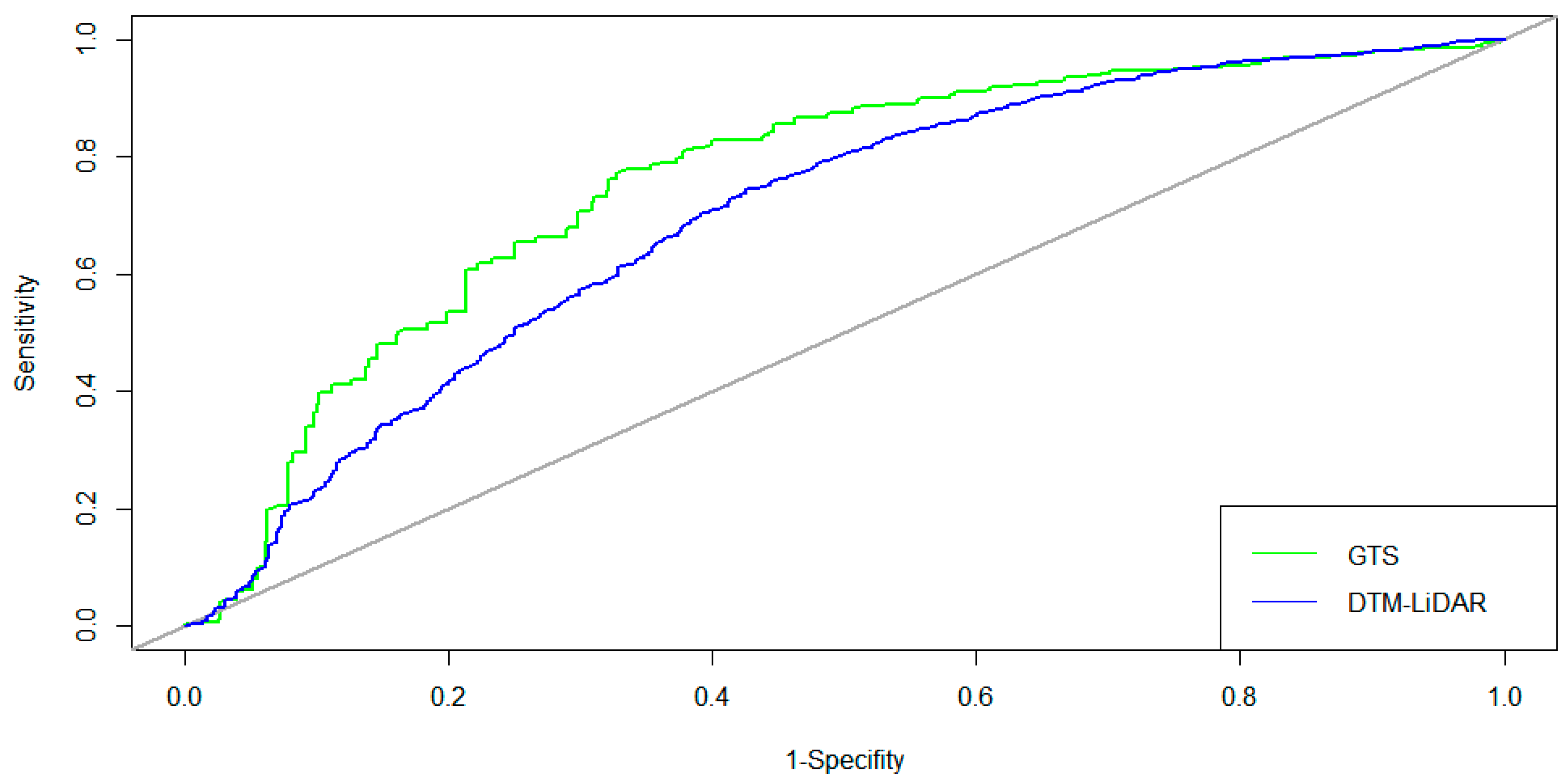
The accuracy of the landslide prediction map produced by the 4SLIDE was evaluated by Relative Operating Characteristics (ROC) analysis [53]. The method provides a curve given by a confusion matrix of binary classification according to four possible outcomes: true positive (TP), true negative (TN), false positive (FP), and false negative (FN). The outcomes are derived by comparing results of the model with the ground truth survey (GTS), which are established by surveys. ROC Curve is a method that compares true positive rates against false positive rates. The Areas Under the Curve (A.U.C., which range from 0.5 to 1.0) are indices of accuracy assessment (Table 4); a nonparametric method for estimating A.U.C. was used for comparing two ROC curves [54]. Statistical analyses were conducted using R software program (www.r-project.org).
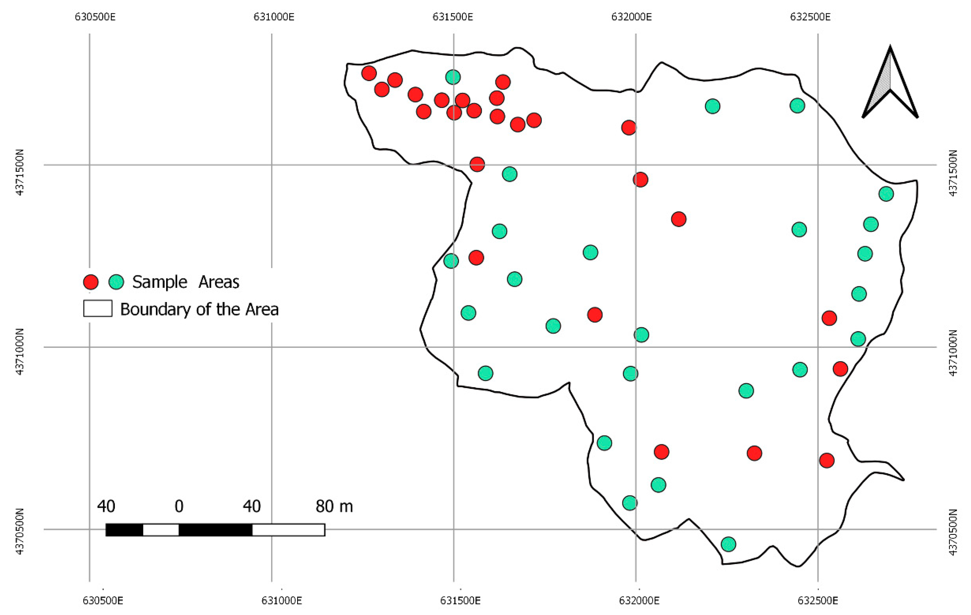
A geomorphology survey is essential to construct the landslide inventory database for defining the accuracy of the landslide prediction map produced by 4SLIDE. For this reason, 50 sample points (Figure 5) within the basin were randomly extracted through GIS, defining the ground-truth survey. For each random point, a sample area of 20 m in diameter was investigated (Figure 6). Each area was surveyed to check for the presence/absence of landslides using two methods. Firstly, GTS that was conducted in August 2017 for the entire basin. Secondly, a DTM was generated from LiDAR point clouds. “Hillshade” viewing allowed visualization of the terrain such that distinct landslide characteristics were identified within the sample areas. The database created included information on the location, dimensions, and other features of landslide occurrence and the locations of non-landslide areas to use these during the training and predictive phases. The database was used also for the ROC analysis. Fifty sample areas (Figure 5) were defined and the two relief methods (GTS and LiDAR data) were superimposed to check for the presence/absence of landslides. Based on this overlap of both relief methods, each pixel was assigned 1 (presence) or 0 (absence) for landslide occurrence.

3. Results

3.1. Performance of 4SLIDE (Calibration/Validation) Using the Physical Similarity Method

The 4SLIDE considers soil features, vegetation effects, and hydraulic factors for determining slope stability. The resulting map is characterized by five stability classes (Figure 6) according to the FS index value (Table 1).
The classification results show that 15% of the study area is classified in the “upper threshold of instability” (0.0 < FS < 0.5), 36% medium susceptibility (0.5 < FS < 1.3), and 20% in low to very low class of stability (FS > 1.3) (Figure 7).
These results highlight that the areas with highest landslide susceptibility are mainly located on steep slopes and unconsolidated lithologies (e.g., colluvial material), which are generally adjacent to the river (Figure 6). In contrast, areas upslope of the stream are generally characterized by low landslide susceptibility.
According to A.U.C. method, the model performance between the GTS and DTM-LiDAR was 0.76 and 0.70, respectively (Figure 8).
These results show that the model has good predictive capability for identifying the areas at risk of shallow landslides and the testing method using DTM-LIDAR data gave similar results compared to GTS. According to the obtained A.U.C. values and classification [54], the model predictive accuracy was assessed as good for both methods. Overall, the result showed good agreement between the susceptibility map and the landslide location data collected in the field. The 4SLIDE, like other predictive models, requires a large amount of information for initialization and parameterization. To further test the effect of the root systems, a simulation with 4SLIDE was performed, eliminating the effect of root cohesion. The main result of this simulation was a greater increase of unstable areas. The new FS index map was reported in Figure 6 and is characterized by five classes (Figure 8) according to the FS index value (Table 1). The classification results show that 6% of the study area is classified in the “upper threshold of instability” (0.0 < FS < 0.5), 40% medium susceptibility (0.5 < FS < 1.3), and 28% in low to very low class of stability (FS > 1.3) (Figure 8). These results highlight that the areas with highest landslide susceptibility are mainly located on steep slopes.
We had tested the 4SLIDE tool’s in the Bonis catchment without the benefit of vegetation. The simulation showed a significant increase in landslide risk areas, not only in the more sloping areas but also in the flat areas (Figure 9).

3.2. Sensitive Parameters and Their Calibration to Simulate Future Hydrogeological Risk

Five cases were simulated and evaluated (Figure 10) forcing the model with five different initialization datasets of model sensitivity analysis.
FS was mainly sensitive to the friction angle, its slope being equal to 0.844 ± 0.005. Soil unit weight was the second most sensitive parameter (mi = 0.242 ± 0.012), followed by soil cohesion (mi = 0.186 ± 0.012) and finally root cohesion (mi = 0.063 ± 0.000) (Table 5).

4. Discussion

Landslides are among the most costly natural hazards, and, although large catastrophic events are rare, small mass movements are very frequent and produce a large amount of economic losses in the long term [1]. Therefore, defining measures to mitigate risks of landslide hazards is an urgent need, since it could have a great impact on current and future societies. In this context, predictive models can highlight areas which are predisposed to landslides and can be useful for preventive actions. In geomorphology, predictive modelling is used to provide relevant and functional information on earth surface processes and landforms throughout extensive areas because of the scarcity of more conventional data surveys [7,55]. Identification of areas at risk of landslide, determination of landslide locations, and assessment of susceptibility play important roles in regional management activities and mitigation measures. In this context, the 4SLIDE model develops landslide susceptibility maps in forest catchments using several parameters among which are root cohesion, soil characteristics, and terrain morphology. In fact, as reported in Formetta [56], the landslide susceptibility evaluation is formed by three main components: (1) hydrological model estimation of soil moisture and water table depth; (2) computing the factor of safety index (FS) based on the infinite slope model; and (3) GIS for visualization and calculation of the outputs. Landslide analyses at different scales can be conducted by different deterministic models [16]. One of the most common is “Distributed Shallow Landslide Analysis Models” (dSLAM), which employs physical numerical variables [16], but some other models (e.g., 4Slide) use the infinite slope stability theory, including TRIGRS, SINMAP, CHASM, and GEOtop-FS [57]. These models are useful for calculating the susceptibility of shallow landslides. The outputs of these models are the water table depth maps and landslide susceptibility maps. But these models have all different features and their own advantages and disadvantages; in fact, some of these are commercial software, and some are simply plug-ins for CAD or GIS software. Independent software like CHASM has an easy interface useful for the final user, while the model script-based ones (e.g., TRIGRS in Fortran) are less user-friendly, and these latter models are often open source licensed. GEOtop is an independent model for investigating landslide prediction using DTMs and geotechnical and moisture parameters [58]. 4SLIDE, like SHALSTAB [59], analyzes landslide susceptibility at the catchment scale and uses steady-state hydrological processes and the infinite slope approach [60], while SINMAP [37], like 4SLIDE, uses numerical parameters and raster-based GIS images.
The 4SLIDE model differs from existing models because it allows for both the use of uniform numerical data throughout the catchment as well as spatially distributed data using raster maps. The latter method facilitates a much more detailed study of the prevention of shallow landslides. The main function of 4SLIDE is to calculate the FS index by analyzing the runoff process using slope values extracted from the DTM. This feature is useful for landslide study over time and over a large area, and 4SLIDE is an open-source model. In addition, the model uses root cohesion as an input parameter and, like the other input data, this parameter can also be spatially distributed allowing for inclusion of a mix of species. Furthermore, the model presents a simple-to-use graphical input interface. 4SLIDE was tested within the Bonis forest catchment where input data could be sampled and spatially represented on raster maps of soil and vegetation data. The model predicted unstable areas adjacent to the stream mainly due to steep terrain and less vegetation cover. Instead, the most stable areas were in zones with gentler slopes and more vegetation cover.
Accuracy assessment showed that the 4SLIDE model estimated the areas susceptible to landslides correctly, as confirmed by both ground surveys and DTM-LiDAR analysis. The performance of the model was evaluated and compared by ROC curves and A.U.C. values. In fact, A.U.C. values showed acceptable results, while the ground-truth sampling method produced slightly better results than the DTM-LiDAR method. The two methods are useful for determination of ground movement and deformation, characteristic of landslide development. In both cases, the performance of the landslide prediction depends on accurate spatial sampling of the ground surface. While both techniques are important, the GTS method can also detect inactive landslides where there are not surface changes; DTM-LIDAR surveys cannot detect this difference [61]. In addition, to test model uncertainty, a sensitivity analysis was performed by varying soil parameters in the ISSE. This analysis showed that a 5 or 10% decrease in the friction angle generates a high increase in slip areas. This is mainly due to the sandy soil that undergoes a greater effect on slope stability by varying the friction angle [7]. Other parameters of the model were much less sensitive to changes. For other soil types, sensitivity results may differ.
4SLIDE accurately determined areas that are susceptible to failure exclusively within the forest basin. The main advantage of the model is the ability to input spatially distributed data, including modifying vegetation cover within the basin and its effects on landslide susceptibility. Such assessments are useful for regional hazard and forest management planning, particularly in cases of removal of forest cover (e.g., fire, large storms, insect outbreaks, poor harvesting, and logging practices). For this reason, a simulation was performed, excluding the contribution of the all vegetation in the Bonis Catchment, which showed a high increase in the areas susceptible to landslides. The new simulation confirmed the importance of vegetation for slope stabilization and how poor forest management can lead to an increase of the susceptibility of landslides.
The main limitation of the model is that it cannot be applied in urban areas, where water drainage structures exist and where buildings and fills may influence slope stability [1]. Another limit of 4SLIDE is that it must interface within commercial GIS software; thus, although the model is freely available, users must have access to the software. Thus, the next steps will be to adapt the model for application in urban areas and utilize an open source software GIS like QGIS.

5. Conclusions

Natural hazards are those processes that occur naturally and when they damage or negatively affect people, property, or the environment, they result in disasters. Natural hazards and associated disasters are of increasing importance in today’s globalized societies. In the 20th century, more than 4.5 million people died and 200 million were damaged by natural hazards. Landslides are one of the costliest risks and although large catastrophic events are rare, small movements are very frequent and produce a large amount of long-term economic losses. As such, it is necessary to develop innovative measures to mitigate risks because of the large impacts they can inflict on society.
Mapping inventories of these phenomena show the spatial attributes of landslides. In geomorphology, predictive modelling of landslides is used to provide relevant and functional information on earth surface process and landforms over extensive areas because these typologies are generally unavailable in conventional surveys [58]. In this study, a theoretical model for shallow landslides was developed and implemented. The 4SLIDE model is based on physical and local parameters, such as slope gradient, lithology, elevation, aspect, root cohesion, and land use/land cover. The model delineates the areas most prone to shallow landslides and is intended to for general planning and rather simple predictive applications. The model predicted spatial landslide occurrence with a moderate level accuracy in our catchment based on two validation methods. As such, the application of this model reduces the difficulties associated with data acquisition in harsh mountainous environments. Of course, better ground-based data will produce more reliable predictions. In terms of practical applications, we note that landslide susceptibility is necessary for a risk assessment and additional efforts should focus on the importance of both natural and urban vegetation and practices for reducing landslide hazards.

Author Contributions

Conceptualization, F.V.M., M.M., and G.S.M.; Methodology, F.V.M.; Software, F.V.M. and M.M.; Validation, F.V.M., M.M., and A.C.; Formal Analysis, F.V.M. and M.M.; Investigation, F.V.M. and M.M.; Resources, G.S.M. and G.M.; Data Curation, F.V.M., M.M., and A.C.; Writing—Original Draft Preparation, F.V.M., M.M., A.C., G.M., G.S.M., and R.C.S.; Writing—Review & Editing, F.V.M., G.S.M., and R.C.S.; Visualization, F.V.M., M.M., and G.S.M.; Supervision, G.S.M.; Project Administration, G.S.M.; Funding Acquisition, G.M. and G.S.M. All authors have read and agreed to the published version of the manuscript.

Funding

This research received no external funding.

Acknowledgments

The study was supported by the research project “ALForLab” (PON03PE_00024_1) co-funded by the (Italian) National Operational Program for Research and Competitiveness (PON R&C) 2007–2013, through the European Regional Development Fund (ERDF) and national financial resources (Revolving Fund—Cohesion Action Plan (CAP) MIUR), by the “Departments of Excellence-2018” Program (Dipartimenti di Eccellenza) of the Italian Ministry of Education, University and Research, DIBAF-Department of University of Tuscia, Project “Landscape 4.0—food, wellbeing and environment” and by the MIUR Research Project of National Relevance (PRIN) Prot. 2015YW8JWA.

Conflicts of Interest

The authors declare no conflict of interest.

Appendix A

Figure A1. Flow chart of model development procedure.
Geosciences 10 00309 g0a1
Figure A2. Dialog box to enter the model parameters.
Geosciences 10 00309 g0a2
Figure A3. Soil sampling points.
Geosciences 10 00309 g0a3
Figure A4. Point cloud of the study area.
Geosciences 10 00309 g0a4
Figure A5. Digital terrain model of the study area.
Geosciences 10 00309 g0a5
Figure A6. Slope map of the study area.
Geosciences 10 00309 g0a6
Figure A7. Groundwater table of the study area.
Geosciences 10 00309 g0a7

References

  1. Sidle, R.C.; Ochiai, H. Natural factors influencing landslides. Landslides Process. Predict. Land Use 2006, 18, 41–119. [Google Scholar] [CrossRef]
  2. Sidle, R.C.; Bogaard, T.A. Dynamic earth system and ecological controls of rainfall-initiated landslides. Earth Sci. Rev. 2016, 159, 275–291. [Google Scholar] [CrossRef]
  3. Sidle, R.C. A theoretical model of the effects of timber harvesting on slope stability. Water Resour. Res. 1992, 28, 1897–1910. [Google Scholar] [CrossRef]
  4. Salvati, P.; Bianchi, C.; Rossi, M.; Guzzetti, F. Societal landslide and flood risk in Italy. Nat. Hazards Earth Syst. Sci. 2010, 10, 465–483. [Google Scholar] [CrossRef]
  5. Trigila, A.; Iadanza, C. Classificazione dei Dissesti e Delle Opere di Difesa del Suolo Nella Banca Dati ReNDiS-Aggiornamento 2013; ISPRA: Roma, Italy, 2013. [Google Scholar]
  6. Trigila, A.; Iadanza, C.; Esposito, C.; Scarascia-Mugnozza, G. Comparison of Logistic Regression and Random Forests Techniques for Shallow Landslide Susceptibility Assessment in Giampilieri (NE Sicily, Italy). Geomorphology 2015, 249, 119–136. [Google Scholar] [CrossRef]
  7. Guha-Sapir, D.; Hoyois, P.; Wallemacq, P.; Below, R. Annual Disaster Statistical Review 2016: The Numbers and Trends; Centre for Research on the Epidemiology of Disasters: Brussels, Belgium, 2016. [Google Scholar]
  8. Guzzetti, F.; Stark, C.P.; Salvati, P. Evaluation of flood and landslide risk to the population of Italy. Environ. Manag. 2005, 36, 15–36. [Google Scholar] [CrossRef] [PubMed]
  9. Spizzichino, D.; Cacace, C.; Iadanza, C.; Trigila, A. Cultural Heritage exposed to landslide and flood risk in Italy. In Proceedings of the EGU General Assembly Conference Abstracts 2013, Vienna, Austria, 7–12 April 2013; Volume 15. [Google Scholar]
  10. Canuti, P.; Casagli, N.; Ermini, L.; Fanti, R.; Farina, P. Landslide activity as a geoindicator in Italy: Significance and new perspectives from remote sensing. Environ. Geol. 2004, 45, 907–919. [Google Scholar] [CrossRef]
  11. Di Lallo, G.; Maesano, M.; Masiero, M.; Mugnozza, G.S.; Marchetti, M. Analyzing strategies to enhance small and low intensity managed forests certification in Europe using SWOT-ANP. Small Scale For. 2016, 15, 393–411. [Google Scholar] [CrossRef]
  12. Frate, L.; Carranza, M.L.; Garfì, V.; Di Febbraro, M.; Tonti, D.; Marchetti, M.; Ottaviano, M.; Santopuoli, G.; Chirici, G. Spatially explicit estimation of forest age by integrating remotely sensed data and inverse yield modeling techniques. IForest 2016, 9, 63–71. [Google Scholar] [CrossRef] [Green Version]
  13. Santopuoli, G.; Di Febbraro, M.; Maesano, M.; Balsi, M.; Marchetti, M.; Lasserre, B. Machine Learning Algorithms to Predict Tree-Related Microhabitats using Airborne Laser Scanning. Remote Sens. 2020, 12, 2142. [Google Scholar] [CrossRef]
  14. Sidle, R.C.; Pearce, A.J.; O’Loughlin, C.L. Hillslope stability and land use. Am. Geophys. Union 1985. [Google Scholar] [CrossRef]
  15. Maesano, M.; Lasserre, B.; Masiero, M.; Tonti, D.; Marchetti, M. First Mapping of the Main High Conservation Value Forests (HCVFs) at National Scale: The Case of Italy. Plant Biosyst. Int. J. Deal. Asp. Plant Biol. 2016, 150, 208–216. [Google Scholar] [CrossRef]
  16. Wu, W.; Sidle, R.C. A distributed slope stability model for steep forested basins. Water Resour. Res. 1995, 31, 2097–2110. [Google Scholar] [CrossRef]
  17. Sidle, R.C.; Wu, W. Simulating effects of timber harvesting on the temporal and spatial distribution of shallow landslides. Z. Geomorphol. 1999, 185–201. [Google Scholar] [CrossRef]
  18. An, K.; Kim, S.; Chae, T.; Park, D. Developing an accessible landslide susceptibility model using open-source resources. Sustainability 2018, 10, 293. [Google Scholar] [CrossRef] [Green Version]
  19. Pal, S.C.; Chowdhuri, I. GIS-based spatial prediction of landslide susceptibility using frequency ratio model of Lachung River basin, North Sikkim, India. SN Appl. Sci. 2019, 1, 416. [Google Scholar] [CrossRef] [Green Version]
  20. Hammond, C.J.; Prellwitz, R.W.; Miller, S.M. Landslide hazard assessment using Monte Carlo simulation. In Proceedings of the 6th International Symposium on Landslides, Christchurch, New Zealand, 10–14 February 1992; Balkema: Amsterdam, The Netherlands; Volume 2, pp. 251–294. [Google Scholar]
  21. Van Western, C.J.; Terlien, T.J. An approach towards deterministic landslide hazard analysis in GIS: A case study from Manizales (Columbia). Earth Surf. Proc. Landf. 1996, 21, 853–868. [Google Scholar] [CrossRef]
  22. Chae, B.-G.; Lee, J.-H.; Park, H.-J.; Choi, J. A method for predicting the factor of safety of an infinite slope based on the depth ratio of the wetting front induced by rainfall infiltration. Nat. Hazards Earth Syst. Sci. 2015, 15, 1835–1849. [Google Scholar] [CrossRef] [Green Version]
  23. Zhao, C.; Lu, Z. Remote sensing of landslides—A review. Remote Sens. 2018, 10, 279. [Google Scholar] [CrossRef] [Green Version]
  24. Wei, C.; Pourghasemi, H.R.; Kornejady, A.; Xie, X. GIS-Based Landslide Susceptibility Evaluation Using Certainty Factor and Index of Entropy Ensembled with Alternating Decision Tree Models; Springer: Cham, Switzerland, 2019; pp. 225–251. [Google Scholar]
  25. Montgomery, D.R.; Dietrich, W.E. A physically based model for the topographic control on shallow landsliding. Water Resour. Res. 1994, 30, 1153–1171. [Google Scholar] [CrossRef]
  26. Beven, K. TOPMODEL: A critique. Hydrol. Process. 1997, 11, 1069–1085. [Google Scholar] [CrossRef]
  27. Wu, T.H.; McKinnell, W.P., III; Swanston, D.N. Strength of tree roots and landslides on Prince of Wales Island, Alaska. Can. Geotech. J. 1979, 16, 19–33. [Google Scholar] [CrossRef]
  28. Sidle, R.C.; Alan, D.; Ziegler, J.N.; Nik, N.R.; Siew, R.; Turkelboom, F. Erosion processes in steep terrain—Truths, myths, and uncertainties related to forest management in Southeast Asia. Forest Ecol. Manag. 2006, 224, 199–225. [Google Scholar] [CrossRef]
  29. Burroughs, B.A.; Hayes, D.B.; Klomp, K.D.; Hansen, J.F.; Mistak, J. Effects of Stronach dam removal on fluvial geomorphology in the Pine River, Michigan, United States. Geomorphology 2009, 110, 96–107. [Google Scholar] [CrossRef]
  30. Sidle, R.C.; Swanston, D.N. Analysis of a small debris slide in coastal Alaska. Can. Geotech. J. 1982, 19, 167–174. [Google Scholar] [CrossRef]
  31. Beven, K.; Freer, J. A dynamic topmodel. Hydrol. Process. 2001, 15, 1993–2011. [Google Scholar] [CrossRef]
  32. Beven, K.J.; Kirkby, M.J.; Schofield, N.; Tagg, A.F. Testing a physically-based flood forecasting model (TOPMODEL) for three UK catchments. J. Hydrol. 1984, 69, 119–143. [Google Scholar] [CrossRef]
  33. Kirkby, M.J.; Statham, I. Surface stone movement and scree formation. J. Geol. 1975, 83, 349–362. [Google Scholar] [CrossRef]
  34. Abernethy, B.; Rutherfurd, I.D. The distribution and strength of riparian tree roots in relation to riverbank reinforcement. Hydrol. Process. 2001, 15, 63–79. [Google Scholar] [CrossRef]
  35. Genet, M.; Stokes, A.; Salin, F.; Mickovski, S.B.; Fourcaud, T.; Dumail, J.F.; Van Beek, R. The influence of cellulose content on tensile strength in tree roots. Plant Soil 2005, 278, 1–9. [Google Scholar] [CrossRef]
  36. Moresi, F.V.; Maesano, M.; Matteucci, G.; Romagnoli, M.; Sidle, R.C.; Mugnozza, S.G. Root Biomechanical Traits in a Montane Mediterranean Forest Watershed: Variations with Species Diversity and Soil Depth. Forests 2019, 10, 341. [Google Scholar] [CrossRef] [Green Version]
  37. Pack, R.T.; Tarboton, D.G.; Goodwin, C.N. The SINMAP approach to terrain stability mapping. In Proceedings of the 8th Congress of the International Association of Engineering Geology, Vancouver, BC, Canada, 21–25 September 1998; Volume 21, p. 25. [Google Scholar]
  38. Guzzetti, F. Landslide fatalities and the evaluation of landslide risk in Italy. Eng. Geol. 2000, 58, 89–107. [Google Scholar] [CrossRef]
  39. Conforti, M.; Pascale, S.; Robustelli, G.; Sdao, F. Evaluation of prediction capability of the artificial neural networks for mapping landslide susceptibility in the Turbolo River catchment (northern Calabria, Italy). Catena 2014, 113, 236–250. [Google Scholar] [CrossRef]
  40. Brunori, E.; Maesano, M.; Moresi, F.V.; Matteucci, G.; Biasi, R.; Mugnozza, S.G. The hidden land conservation benefits of olive-based (Olea europaea L.) landscapes: An agroforestry investigation in the southern Mediterranean (Calabria region, Italy). Land Degrad. Dev. 2020, 31, 801–815. [Google Scholar] [CrossRef]
  41. Iovine, G.G.R.; Gariano, S.L.; Iaquinta, P.; Lollino, P.; Terranova, O.G. Limit Equilibrium Analysis and Real-Time Monitoring as Support for Landslide Risk Mitigation: The San Rocco Case Study at San Benedetto Ullano (Calabria). Disaster Manag. Earth Obs. 2011. [Google Scholar] [CrossRef] [Green Version]
  42. Collalti, A.; Biondo, C.; Buttafuoco, G.; Maesano, M.; Caloiero, T.; Lucà, F.; Pellicone, G.; Ricca, N.; Salvati, R.; Veltri, A.; et al. Simulation, calibration and validation protocols for the model 3D-CMCC-CNR-FEM: A case study in the Bonis’ watershed (Calabria, Italy). Forest 2017, 14, 247–256. [Google Scholar] [CrossRef] [Green Version]
  43. Bonardi, G.; Cavazza, W.; Perrone, V.; Rossi, S. Calabria-Peloritani terrane and northern Ionian sea. In Anatomy of an Orogen: The Apennines and Adjacent Mediterranean Basins; Springer: Dordrecht, The Netherlands, 2001; pp. 287–306. [Google Scholar] [CrossRef]
  44. Bonardi, G.; Capoa, P.D.; Staso, A.D.; Perrone, V.; Sonnino, M.; Tramontana, M. The age of the Paludi Formation: A major constraint to the beginning of the Apulia-verging orogenic transport in the northern sector of the Calabria–Peloritani Arc. Terra Nova 2005, 17, 331–337. [Google Scholar] [CrossRef]
  45. Barone, M.; Dominici, R.; Muto, F.; Critelli, S. Detrital modes in a late Miocene wedge-top basin, northeastern Calabria, Italy: Compositional record of wedge-top partitioning. J. Sediment. Res. 2008, 78, 693–711. [Google Scholar] [CrossRef]
  46. Corbi, F.; Fubelli, G.; Lucà, F.; Muto, F.; Pelle, T.; Robustelli, G.; Scarciglia, F.; Dramis, F. Vertical movements in the Ionian margin of the Sila Massif (Calabria, Italy). Ital. J. Geosci. 2009, 128, 731–738. [Google Scholar] [CrossRef]
  47. Raab, G.; Halpern, D.; Scarciglia, F.; Raimondi, S.; Norton, K.; Pettke, T.; Hermann, J.; de Castro Portes, R.; Sanchez, A.M.A.; Egli, M. Linking tephrochronology and soil characteristics in the Sila and Nebrodi mountains, Italy. Catena 2017, 158, 266–285. [Google Scholar] [CrossRef]
  48. Conforti, M.; Lucà, F.; Scarciglia, F.; Matteucci, G.; Buttafuoco, G. Soil carbon stock in relation to soil properties and landscape position in a forest ecosystem of southern Italy (Calabria region). Catena 2016, 144, 23–33. [Google Scholar] [CrossRef]
  49. Callegari, G.; Ferrari, E.; Garfiz, G.; Iovino, F.; Veltri, A. Impact of thinning on the water balance of a catchment in a Mediterranean environment. For. Chron. 2003, 79, 301–306. [Google Scholar] [CrossRef]
  50. Bellotti, R.; Selleri, G. Correlazione tra le caratteristiche geotecniche di alcuni terreni di fondazione e confronto tra i risultati ottenibili con l’applicazione di diversi metodi di calcolo del carico ammissibile. Riv. Ital. Geotec. 1969, 2, 95–103. [Google Scholar]
  51. Morris, M.D. Factorial sampling plans for preliminary computational experiments. Technometrics 1991, 33, 161–174. [Google Scholar] [CrossRef]
  52. Collalti, A.; Thornton, P.E.; Cescatti, A.; Rita, A.; Nolè, A.; Borghetti, M.; Trotta, C.; Ciais, P.; Matteucci, G. The sensitivity of the forest carbon budget shifts between different parameters and processes along stand development and climate change. Ecol. Appl. 2019, 29, e01837. [Google Scholar] [CrossRef] [PubMed] [Green Version]
  53. Rossi, L.M.; Rapidel, B.; Roupsard, O.; Villatoro-Sánchez, M.; Mao, Z.; Nespoulous, J.; Perez, J.; Prieto, I.; Roumet, C.; Metselaar, K.; et al. Sensitivity of the landslide model LAPSUS_LS to vegetation and soil parameters. Ecol. Eng. 2017, 109, 249–255. [Google Scholar] [CrossRef]
  54. Fawcett, T. An introduction to ROC analysis. Pattern Recognit. Lett. 2006, 27, 861–874. [Google Scholar] [CrossRef]
  55. DeLong, E.R.; DeLong, D.M.; Clarke-Pearson, D.L. Comparing the areas under two or more correlated receiver operating characteristic curves: A non-parametric approach. Biometrics 1988, 44, 837–845. [Google Scholar] [CrossRef]
  56. Formetta, G.; Rago, V.; Capparelli, G.; Rigon, R.; Muto, F.; Versace, P. Integrated physically based system for modeling landslide susceptibility. Procedia Earth Planet. Sci. 2014, 9, 74–82. [Google Scholar] [CrossRef] [Green Version]
  57. Nilsson, B.; Højberg, A.L.; Refsgaard, J.C.; Troldborg, L. Uncertainty in geological and hydrogeological data. Hydrol. Earth Syst. Sci. Discuss. 2006, 3, 2675–2706. [Google Scholar] [CrossRef] [Green Version]
  58. Vieira, B.C.; Fernandes, N.F. Shallow landslide prediction in the Serra do Mar, São Paulo, Brazil. Nat. Hazards Earth Syst. Sci. 2010, 10, 1829–1837. [Google Scholar] [CrossRef]
  59. Dietrich, W.; Montgomery, D. A Digital Terrain Model for Mapping Shallow Landslide Potential (SHALSTAB); University of California: Berkeley, CA, USA, 1988. [Google Scholar]
  60. Martínez-Graña, A.M.; Goy, J.L.; Zazo, C. Geomorphological applications for susceptibility mapping of landslides in natural parks. Environ. Eng. Manag. J. (EEMJ) 2009, 15, 327–338. [Google Scholar] [CrossRef]
  61. Toth, C.K.; Mora, O.E.; Lenzano, M.G.; Grejner-Brzezinska, D.A.; Beach, K. Landslide hazard detection from LiDAR data. In Proceedings of the ASPRS 2013 Annual Conference, Baltimore, MD, USA, 26–28 March 2013; pp. 24–28. [Google Scholar]
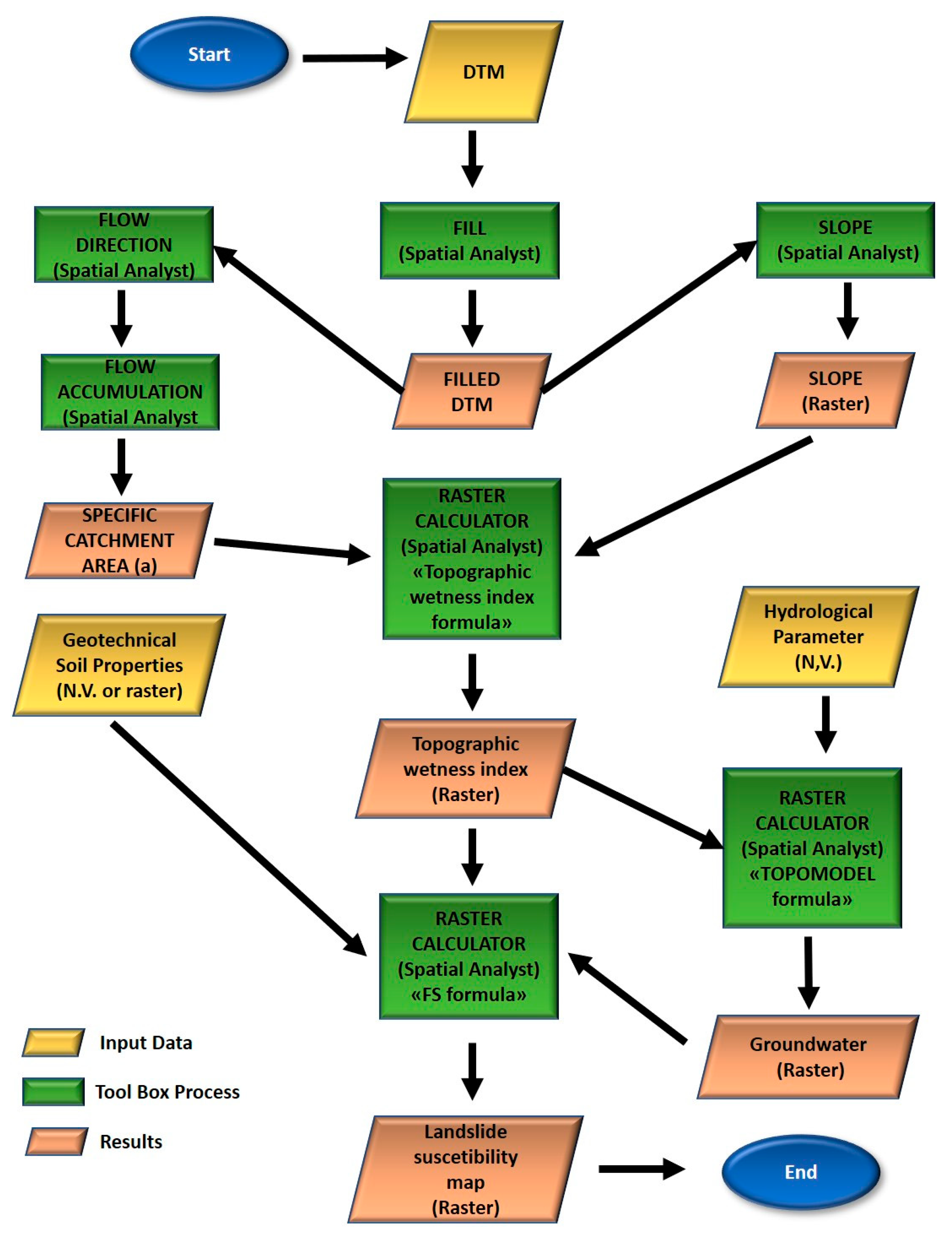
Figure 1. Data processing workflow as implemented in the Model Builder application.
Geosciences 10 00309 g001
Figure 2. Study area, the watershed of Bonis.
Geosciences 10 00309 g002
Figure 3. Land cover map of the Bonis catchment.
Geosciences 10 00309 g003
Figure 4. Soil map of the Bonis catchment.
Geosciences 10 00309 g004
Figure 5. Sample plots randomly distributed within the study area Green areas are not subject to landslides; those in red are subject to landslides.
Geosciences 10 00309 g005
Figure 6. Map of landslide susceptibility based on the model.
Geosciences 10 00309 g006
Figure 7. Percentages of catchment area partitioned in five categories of landslide susceptibility based on modelling results.
Geosciences 10 00309 g007
Figure 8. Relative Operating Characteristics (ROC) curve for the landslide prediction map based on the model.
Geosciences 10 00309 g008
Figure 9. Map of landslide susceptibility without benefit of the vegetation.
Geosciences 10 00309 g009
Figure 10. Sensitivity analysis for the five input parameters.
Geosciences 10 00309 g010
Table 1. FS value classes in the map.
Predicted Stability ZoneRelative Slide RankingFactor of Safety Index (FS)
Upper Threshold of InstabilityHigh0 < FS ≤ 0.5
Lower Threshold of InstabilityModerate0.5 < FS ≤ 1
Nominally StableLow1 < FS ≤ 1.3
Moderately StableVery Low1.3 < FS ≤ 1.50
StableStableFS > 1.50
Table 2. Model data input.
Input ParametersDescriptionNumerical Value/Input Type Data
Cell Size (m)Size of the cell sideN.V.
Transmissivity (m2/h)Transmissivity: the rate at which groundwater flows horizontally through an aquifer.N.V./raster map
Effective Drainable PorosityPorosity: a measure of the void spaces in a material quantified as the fraction of the volume of voids per unit volume. N.V./raster map
Basin Area (m2)A drainage basin or catchment basin is the area of land where all surface water converges to a single point at a lower elevation, usually the outlet of the basin.N.V.
Flow at the Watershed Outlet (m3/s)The flow rate is the amount of water that crosses a channel cross-section of area A per unit time. N.V./raster map
Input Raster DTMDigital terrain model (DTM) is a 3D representation of the terrain surface. Raster DTM
Root Cohesion (kPa)Root systems contribute to soil strength by providing an artificial cohesion that can be added to effective soil cohesion in the Mohr-Couloumb equation for shear strength.N.V./raster map
Cohesion (kPa)Soil cohesion is the inherent “stickiness” of the material, caused by the attraction of its molecules to each other. For example, clay soils are cohesive, while dry sand is non-cohesive.N.V./raster map
Internal Angle Of Friction (Rad)Soil friction angle is a parameter related to shear strength of soils. It is experimentally derived from Mohr-Coulomb failure criterion and is used to describe the frictional shear resistance of soil grains together with the normal effective stress.N.V./raster map
Weight of Saturated Soil (kg/cm3)Moist unit weight, which is the unit weight of a soil when all void spaces are filled with water.N.V./raster map
Soil Depth (m)Soil depth is the vertical soil thickness.N.V./raster map
Weight of Soil (kg/cm3)Dry unit weight is the unit weight of a soil when all void spaces of the soil are completely filled with air.N.V./raster map
Table 3. Geotechnical parameters of the study area.
LithologyCohesion
(kPa)
Internal Friction Angle
(rad)
Unit Weight of Soil
(kN/m3)
Unit Weight of Saturated Soil
(kN/m3)
Hydraulic Conductivity
m2/h
Clay and sand13.720.3715.319.20.172
Clay20.300.3413.618.50.072
Sand00.6113.416.90.802
Sand and Silt8.160.5214.818.80.680
Silt12.740.4216.620.60.502
Table 4. Values proposed by Landis and Koch (1977).
Area under the ROC CurveValidation
A.U.C. ≤ 0.5Poor
0.5 < A.U.C. < 0.7Slight
0.7 < A.U.C. ≤ 0.9Fair
0.9 < A.U.C. < 1.0Moderate
A.U.C. = 1.0Perfect
Table 5. Results of the simulations performed for different input parameters.
Input ParameterPercentage VariationMean FSFS MaxFS MinPercentage Variationmi
Cohesion101.67284.030.142.1580.192454858
51.68280.320.140.823
−51.65275.570.14−0.886
−101.64273.460.13−1.646
Friction Angle101.81301.810.248.5510.083363123
51.74289.840.234.245
−51.60266.390.22−4.188
−101.53254.890.21−8.322
Root Cohesion103.25279.790.220.6336.7987 × 10−17
51.67278.910.220.316
−53.22277.150.14−0.316
−103.21276.270.14−0.633
Soil Unit Weight101.69285.480.212.6780.1860320961
51.66281.550.221.265
−51.65274.870.23−1.138
−101.64272.010.24−2.168
Water Unit Weight101.67278.030.22−0.0024.25108 × 10−6
51.67278.030.22−0.001
−51.67278.040.220.001
−101.67278.040.220.002