Assessing the Frequency of Floods in Ice-Covered Rivers under a Changing Climate: Review of Methodology

Abstract

Ice-influenced hydrologic and hydrodynamic processes often cause floods in cold regions of the globe. These floods are typically associated with ice jams and can have negative socio-economic impacts, while their impacts on riverine ecosystems can be both detrimental and beneficial. Several methods have been proposed for constructing frequency distributions of ice-influenced annual peak stages where historical data are scarce, or for estimating future frequencies under different climate change scenarios. Such methods rely on historical discharge data, which are generally easier to obtain than peak stages. Future discharges can be simulated via hydrological models, driven by climate-model output. Binary sequences of historical flood/no-flood occurrences have been studied using logistic regression on physics-based explanatory variables or exclusively weather-controlled proxies, bypassing the hydrological modelling step in climate change projections. Herein, background material on relevant river ice processes is presented first, followed by descriptions of various proposed methods to quantify flood risk and assess their advantages and disadvantages. Discharge-based methods are more rigorous; however, projections of future flood risk can benefit from improved hydrological simulations of winter and spring discharges. The more convenient proxy-based regressions may not adequately reflect the controlling physics-based variables, while extrapolation of regression results to altered climatic conditions entails further uncertainty.

1. Introduction

River ice processes in general and ice jams, in particular, are actively studied in Asia, Europe, and North America, as can be seen in various publications, such as [1,2,3,4,5,6,7,8,9,10,11]. Recognizing the importance of ice to a large portion of the globe, the International Association for Hydro-Environment Engineering and Research (IAHR) sponsors biennial Ice Symposia, where scientists from many nations present and discuss new results; their contributions can be found in the proceedings of each symposium.

Floods in cold regions of the globe can be caused by both open water and ice-influenced hydrologic and hydrodynamic processes. Ice-related floods are typically associated with the formation or release of ice jams, which often dominate the frequency of extreme water stages and associated flood damages (see, for example, major ice jam occurrences and impacts in Asia, Europe, and North America in [12]). Ice jam floods have negative socio-economic impacts (e.g., mass evacuation, loss of human life, damage to property and infrastructure) while their effects on riverine ecosystems can be both detrimental (e.g., fish mortality, loss of spawning grounds) and beneficial (e.g., replenishment of floodplain ecosystems with river water, sediment, and nutrients). For detailed information on the socio-economic and ecological impacts of ice jams, see, for example [13,14,15,16,17].

Assessing the frequency and damage potential of ice jam floods (IJFs) is an essential step in regulating floodplain development, identifying effective ice jam mitigation measures, and anticipating the impacts of building new in-river structures or removing old ones. The same applies to assessing the positive or negative ecological implications of river regulation or of climate change [18]. As with open water flooding, IJF recurrence and damage potential at a particular location are quantified by developing a stage-frequency relationship and coupling it with an independently obtained relationship between stage and cost of flood damage. The stage-frequency relationship, which is controlled by river ice processes, forms the subject of this review.

Several characteristics of ice events render them less than amenable to traditional stage-frequency analyses. The complex hydrometeorological and structural processes that lead to ice jam formation, progression, and release are highly site-specific. Therefore, regional parametric equations, such as those developed for open water flood frequency studies, do not apply. Moreover, historical data gaps are much more frequent for ice-related events because ice often damages hydrometric gauges (Figure 1), usually when an ice jam forms nearby. Not only does this cause the ice-influenced historical stage record to be shorter than the open water record, but the missing data are also often associated with extreme events.

Four different approaches for developing stage-frequency distributions of ice-related events have been identified [19]. The biophysical approach uses physical characteristics (e.g., vegetation, soils, debris lines) of topography and ecology to identify high water levels and flood extent areas. The historical flood approach utilizes field (e.g., high-water marks) and photographic (aerial photo, satellite imagery) information, while the flood-envelope approach involves data from multiple past flood events. The hydrotechnical approach is based on hydraulic or hydrodynamic models and is suited for situations in which information on past flood stages is limited. In such instances, the available information is used to calibrate an analytical or numerical model that links ice jam stage to river discharge. The latter is a variable that is much more readily available than ice jam stage [20,21]. Once the model is calibrated, it can be applied to all years of record to synthetically reconstruct annual values of peak ice-influenced stages.

It is only the hydrotechnical, from among these four approaches, that can furnish projections to future IJF frequency under a changing climate. Such applications link a river ice model to discharges obtained from a hydrologic model, which in turn is driven by projections of climatic variables supplied by various Global or Regional Climate Models (GCM, RCM) under different climate scenarios. An alternative to hydrotechnical modelling for IJF frequency projections is the use of weather-related proxies for relevant hydroclimatic controls [22], bypassing the need for a hydrological model [23].

The objective of this paper is to critically review various methods that can furnish stage-frequency distributions (SFD) for, or flooding potential of, ice-influenced water levels, and thence provide projections of IJF frequency to future years under a changing climate. An overview of the physical processes that generate high water levels during the ice season is presented in the next section. The subsequent five sections describe various methods of developing SFDs for ice-influenced water levels or assessing probabilities of binary occurrences of flood/no flood events. Applications of these methods to future climatic conditions are discussed next, with emphasis on their advantages and disadvantages, as well as on research needs.

2. Physics of Peak River Stages under Ice Conditions

The presence of a floating ice cover in a river enhances the hydraulic resistance to flow by introducing an additional boundary and occupying a portion of the cross-sectional area to accommodate the keel of the floating cover. Where there are no controls on the water level, as is typically the case, these effects result in increased water depths to allow passage of the river discharge. Where artificial or natural controls constrain water level adjustment, rivers respond by reducing their discharge (e.g., Great Lakes connecting channels). A limited local rise in water level may be possible depending on the proximity of the upstream control, but flooding, if any, can be subdued. Considering the added complexity introduced by the controls, this topic is not discussed further herein, beyond stating that it can best be studied with advanced river ice models [24].

The effect of an ice cover on stage is called “backwater”, and is defined as the difference between the ice-influenced water level and the water level that would prevail with the same discharge under open water conditions. This definition applies to steady state or gradually-varied-flow conditions, under which the water surface slope remains constant or almost constant, respectively. In addition to channel bathymetry, slope, and discharge, backwater magnitude is determined by the thickness and underside roughness of the ice cover.

The following relationship illustrates how the channel (mean) depth increases under an ice cover to pass the discharge [25]:

$$\frac{{\mathrm{Y}}_{\mathrm{cov}}}{{\mathrm{Y}}_{\mathrm{op}}}\approx {\left[1+{\left(\frac{{\mathrm{n}}_{\mathrm{i}}}{{\mathrm{n}}_{\mathrm{b}}}\right)}^{\frac{3}{2}}\right]}^{\frac{2}{5}}+0.92\frac{\mathrm{h}}{{\mathrm{Y}}_{\mathrm{op}}}$$

(1)

in which Y denotes depth and the suffixes “cov” and “op” signify ice covered and open water conditions, respectively; h is the aggregate thickness of the ice cover; n_i and n_b denote Manning roughness coefficients for the bottom of the ice cover and the riverbed, respectively. The first term on the right-hand side of Equation (1) is the ratio of the under-ice depth of flow to Y_op, while the second term is the ratio of the keel of the cover (assumed ~0.92 h) to Y_op. For a sheet-ice cover that is as rough as the riverbed, the flow-depth ratio is ~1.3; addition of the keel ratio (~0.1 to 0.2) suggests that the total water depth may be as much as 50% greater than the open water depth at the same discharge.

On the other hand, ice jams can have n_i values two to three times as much as those of typical riverbeds, and an aggregate thickness comparable to or even greater than Y_op. Consequently, jams can easily double the open water depth required to pass the same discharge. When the latter is relatively large, as in unregulated rivers during the breakup period, the backwater can amount to several or many metres, depending on basin hydrology and channel morphology. Backwaters of up to 20 m have been recorded on the Lena River in Siberia, Russia [26].

Apart from complexities caused by dynamic phenomena or by hanging dams, the peak stage occurring in any one ice season ranges between those generated by sheet ice cover and a fully developed or “equilibrium” jam [3], as illustrated in Figure 2. Data points located beneath the calculated sheet ice cover line likely reflect situations in which the peak stage occurred while the ice cover had largely melted away. The data point located above the equilibrium-jam line likely reflects imperfections in the theoretical calculation of ice jam stages for that site. Intermediate data points highlight the fact that equilibrium jams may or may not form at all, or perhaps they are located too far from the gauge site. An individual data point could also be due to the passage of a “jave”, a sharp wave generated by the abrupt release of an upstream ice jam.

The sheet ice and ice jam “envelope” lines shown in Figure 2 can readily be calculated if local channel bathymetry and slope are known, using either analytical or numerical techniques [3,28,29]. The various ways in which an ice jam may affect the peak water level at a specific river site, say a gauge site, are illustrated in Figure 3 and described below.

Case 1: a jam is located far downstream of the gauge site; peak stage = open-water stage, no backwater.

Case 2: jam located downstream of, but not far from, the gauge site; peak stage < equilibrium jam stage.

Case 3: jam fully affects the gauge site; peak stage ≤ equilibrium jam stage. Depending on the volume of available ice rubble, a jam may be too short to attain the equilibrium condition; in that case, it will not match the full jam effect, even when the gauge is located within the main body of the jam.

Case 4: jam is located upstream of gauge site: peak stage = peak of the jave generated upon jam release. The height of a jave is related to, and smaller than, the difference between the total water depths caused by the parent jam and the (usually) ice-covered or open water flow downstream of the toe [30,31]. In turn, this difference increases with increasing discharge and is enhanced by channel width and slope [3]. Ordinarily, the jammed reach upstream of a gauge would be of similar width and slope, so that the jave height will be less than the pre-release difference in depths. Therefore, the peak stage at the gauge will be less than the equilibrium jam stage. However, there is no guarantee that this will always be the case; upstream channel morphology should always be carefully examined, and potential jave heights at the gauge estimated analytically or modeled, as the situation may warrant.

The jams primarily discussed herein are of the so-called “wide-channel” variety [32]. They form by the collapse and shoving of surface accumulations of ice blocks or ice pans, and attain an aggregate thickness that is just adequate to withstand the applied external forces. These forces arise from the flow shear stress exerted at the underside of the jam and from the downslope component of the jam′s own weight; they are resisted by the internal strength of the rubble that comprises the jam, which is generated by the thickness-dependent net buoyancy of the ice accumulation.

In the vast majority of cases, the annual peak ice-influenced water level occurs during the breakup event. Consequently, our narrative will focus on breakup jams, but it should be understood to also apply to freezeup jams that form by the same force balance that controls the thickness of breakup jams. In northern regions, river ice breakup is typically triggered by the early spring freshet, which is driven by snowmelt, possibly augmented by rainfall. At more moderate latitudes and in milder winter regimes, mid-winter breakup events are common because of brief thaws accompanied by rainfall. The resulting runoff is often large enough to initiate breakup, followed by renewed freezeup when the cold weather resumes. Mid-winter jams can be even more extreme than spring jams [33]. Owing to larger natural discharges, breakup jams typically have greater flooding potential than freezeup ones, but freezeup jams can also cause problems [34], especially in regulated rivers where hydropower generation results in much higher, than pristine, discharges [35,36,37].

Less frequently, a damaging ice jam may be of the “hanging dam” variety, which is an accumulation that forms by transport and deposition of frazil slush and ice fragments under an existing ice cover. Typically, the source of ice inflow is a steep reach, occasionally containing rapids, that remains open for a good part of, or for the entire winter. A milder slope farther downstream results in early formation of a sheet ice cover, which provides the platform for deposition of the incoming ice. Hanging dams are too thick to shove and sometimes attain extreme dimensions (e.g., [38]) in deep river sections. Consequently, they could cause the seasonal peak water level in reaches where no wide-channel jams form or in rivers regulated for hydropower generation, where freezeup and winter discharges may be comparable to, or even exceed, breakup discharges. The peak water level caused by a hanging dam during an ice season is not as simply related to discharge as in the case of the wide-channel jam (Figure 2). It depends on various additional factors, such as the upstream supply and properties of frazil ice, which vary with weather conditions and with the length of the frazil-generating open reach upstream of the hanging dam. Comprehensive bibliography on hanging dams and detailed discussion of relevant physical processes is presented in [39].

Overbank flooding may also occur by different mechanisms in small, steep rivers, such as aufeis buildup or bottom-fast ice dams created by anchor ice growth [40,41]. Though not discussed herein, such ice-induced flooding mechanisms should be considered when dealing with small and steep streams.

Where time series of open-water and ice-influenced annual peaks are available, they can be ranked, and respective frequency curves developed using one of several plotting formulae that have been proposed by statisticians. An example is shown in Figure 4, which suggests that ice jams can cause much higher peaks than open-water floods with return periods of ~10 years or more at that particular location. This is common in Canada, though the percentage of river sites at which ice dominates the low-frequency floods has not yet been quantified.

With the open water and ice-influenced SFDs at hand, the combined probability of one or both of the two peaks exceeding any given stage in any given year can be calculated as:

$$\mathrm{P}\left(\mathrm{H}\right)={\mathrm{P}}_{\mathrm{i}}+{\mathrm{P}}_{\mathrm{o}}-{\mathrm{P}}_{\mathrm{i}}{\mathrm{P}}_{\mathrm{o}}$$

(2)

in which H = stage; P(H) = probability that H will be exceeded in any one year, either by an ice-influenced peak or by open-water flooding, or both; and P_i, P_o are exceedance probabilities of ice-influenced peaks and open-water peaks, respectively. Methods to determine P_i are described in the following three sections.

3. Discrete-Outcomes Method

As noted earlier, data on ice-influenced peaks are often so scarce that a hydrotechnical method must be applied to determine the function P_i(H). To my knowledge, the first and simplest such method was proposed in [42] and later amplified in [43]. For brevity, this method is labeled herein the G-C method. The exceedance probability, P_J(H), of an ice-jam stage, H, during any one ice season can be calculated as:

$${\mathrm{P}}_{\mathrm{J}}\left(\mathrm{H}\right)=\mathrm{P}\left({\mathrm{Q}}_{\mathrm{H},\mathrm{J}}\right)\mathrm{P}\left(\mathrm{J}\right)$$

(3)

in which P(Q_H,_J) is the exceedance probability of the discharge (Q_H,J) that corresponds to H under ice-jam conditions (Figure 2); and P(J) is the probability of a jam occurring near the site of interest in any one year. The combined probability, P_i(H), for the ice-influenced stage under both jam and no-jam conditions (mutually exclusive events) is obtained from:

$${\mathrm{P}}_{\mathrm{i}}\left(\mathrm{H}\right)=\mathrm{P}\left({\mathrm{Q}}_{\mathrm{H},\mathrm{J}}\right)\mathrm{P}\left(\mathrm{J}\right)+\mathrm{P}\left({\mathrm{Q}}_{\mathrm{H},\mathrm{NJ}}\right)\mathrm{P}\left(\mathrm{NJ}\right)$$

(4)

in which the suffix NJ denotes the “no-jam” condition. Here, Q_H,NJ is the discharge corresponding to H under the sheet ice condition in Figure 2. Assuming the frequency distribution of breakup discharges is known, the only unknown in Equation (4) will be the probability of jam occurrence, since P(NJ) = 1 − P(J). The parameter P(J) can be calibrated by matching computed SFDs to the known SFDs, which are based on historical water levels. Even where no historical stage data are available, P(J) could be estimated from non-instrumental evidence, such as resident recollections, newspaper reports, etc. (Caution: it may not be possible to obtain a good match between computed and historical SFDs using a single value of P(J), as found in [20] on a few occasions. One could then try a variable, discharge-dependent P(J), or simply adopt a different method).

Uncertainty can be explored by working out scenarios using different P(J) values. As noted earlier, the sheet ice and ice jam envelope lines (Figure 2) can be determined using well-established analytical and numerical modelling applications, after surveying local channel bathymetry and slope. The word “local” here denotes a reach centered at the site of interest and long enough (e.g., ~10 channel widths) to capture average hydraulic characteristics that influence stage-discharge relationships under different flow conditions.

Empirical site-specific evidence may suggest that jams are unstable at very high discharges or may not form at all. This effect can be taken into account by specifying a jam-clearing discharge threshold [44] based on local observations and experience. Moreover, the floodplain configuration may be such that there is a ceiling to how high the water level can rise, owing to spillage and overbank flow, even if ice jams remain in place at very high discharges. This eventuality can only be assessed by experienced professionals, based on careful inspection of the site of interest.

The G-C method assumes discrete outcomes for any given breakup discharge: the annual ice-influenced peak can only take on one of two values (ice jam stage and sheet ice cover stage, per Figure 2). Though unrealistic, this assumption led to a very simple algorithm that triggered various advances in later years. To partially account for peak water levels that are intermediate between the two envelope curves of Figure 2, a second empirical probability is sometimes introduced, that of the peak ice-influenced stage being caused by a jave (case 4 in Figure 3), as outlined in [45,46]. Sophisticated Monte Carlo techniques can also be applied to generate long (e.g., 1000 years) records of “expected” peak ice-influenced stages using the known probability distribution of breakup discharges and the estimated or assumed jam-jave probabilities.

4. Distributed-Outcomes Method

Recognizing that any stage within the envelope lines of Figure 3 (sheet ice cover, ice jam) is possible, Ref. [20] developed the Distributed Function Method (DFM), which considers the probability of peak stage distribution as a function of the prevailing discharge. The DFM makes no assumption as to the cause of the peak stage, but relies on an empirically-established similarity function, φ(η), which describes the conditional non-exceedance probability of the maximum breakup stage, given the value of the breakup discharge:

$$\begin{gathered} \mathrm{P}\{({\mathrm{H}}_{\mathrm{m}}<\mathrm{H})/(\mathrm{Q}<{\mathrm{Q}}_{\mathrm{m}}<\mathrm{Q}+\mathrm{dQ})\}=\mathrm{P}({\mathsf{\eta }}_{\mathrm{m}}<\mathsf{\eta })\equiv \varphi \left(\mathsf{\eta }\right) \\ \mathrm{with}\mathsf{\eta }=\frac{\mathrm{H}-{\mathrm{H}}_{\min }}{\mathrm{H}-{\mathrm{H}}_{\max }} \end{gathered}$$

(5)

in which H_max and H_min are the upper- and lower-envelope stages for the discharge Q_m; and η is the similarity variable. After some algebra, it can be shown that the probability P_i,n (now defined as a non-exceedance probability) is simply given by

$${\mathrm{P}}_{\mathrm{i},\mathrm{n}}=\mathrm{P}\left({\mathrm{H}}_{\mathrm{m}}<\mathrm{H}\right)={{\displaystyle \int }}_0^1\mathsf{\varphi }\left(\mathsf{\eta }\right){\mathrm{dP}}_{\mathrm{Q}}$$

(6)

in which P_Q is the non-exceedance probability of the discharge Q and dP_Q is a small increment of this probability. Data from four Canadian river sites have indicated that the similarity function can be expressed as

$$\mathsf{\varphi }\left(\mathsf{\eta }\right)=\left(\mathrm{k}+1\right)\mathsf{\eta }-{\mathrm{k}\mathsf{\eta }}^2$$

(7)

in which the coefficient k varies from one river site to another; the lower the k value, the more prone a site is to ice-jamming [20]. The form of Equation (7) satisfies the end conditions ϕ(0) = 0, ϕ(1) = 1 and increases monotonically with η for all values of k within the interval [−1, 1]. If k < −1 or if k > 1, Equation (7) will respectively produce negative values or exceed 1 (meaningless outcomes for a probability distribution).

It is not known whether the functional form of Equation (7) applies to all river sites; where it does not, alternative formulations can be used to facilitate the derivation of the local SFD. A form that allows greater flexibility in fitting empirical distributions of the dimensionless variable, η, reads:

$$\mathsf{\varphi }\left(\mathsf{\eta }\right)=\left(\mathrm{s}+1\right){\mathsf{\eta }}^{\mathrm{s}}-{\mathrm{s}\mathsf{\eta }}^{\mathrm{s}+1}$$

(8)

in which s > 0. Here again, the lower s values characterize sites more prone to ice-jamming effects.

Once P(Q) and ϕ(η) are known, the probability P_i,n can be determined with little computational effort using a specially designed spreadsheet to assess the integral of Equation (6), as detailed in [20]. The end result of the DFM is illustrated in the example of Figure 5, where the simulated SFD is seen to be in good agreement with the data points, which derive from historical gauge records. The format of Figure 5 is clearly unsuitable for determining water levels associated with rare events. To accomplish this, the vertical scale may be adjusted to the range 0.9 to 1, with tick marks at 0.91, 0.92, …, 0.99. Corresponding stages could then be extracted from the modified graph and applicable return periods calculated as 1/(1 − P_i,n). For example, the 20-, 50-, and 100-year stages would correspond to P_i values of 0.95, 0.98, and 0.99.

To calibrate the DFM at a particular river site, historical ice-influenced stage data are necessary. If such data are not available, the DFM can be applied to examine different scenarios using plausible values of the coefficient k. Results from 4 river sites studied to date suggest a range of 0.6 (jam-prone) to 0.9 (infrequent and/or minor jams).

5. Stochastic Monte Carlo Framework

A highly sophisticated and complex approach has been developed and extensively applied by K-E. Lindeschmidt and co-workers during the last 10 years or so [21,47]. This is a stochastic Monte Carlo Framework (MOCAF), within which hundreds or even thousands of water level profiles under ice-jammed conditions are simulated using the model RIVICE, though any other ice-jam model can be used as well. First, RIVICE is calibrated using local information on water levels caused by ice jams, along with bathymetric and discharge data, taking into account the probability distributions of various model parameters. The model is then repeatedly applied with input parameters extracted randomly from frequency distributions of water discharge, volume of inflowing ice rubble, downstream water level, and ice jam toe location.

The MOCAF procedure is illustrated in Figure 6. The top tier of graphs consists of known, calibrated, and assumed frequency distributions of discharge, downstream water level, and ice volume. The illustrated relationships supplied 38 random combinations of these three variables. Each combination was then used in RIVICE to generate 38 ice-jam profiles, as shown in the middle tier graph of Figure 6. The leftmost graph of the lower tier shows actual and simulated stage-frequency distributions (based on the 38 profiles), which should be close to each other if the ice volume distribution is to be accepted. This indeed seems to be the case in Figure 6. Confidence in the calibration of the V_ice frequency distribution is ascertained by repeating the Monte Carlo process many times to produce an envelope of simulated stage-frequency curves, ensuring that the observed stage-frequency curve runs along the median of the envelope (rightmost graph of the lower tier of Figure 6).

More recently, the water level of the ice-covered reach downstream of the jam toe was linked to discharge via simple hydraulics [48]. This is a reasonable simplification because possible errors associated with different-than-assumed ice thickness and roughness coefficients have minimal effect on the water level profile farther upstream, where the main body of the jam is located.

A key assumption of the MOCAF is that the annual peak breakup water level at a selected location is always caused by an ice jam, of which the toe is located downstream of the site of interest. The probability distribution of breakup discharge is developed from known historical discharge data, while the assumed functional form of the ice volume frequency distribution is adjusted as needed to reproduce the known frequency distribution of peak breakup levels. The location of the jam toe is assumed to be uniformly distributed within a specified river segment, selected according to local experience as to where ice jams tend to lodge.

Under the stochastic approach, the possibility of a thermal event in which the peak stage is caused by stationary sheet ice cover is discarded. The same applies to peaks caused by javes from ice jams located upstream of the site of interest. However, water levels comparable to those generated by sheet ice covers or javes are reproduced through various combinations of small or moderate discharges and ice volumes.

The unknown magnitude and probability distribution of the inflowing ice volume present a difficulty that MOCAF resolves by calibration, assuming that ice volume is independent of discharge. Empirical evidence suggests otherwise, at least in the case of breakup. Low discharges typically result in thermal breakup events, which can only generate minor, if any, jams [49] containing relatively small volumes of ice rubble. On the other hand, large and rapidly rising discharges can generate major, even catastrophic, ice jams that contain relatively extreme amounts of ice rubble [50]. Ice volume is therefore expected to be positively correlated with discharge, though any such correlation would likely entail considerable scatter. A secondary source of uncertainty may be the assumed uniform distribution of the jam toe location. Jams are known to lodge almost anywhere in a river, but there are preferred locations associated with local river and valley morphology as well as with geological channel structures [5,11,49].

It is unclear how the MOCAF could be applied in cases where historical discharge data are available, but corresponding peak stage data are not. One possibility would be to consider different scenarios using assumed frequency distributions of ice volume. In this task, one might be guided by previous ice volume calibrations in rivers of comparable size and ice cover thickness.

6. Graphical Method

For several rivers in the province of Quebec, Canada, major ice jams and related floods result from both mid-winter and spring breakup events. It was postulated in [51] that, at any given river site, such occurrences are controlled by two factors: the discharge magnitude (Q), which is a breakup “driver”; and cumulated degree-days (CDD), which is an index of ice resistance to breakup. Daily averaged discharge data were obtained from Provincial hydrometric archives and maximum daily-average discharges associated with runoff events were multiplied by station-specific peak discharge factors, calculated from historical 15 min data. For each river site, Q is plotted versus degree-days (Figure 7) in separate graphs for mid-winter and spring breakup events, respectively, using degree-days of frost and thaw. On these graphs, different types of historical events are plotted using different markers, and regions of varying ice-jam risk are subjectively delineated.

It is not clear in Figure 7 what physical mechanisms can account for the inclined demarcating lines and the resulting chevron-like pattern. In general, however, the two graphs are consistent with physical understanding, as far as major ice jam events are concerned. In mid-winter, the requisite conditions include high discharge and ice cover of substantial thickness (moderate or large CDDF); in the spring, high discharge is also required, but the ice cover should not be subjected to large thermal decay before it breaks up (small or moderate CDDT).

7. Logistic Regression

On many occasions, there is no instrumental or otherwise-obtained record of water levels at the site of interest, but there may be historical information on past ice-jam floods or major ice jam events. Essentially, we are then looking at binary outcomes (1, 0 = flood, no flood) without considering the height attained by concomitant water levels. To determine the probability of occurrence of a flood in any one year, two recent studies utilized logistic regression. The logistic regression assumes that the conditional probability, p, given known values of one or more “explanatory” variables, x₁, x₂, etc. can be expressed as follows:

$$\mathrm{p}=\mathrm{P}\left\{\left(\mathrm{IJF}\mathrm{occurrence}\right)/\left({\mathrm{x}}_1,{\mathrm{x}}_2,\dots \right)\right\}=\frac{\exp \left({\mathrm{b}}_{\mathrm{o}}+{\mathrm{b}}_1{\mathrm{x}}_1+{\mathrm{b}}_2{\mathrm{x}}_2+\dots \right)}{1+\exp \left({\mathrm{b}}_{\mathrm{o}}+{\mathrm{b}}_1{\mathrm{x}}_1+{\mathrm{b}}_2{\mathrm{x}}_2+\dots \right)}$$

(9)

Of course, only approximations of the true probability and the true polynomial coefficients can be determined; therefore, the symbols p, b_o, b₁, b₂, etc., should be understood to represent statistical estimates of the true values. For readers who are unfamiliar with logistic regression, Equation (9) may seem odd, but is designed to always yield probability values ranging from 0 to 1 and is equivalent to assuming a linear dependency of the natural logarithm of the “odds ratio” (the “logit”) on the explanatory variables:

$$\mathrm{logit}=\ln \left(\frac{\mathrm{p}}{1-\mathrm{p}}\right)={\mathrm{b}}_{\mathrm{o}}+{\mathrm{b}}_1{\mathrm{x}}_1+{\mathrm{b}}_2{\mathrm{x}}_2+\dots$$

(10)

in which the quantity p/(1 − p) is the odds ratio. Physical considerations can help identify hydroclimatic variables that control the occurrence of an IJF at a particular site, such as discharge, ice cover thickness and strength, freezeup level, pre-breakup heat fluxes to the ice cover, etc. Such information is not always available or convenient for the intended practical applications; “plausible” proxies are then introduced, as described in the following examples.

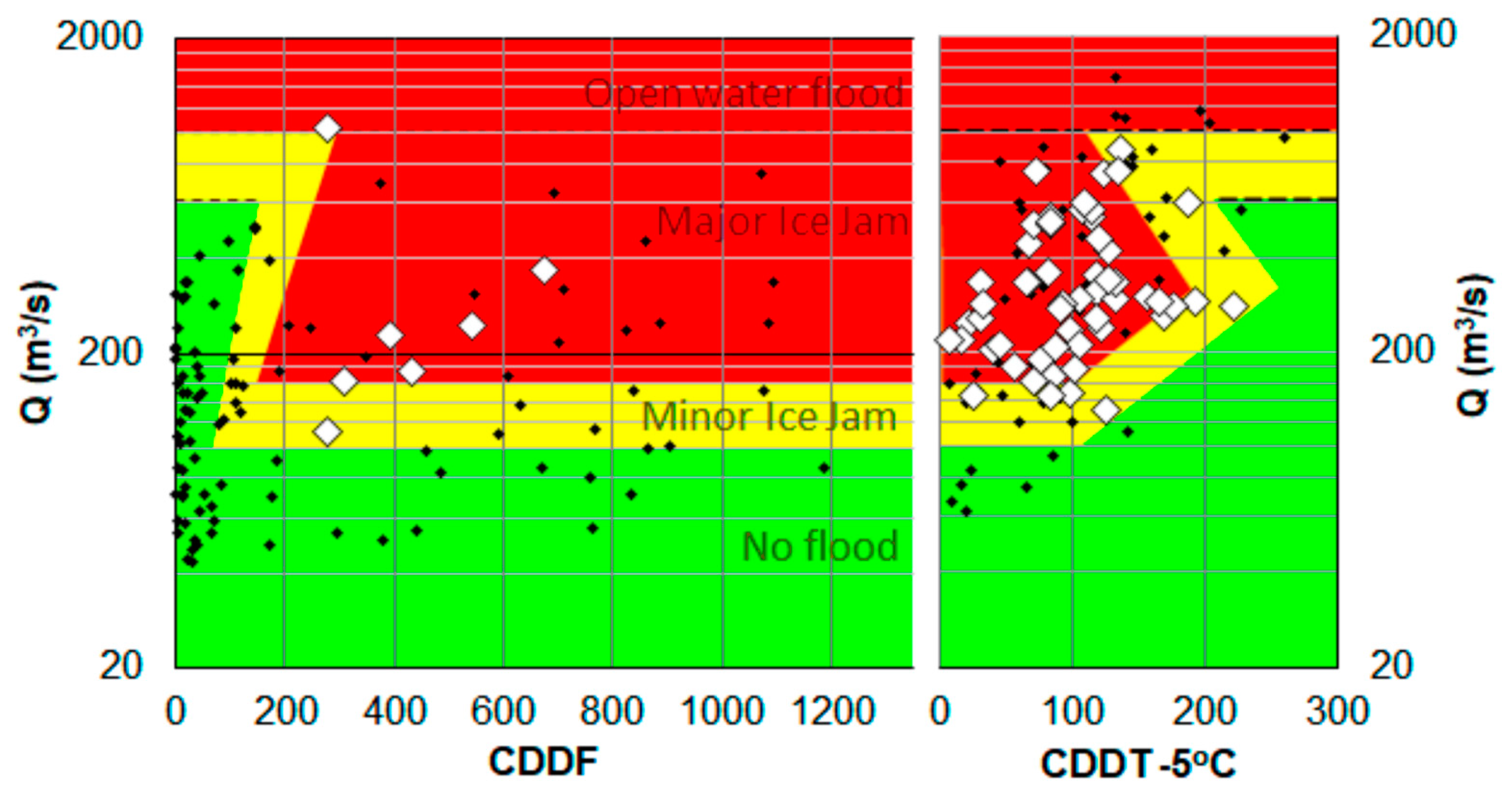
Good hindcasting results for the jam-prone Muskegon River, Michigan, USA, were obtained [22] using peak winter discharge and accumulated degree-days of frost (CDDF) during the cold-weather season. Discharge directly influences the water level attained by an ice jam (Figure 2) and can therefore be regarded as a primary explanatory variable of the flooding potential. The thickness of the winter ice cover can also directly influence ice-jam frequency and severity, but thickness measurements were not available in this study [22], which relied on CDDF as a proxy for pre-melt thickness. Approximate values of the latter were computed using the well-known Stefan equation, which relates thickness to the square root of the CDDF, and an assumed coefficient value [52]. As a rule, the logistic regression was successful: it indicated relatively large probabilities for years with major ice jams and low probabilities for uneventful years.

Logistical regression was also used to study the occurrence of floods caused by ice jams in the lower Peace River, Alberta, one of Canada’s largest rivers [23]. Such events sustain a multitude of high–elevation lakes and ponds (perched basins) located in the Peace Sector of the Peace-Athabasca Delta, a major ecosystem of national and international importance [53]. It was suggested in [23] that optimal results are obtained using two proxy variables: the total winter (November to April) precipitation at a specific meteorological station; and the CDDF at a different meteorological station, both stations being located within the Peace River basin. The authors hypothesized that these variables index breakup discharge potential and end-of-winter ice cover thickness and strength. The results were less clear-cut than those of [22] because the probability estimates for each one of the 55 years of the examined record produced a large “overlap” range (p ~0.2 to 0.7), containing both flood and non-flood years.

8. Climate-Change Projections of IJF Frequency and Severity

Once calibrated, the various methods discussed in previous sessions are, in principle, well suited for studying IJF frequency under a future climate using the results of GCMs and RCMs. As most methods rely on discharge, an obvious approach is to use a hydrological model driven by climate-model output to construct future discharge regimes during key periods of the year, such as freezeup and breakup.

To date, few attempts have been made to assess future IJF frequencies, and even fewer involve the use of hydrological models [48,51,54,55]. The results are not, so far, definitive. For instance, projections made using the model MESH, short for “Modélisation Environnementale communautaire-Surface Hydrology” at sub-daily time steps [21,55], suggest that spring breakup discharges in the Athabasca River at Fort McMurray (Alberta, Canada) will decrease considerably in the future. On the other hand, [54] projects the opposite for the same location using the Variable Infiltration Capacity (VIC) hydrologic model at a monthly time step. More recently, a reanalysis of the MESH model results indicated that peak breakup stages may decrease or increase in the future, depending on how model bias is accounted for [48]. Daily discharge output from the model HYDROTEL (used by the Quebec Government to forecast discharges for several hydrometric stations in this Canadian province) along seven Quebec rivers did not adequately simulate winter and spring discharges in 5 of the 7 rivers [51]. Consequently, it was suggested that the performance of a hydrological model represents the most critical step for climate-change assessment of IJF risk [51]. A similar observation was made in [55].

For ice-jam flooding applications, it is important to know both the magnitude and the timing of breakup (or freezeup) discharges. On the other hand, hydrological models often capture discharge magnitude, but not its timing, or they capture the timing but not the discharge magnitude. Figure 8 shows that the highly sophisticated MESH model does a fair job on spring discharge magnitude but not on timing, even after meticulous calibration [55]. Often, the simulated spring discharges arrive a month or so later than the observed discharges. A real ice jam, occurring in, say, late April due to increasing spring discharge that breaks up the winter ice cover, may cause a major flood (e.g., Fort McMurray, Alberta, Canada, 2020). If the simulated future discharge does not rise until late May, we would project that the winter ice cover would largely decay in place and disintegrate via increasing heat inputs (“thermal” breakup).

The graphical method, which was developed to study seven rivers in Quebec [41], requires very good historical information on the dates of occurrence and on the severity of past ice-jam events, in addition to discharge data. Once “calibrated”, this method can be applied to explore future occurrences under different climate scenarios using future discharges supplied by hydrological modelling. The latter proved largely ineffective in the Quebec rivers study; consequently, Ref. [51] found it necessary to apply considerable judgment in making projections of future ice-jam frequency and severity. Such judgment was founded on “intimate knowledge of each river” as well as on “profound understanding of river ice processes”. It produced concrete projections of future flood risk, which may decrease or increase, depending on river and projected climate scenario.

The difficulties, and labour, associated with hydrological models and their coupling with climate models for IJF projections can be avoided if reliable weather-related proxies for discharge and other relevant controlling variables can be identified. For the ecologically sustaining IJFs of the lower Peace River, the results of the logistic regression, in which discharge potential was indexed by the total winter precipitation (Section 7), were applied to the output of six GCMs and two emission scenarios [23]. The authors projected order-of-magnitude reductions in IJF frequency, depending on model and scenario, but stressed the large uncertainty inherent in such quantifications. Possible causes of such uncertainly are explored in the next section. A large, though less extreme, reduction in IJF frequency for the lower Peace River was also projected [56] via a simpler analysis based on an empirically derived threshold for the Snow Water Equivalent from November to March.

9. Discussion

The hydrotechnical approach is, in principle, the most rigorous for making future projections of the probability distributions of ice-influenced water levels. Physics shows that such distributions depend strongly on the corresponding distributions of the applicable discharges. Under a changed climate, discharges can be assessed using hydrological models, driven by the output of climate models. So far, however, the performance of hydrological models for this purpose has been less than satisfactory, owing to inherent difficulties in correctly simulating both the magnitude and the timing of discharge during key segments of the ice season, such as freezeup and breakup. A common weakness of hydrological models is that they do not adequately account for the presence of ice in a river and for the changing ice conditions during the ice season. It was judiciously recommended in [57] that “Efforts should be concentrated on developing a comprehensive river ice (CRI) model that can simultaneously simulate entire river ice and hydrological processes from freezeup to breakup…” and suggested that this ambitious task will require collaboration among different research groups. This rigorous approach is highly desirable for the long term. An immediate practical, albeit not quite rigorous, “remedy” could be to perform targeted model calibrations, i.e., ascertaining good model performance during a key period of the year, such as breakup, even if this were to result in mediocre performance during other parts of the year.

All hydrotechnical methods require some historical data on peak ice-influenced water levels to calibrate such parameters as the probability of ice-jam occurrence, P(J), for the G-C method, the coefficient k for the Distributed Function Method, or the probability distribution of inflowing ice volume for the MOCAF method. In deciding which method to use in practice, the primary criterion should be performance: does a method adequately reproduce the known stage-frequency distribution? If two or more methods fulfill this requirement equally well, the simplest one would be the optimal choice for making climate-related projections to future SFDs.

Proxy-based methods are less rigorous than the hydrotechnical approach but more convenient because they bypass the hydrological-modelling step. To date, such methods have been applied to binary outcomes (flood, no flood; jam, no jam), though they can conceivably be also applied to non-binary water levels. A good understanding of the strengths and limitations of local candidate proxies is essential to this approach.

For instance, data from the Peace River study [23] indicate that total winter precipitation (snow plus rain, Nov–Apr) at a single station does correlate positively with breakup discharge, but the correlation entails considerable scatter (Figure 9). The non-flood years 2015 and 2020 are just two examples of dissonance between total precipitation and discharge. In 2015, significant thaw and rainfall in March greatly diminished the up-to-then sizeable snowpack so that breakup discharges in April were subdued and well below the least discharge associated with flood years. Interestingly, this rainfall, which was partly responsible for the low breakup discharge, augmented the Nov–Apr precipitation. In 2020, the precipitation proxy was about the same as its average value over the examined time period, resulting in a near-zero flood probability. On the other hand, 2020 breakup discharges were extreme, matching those of the 1974 breakup and jamming, which inundated most of the delta over a period of 10 to 14 days [58].

The accumulated degree-days of frost is another commonly used proxy, widely postulated to index the end-of-winter or maximum thickness of the ice cover. Experience indicates that ice thickness does correlate positively with CDDF, but such correlations can come with considerable scatter [59]. This is likely due to the fact that factors other than air temperature also influence ice growth, such as intensity and temporal distribution of snowfall, as well as frequency and duration of snow-ice formation episodes. A seminal paper on ice thickening and thinning [60] concluded that “…the largest variations from year to year at a given site are associated with the thickness of the snow on the ice, and secondarily by variations in the coldness of the winter period of thickening”.

An additional source of uncertainty in using statistical regression for projecting future IJF frequency arises from the assumption of a linear relationship between the dependent variable (e.g., the logit in logistic regression or the water level in simple regression) and the selected explanatory independent variables. There is no guarantee that such a relationship is valid, and most likely it is not, since a linear function is one of infinitely many nonlinear functions that could involve products, as well as powers, exponents, or logarithms of the explanatory variables. Without any physical justification for the assumed linearity, the extrapolation of a regression equation to significantly different climatic conditions may or may not furnish credible results.

10. Limitations and Research Needs

As already outlined in the preceding sections, all reviewed methods are subject to limitations. Starting with the G-C method, there is no guarantee that the occurrence probability of an ice jam, P(J), is independent of discharge. A trial calculation for a specific river site indicated that P(J) should decrease with discharge to achieve a good match between calculated and observed SFDs [20]. Additional tests of the G-C method are needed to learn more about how P(J) might be related to discharge. The same applies to the DFM, which relies on the empirical coefficient k. So far, k is known to range from 0.6 to 0.9, based on data from 4 river sites. Testing this method on numerous additional sites would better define the range of k and potentially reveal a relationship between k and local channel morphology.

In all discharge-based stage-frequency analysis methods, the correct discharge value applies to the time when the peak stage occurs. In practical applications, this time will not be known unless the site of interest is a hydrometric gauge with very good historical records of the water level. In such instances, the maximum discharge value that occurred during each breakup (or freezeup) event should be used to ensure that any associated errors will be on the conservative side. Conservative errors will also occur if there are upper limits to the peak water level and/or to the associated breakup discharge. Such limits can only be determined by careful examination of local conditions, and especially of the configuration of the floodplain.

A key element of the MOCAF approach is the volume of ice rubble contained in an ice jam. Though it has been assumed to vary randomly and independently of discharge, physical considerations suggest that this volume should increase with discharge, though such a relationship would likely involve scatter. Research on this issue would involve a combination of annual field observations to determine ice jam extent and severity, plus modelling to match observed water levels and thence infer the applicable ice volume. Data over a multi-year period could help define the ice volume-discharge relationship.

Rigorous assessment of future peak stages caused by ice jams under different climatic scenarios requires a hydrological model to “translate” arrays of seasonal climatic variables to breakup (or freezeup) discharges. The few such applications to date revealed weaknesses in the predictive capacity of hydrological models when applied to the winter/spring periods. As suggested in [57], overcoming this difficulty will require a concerted, long-term research effort.

At present, all of the discussed methods involve uncertainty when applied to make projections of IJF risk under future climatic scenarios. As stated in [51], case-by-case studies require application of judgment based on intimate knowledge of each river and its ice processes. Such knowledge can be enhanced by systematic annual observations of ice formation, evolution, and breakup.

11. Summary and Conclusions

Several methods have been proposed for constructing stage-frequency distributions of ice-influenced annual peaks in cases in which historical stage data are scarce or completely unavailable. These methods largely belong to the hydrotechnical approach, which relies on historical discharge data during the ice season and ranges in complexity from the simple discrete-outcomes method to the complex and computationally demanding Monte Carlo Framework. If no stage data are available for calibration, hydrotechnical methods can help explore scenarios generated by assuming plausible coefficients or ice volumes based on local experience regarding ice-jam susceptibility or on past experience in rivers of similar magnitude, hydrograph, and ice thickness. Application of hydrotechnical methods to future climate scenarios requires prediction of future discharges, which can be accomplished using hydrological models driven by the output of selected climate models. Though this is the most rigorous approach, the predictive capability of hydrological models appears at present to be limited for the intended purpose, which requires good simulation of both the magnitude and the timing of discharge during the breakup (or freezeup) period. Possible approaches to deal with this difficulty include developing hydrological models that integrate river ice processes in the long term, or targeting calibration of existing models to specific parts of the year in the short term. Proxy-based methods can be applied directly to climate-model output to assess IJF probability using logistic regression; uncertainty arises from occasional dissonance between proxy and primary explanatory variables, and from nonlinear dependency of the logit on such variables.