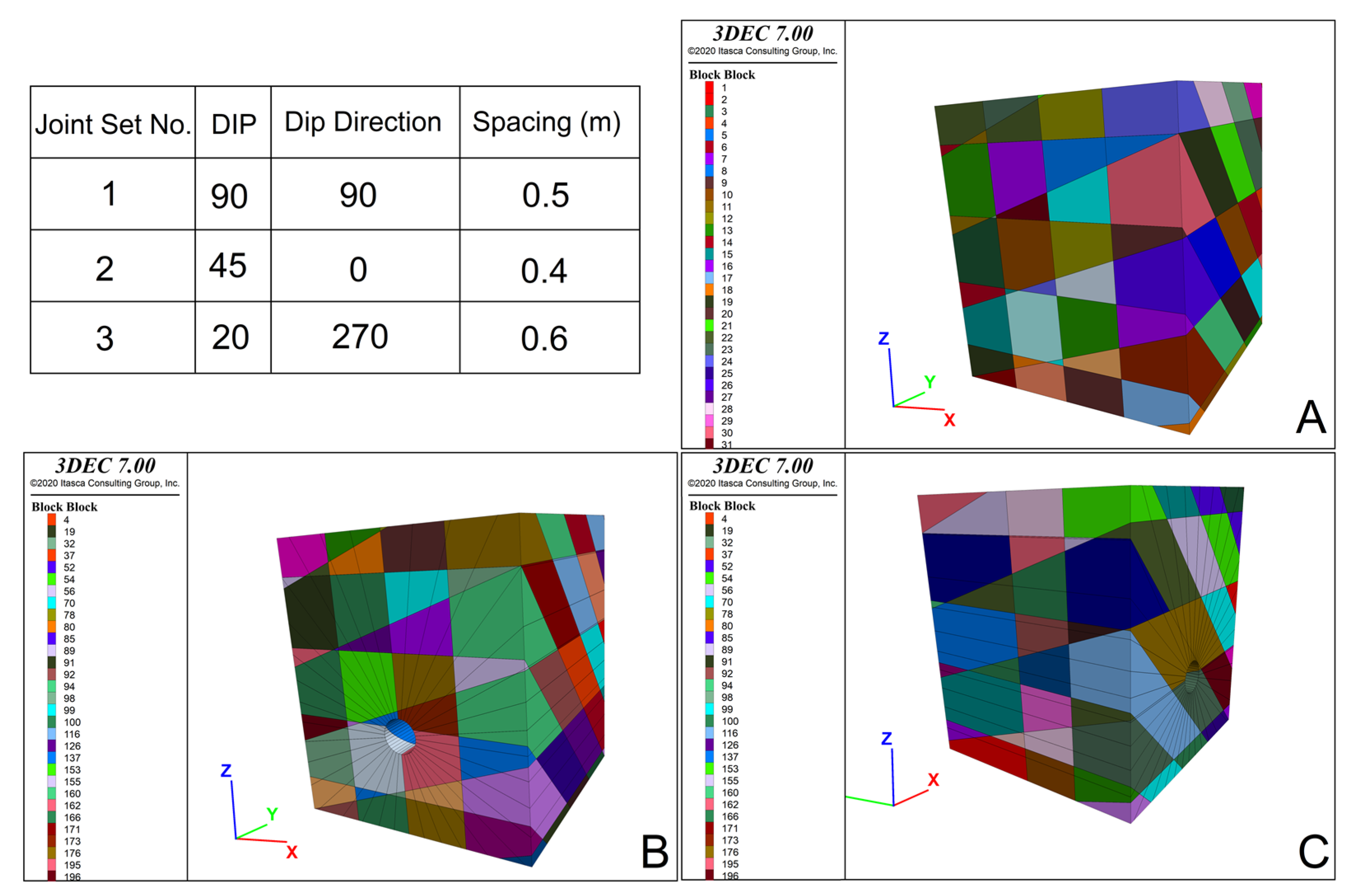
Figure 1.
Modes of excavation of the tunnel in a fractured rock mass, (A) predetermined REV of the rock mass, (B) excavation of a horizontal tunnel in the y-direction of model A, and (C) excavation of the horizontal tunnel in the x-direction.
Figure 1.
Modes of excavation of the tunnel in a fractured rock mass, (A) predetermined REV of the rock mass, (B) excavation of a horizontal tunnel in the y-direction of model A, and (C) excavation of the horizontal tunnel in the x-direction.
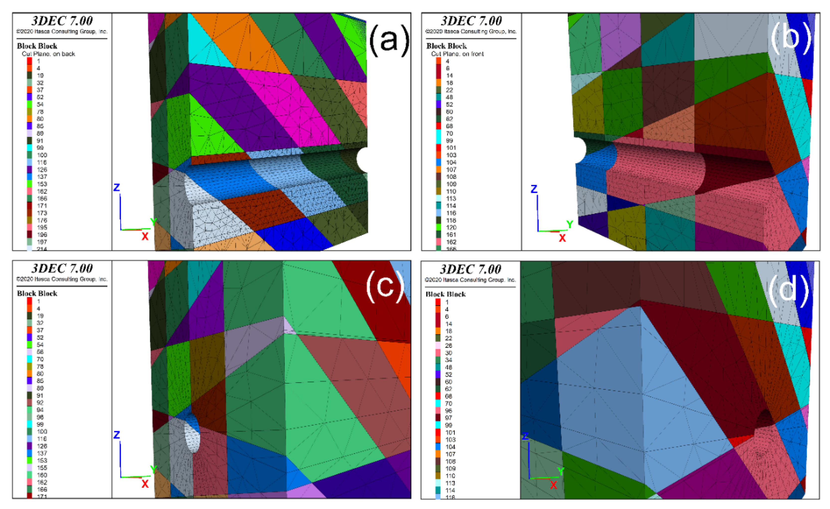
Figure 2.
Longitudinal cross-section of the tunnel that is excavated in (a) x-direction, (b) y-direction, (c) and (d) original tunnel of the case (a) and (b), respectively.
Figure 2.
Longitudinal cross-section of the tunnel that is excavated in (a) x-direction, (b) y-direction, (c) and (d) original tunnel of the case (a) and (b), respectively.
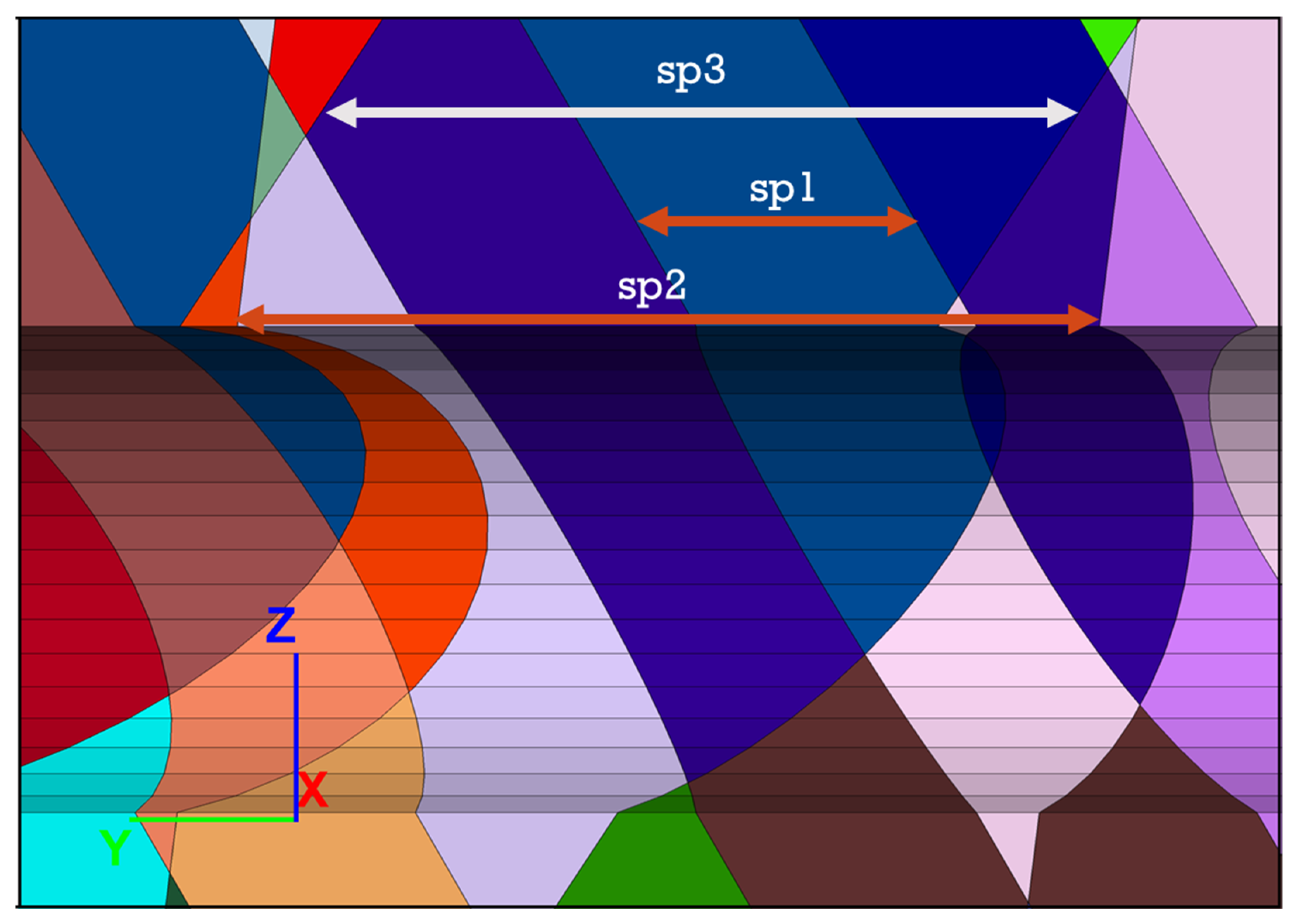
Figure 3.
Apparent spacings of each joint set at the wall of the tunnel: sp1, sp2, and sp3 are the apparent spacings of the joint set 1, joint set 2, and joint set 3, respectively.
Figure 3.
Apparent spacings of each joint set at the wall of the tunnel: sp1, sp2, and sp3 are the apparent spacings of the joint set 1, joint set 2, and joint set 3, respectively.
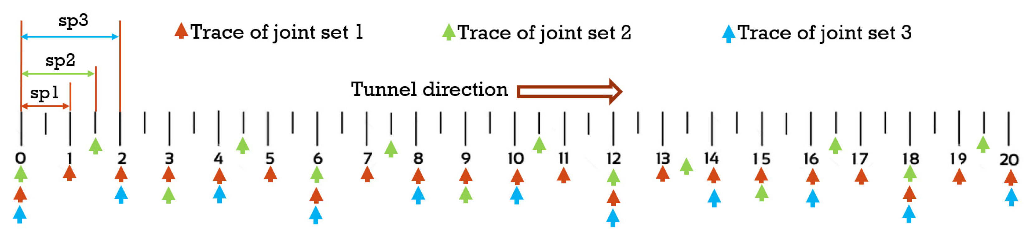
Figure 4.
Locations of the traces of joint sets at the wall of the tunnel excavated in a rock mass and includes three joint sets: sp1, sp2, and sp3 are the apparent spacings of joint set 1, joint set 2, and joint set 3, respectively.
Figure 4.
Locations of the traces of joint sets at the wall of the tunnel excavated in a rock mass and includes three joint sets: sp1, sp2, and sp3 are the apparent spacings of joint set 1, joint set 2, and joint set 3, respectively.
Figure 5.
A rock mass including three joint sets with apparent spacings equal to 0.1, 1, and 6 m, (a) cross-section of the tunnel along its direction showing the repeating pattern of the discontinuities in the direction of the tunnel and 3rd set’s apparent spacing (6 m), (b) apparent spacings of 1st and 2nd joint sets, (c) close up of the section of the tunnel that includes STL, and (d) and (e) close up of the beginning and end of the STL showing the existence of an analogous pattern at both ends.
Figure 6.
Specifying the apparent spacing of a joint set at the wall of the tunnel; (a) Ɵi is the angle between normal to joint set and direction of the tunnel, and (b) variation of the joint spacing by deviation from the perpendicular cross of the tunnel and fracture plane.
Figure 6.
Specifying the apparent spacing of a joint set at the wall of the tunnel; (a) Ɵi is the angle between normal to joint set and direction of the tunnel, and (b) variation of the joint spacing by deviation from the perpendicular cross of the tunnel and fracture plane.
Figure 7.
Numerical models for validation of the existence of the STL using 3DEC software; the tunnel in all cases is excavated in the y-direction (S-N).
Figure 7.
Numerical models for validation of the existence of the STL using 3DEC software; the tunnel in all cases is excavated in the y-direction (S-N).
Figure 8.
Boundary conditions and calculation methods applied in numerical simulations; (a) flow planes or the planes of the fractures, (b) pore pressure around the tunnel in a flow plane, and (c) flow plane zones selected for calculation of the inflow rate to the tunnel.
Figure 8.
Boundary conditions and calculation methods applied in numerical simulations; (a) flow planes or the planes of the fractures, (b) pore pressure around the tunnel in a flow plane, and (c) flow plane zones selected for calculation of the inflow rate to the tunnel.
Figure 9.
Average inflow rate to the tunnel for half STL (0.5 STL), 1 STL, 1.5 STL, 2 STL, and 3 STL: the diagram shows that the average inflow rate is equal for the tunnels with 1 STL, 2 STL, and 3 STL but differs for the 0.5 STL and 1.5 STL.
Figure 9.
Average inflow rate to the tunnel for half STL (0.5 STL), 1 STL, 1.5 STL, 2 STL, and 3 STL: the diagram shows that the average inflow rate is equal for the tunnels with 1 STL, 2 STL, and 3 STL but differs for the 0.5 STL and 1.5 STL.
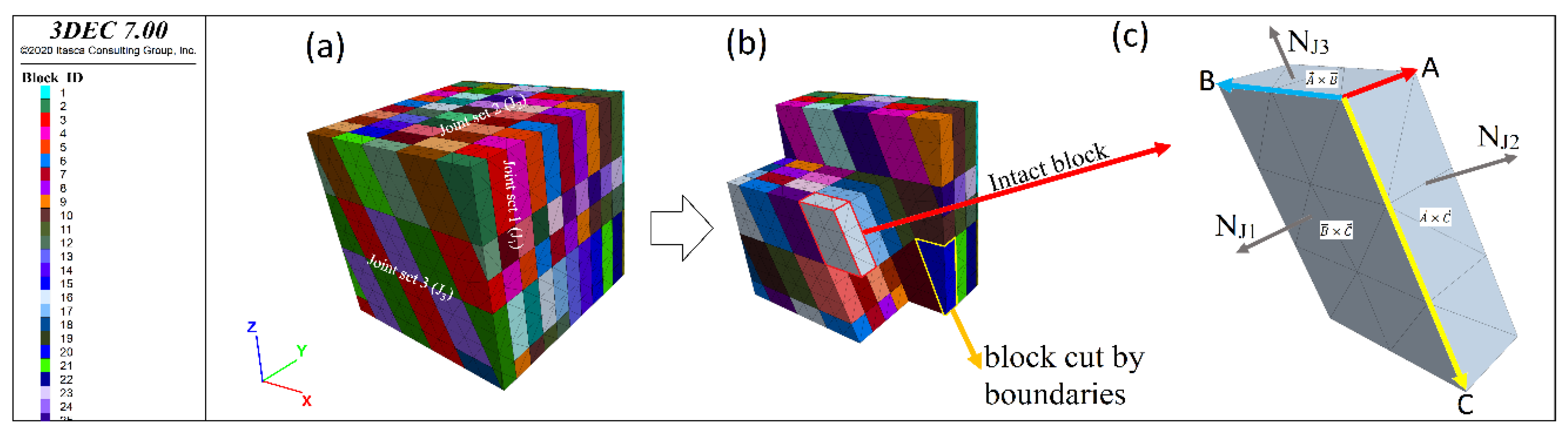
Figure 10.
Methodology used for analytical calculation of the block surface area: (a) a model comprising of three joint sets, (b) selected block not cut by the boundaries of the model, and (c) edge vectors and surface area of each side of the selected block.
Figure 10.
Methodology used for analytical calculation of the block surface area: (a) a model comprising of three joint sets, (b) selected block not cut by the boundaries of the model, and (c) edge vectors and surface area of each side of the selected block.
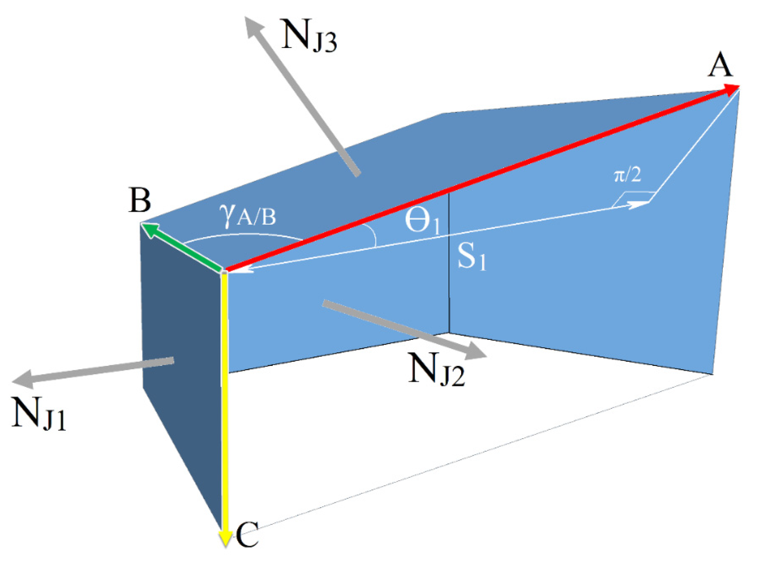
Figure 11.
Inner view of an intact block. Edge vectors of the block and the angles between the true spacing of joint set 1 and direction of the edge vector A (Ɵ1). Ɵ2 and Ɵ3 could be specified with the same method. γA/B, γA/C, and γB/C are the angles between edge vectors A&B, A&C, and B&C, respectively.
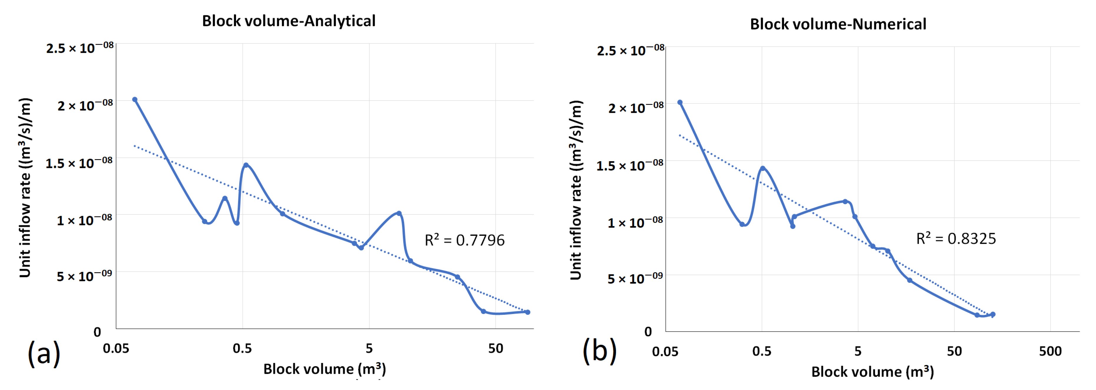
Figure 12.
Relationship between inflow rate to the tunnel and logarithm of RBLV that is calculated using (a) analytical and (b) numerical methods.
Figure 12.
Relationship between inflow rate to the tunnel and logarithm of RBLV that is calculated using (a) analytical and (b) numerical methods.
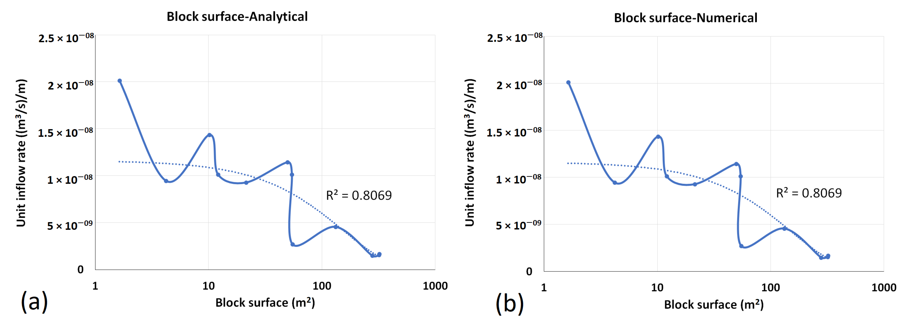
Figure 13.
Relationship between the inflow rate and logarithm of RBLS calculated using (a) analytical and (b) numerical methods.
Figure 13.
Relationship between the inflow rate and logarithm of RBLS calculated using (a) analytical and (b) numerical methods.
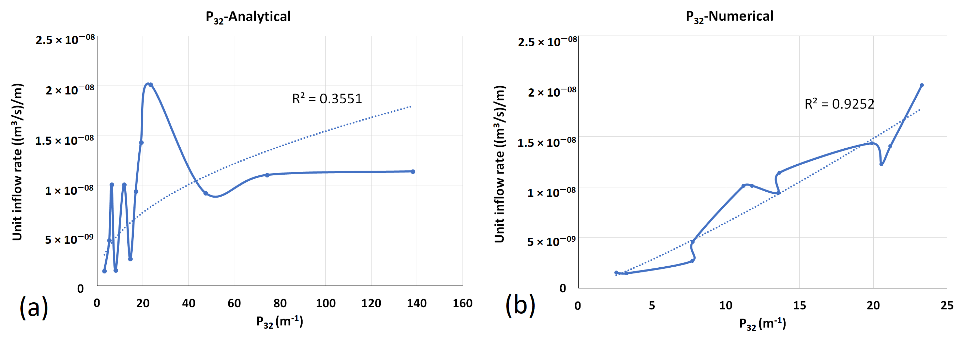
Figure 14.
Relationship between the inflow rate and the 3D fracture intensity (P32) that is calculated (a) analytically and (b) numerically.
Figure 14.
Relationship between the inflow rate and the 3D fracture intensity (P32) that is calculated (a) analytically and (b) numerically.
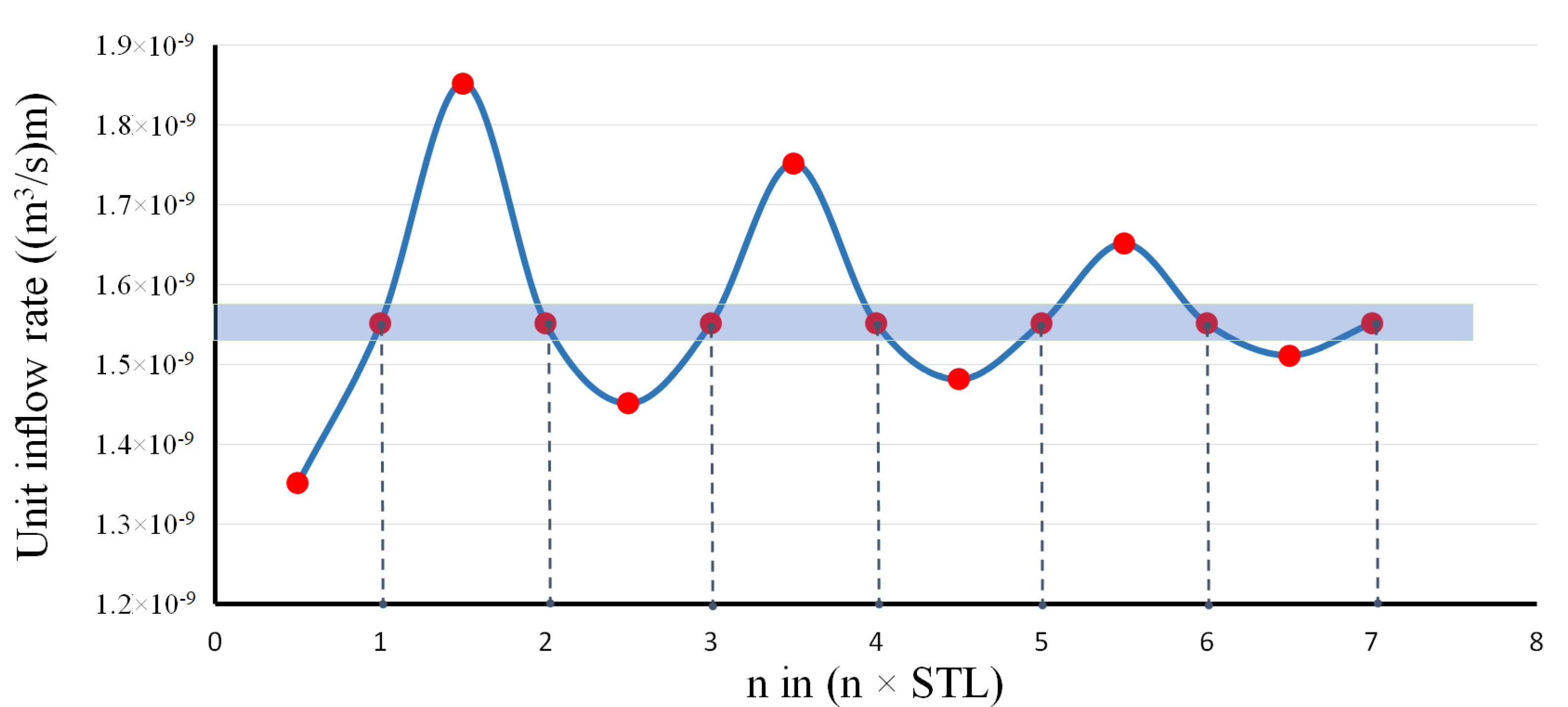
Figure 15.
Variations of the inflow rate with the tunnel length as the multiple of STL for case number 10 of
Table 3. The inflow rate to the tunnel with a length equal to 1STL is the same as that for the length of tunnel equal to n × STL.
Figure 15.
Variations of the inflow rate with the tunnel length as the multiple of STL for case number 10 of
Table 3. The inflow rate to the tunnel with a length equal to 1STL is the same as that for the length of tunnel equal to n × STL.
Table 1.
Joint set characteristics considered in the numerical models for assessment of the STL (DIP, DD, S, and Ap are the dip, dip direction, true spacings, and hydraulic aperture of the joint sets, respectively).
Table 1.
Joint set characteristics considered in the numerical models for assessment of the STL (DIP, DD, S, and Ap are the dip, dip direction, true spacings, and hydraulic aperture of the joint sets, respectively).
| | Joint Set 1 | Joint Set 2 | Joint Set 3 | Tunnel Diameter (m) | Water Head (m) |
|---|
| Case No. | DIP | DD | S (cm) | Ap (cm) | DIP | DD | S (cm) | Ap (cm) | DIP | DD | S (cm) | Ap (cm) |
|---|
| 1 | 22 | 25 | 205.2 | 1 × 10⁻⁴ | 21 | 342 | 205.2 | 1 × 10⁻⁴ | 80 | 0 | 9.8 | 1 × 10⁻⁴ | 1 | 5 |
| 2 | 81 | 5 | 39.4 | 1 × 10⁻⁴ | 73 | 25 | 519.6 | 1 × 10⁻⁴ | 82 | 354 | 98.5 | 1 × 10⁻⁴ |
| 3 | 86 | 9 | 590.9 | 1 × 10⁻⁴ | 67 | 340 | 8.7 | 1 × 10⁻⁴ | 80 | 0 | 590.9 | 1 × 10⁻⁴ |
| 4 | 84 | 8 | 590.9 | 1 × 10⁻⁴ | 86 | 351 | 590.9 | 1 × 10⁻⁴ | 80 | 0 | 590.9 | 1 × 10⁻⁴ |
| 5 | 61 | 8 | 8.7 | 1 × 10⁻⁴ | 21 | 342 | 13.7 | 1 × 10⁻⁴ | 80 | 2 | 9.8 | 1 × 10⁻⁴ |
Table 2.
The apparent spacings (Sp1, Sp2, and Sp3) at the wall of the tunnel for each model, STL, and the value of the inflow rate to the tunnel for the tunnel length of 0.5 STL, 1 STL, 1.5 STL, 2 STL, and 3 STL.
Table 2.
The apparent spacings (Sp1, Sp2, and Sp3) at the wall of the tunnel for each model, STL, and the value of the inflow rate to the tunnel for the tunnel length of 0.5 STL, 1 STL, 1.5 STL, 2 STL, and 3 STL.
| | | | | | Inflow Rate (m3/s) per Meter of Tunnel Length |
|---|
| Case No. | Sp1 (m) | Sp2 (m) | Sp3 (m) | STL (m) | 0.5 STL | 1.0 STL | 1.5 STL | 2.0 STL | 3.0 STL |
|---|
| 1 | 6 | 6 | 0.1 | 6 | 2.15 × 10⁻⁸ | 9.35 × 10⁻¹⁰ | 1.02 × 10⁻⁸ | 9.35 × 10⁻¹⁰ | 9.35 × 10⁻¹⁰ |
| 2 | 0.4 | 6 | 1 | 6 | 7.15 × 10⁻¹⁰ | 3.58 × 10⁻¹⁰ | 9.41 × 10⁻¹⁰ | 3.58 × 10⁻¹⁰ | 3.58 × 10⁻¹⁰ |
| 3 | 6 | 0.1 | 6 | 6 | 1.28 × 10⁻⁸ | 1.51 × 10⁻⁸ | 1.36 × 10⁻⁸ | 1.51 × 10⁻⁸ | 1.52 × 10⁻⁸ |
| 4 | 6 | 6 | 6 | 6 | 5.96 × 10⁻¹⁰ | 8.98 × 10⁻¹⁰ | 1.50 × 10⁻⁹ | 8.98 × 10⁻¹⁰ | 8.98 × 10⁻¹⁰ |
| 5 | 0.1 | 0.4 | 0.1 | 0.4 | 7.15 × 10⁻¹⁰ | 8.28 × 10⁻¹⁰ | 5.96 × 10⁻⁹ | 8.28 × 10⁻¹⁰ | 5.96 × 10⁻¹⁰ |
Table 3.
Characteristics of the discontinuities used for comparison of analytical and numerical calculation of the block volume and block surface and also assessing the effects of the block characteristics on the inflow rate to the tunnel.
Table 3.
Characteristics of the discontinuities used for comparison of analytical and numerical calculation of the block volume and block surface and also assessing the effects of the block characteristics on the inflow rate to the tunnel.
| | Joint Set 1 | Joint Set 2 | Joint Set 3 |
|---|
| Case | DIP | DD | Spacing (m) | Ap (m) | DIP | DD | Spacing (m) | Ap (m) | DIP | DD | Spacing (m) | Ap (m) |
|---|
| 1 | 23 | 30 | 0.34 | 2 × 10⁻⁵ | 20 | 10 | 2.05 | 5 × 10⁻⁷ | 27 | 320 | 0.14 | 2 × 10⁻⁵ |
| 2 | 90 | 350 | 0.39 | 2 × 10⁻⁵ | 20 | 352 | 0.14 | 2 × 10⁻⁵ | 90 | 10 | 0.39 | 5 × 10⁻⁶ |
| 3 | 73 | 25 | 0.35 | 5 × 10⁻⁶ | 61 | 352 | 0.35 | 2 × 10⁻⁵ | 84 | 8 | 5.91 | 5 × 10⁻⁶ |
| 4 | 22 | 25 | 0.34 | 5 × 10⁻⁷ | 90 | 350 | 0.98 | 2 × 10⁻⁵ | 60 | 0 | 0.35 | 2 × 10⁻⁵ |
| 5 | 90 | 350 | 0.39 | 5 × 10⁻⁶ | 90 | 10 | 0.39 | 5 × 10⁻⁷ | 32 | 50 | 2.05 | 2 × 10⁻⁵ |
| 6 | 90 | 350 | 5.91 | 5 × 10⁻⁷ | 90 | 70 | 0.14 | 5 × 10⁻⁶ | 90 | 30 | 5.2 | 5 × 10⁻⁶ |
| 7 | 20 | 350 | 0.34 | 2 × 10⁻⁵ | 22 | 25 | 1.37 | 2 × 10⁻⁵ | 61 | 354 | 5.2 | 5 × 10⁻⁶ |
| 8 | 54 | 65 | 0.34 | 2 × 10⁻⁵ | 90 | 350 | 0.98 | 5 × 10⁻⁶ | 90 | 30 | 0.35 | 5 × 10⁻⁶ |
| 9 | 80 | 0 | 5.91 | 5 × 10⁻⁶ | 90 | 70 | 0.14 | 5 × 10⁻⁷ | 66 | 292 | 0.34 | 5 × 10⁻⁶ |
| 10 | 60 | 0 | 3.46 | 2 × 10⁻⁵ | 67 | 340 | 5.2 | 5 × 10⁻⁶ | 90 | 30 | 0.87 | 5 × 10⁻⁶ |
| 11 | 90 | 30 | 3.46 | 5 × 10⁻⁶ | 54 | 295 | 1.37 | 5 × 10⁻⁶ | 80 | 0 | 3.94 | 5 × 10⁻⁷ |
| 12 | 90 | 70 | 0.34 | 2 × 10⁻⁵ | 43 | 300 | 1.37 | 5 × 10⁻⁷ | 73 | 25 | 5.2 | 5 × 10⁻⁷ |
| 13 | 43 | 60 | 0.14 | 5 × 10⁻⁷ | 73 | 335 | 5.2 | 5 × 10⁻⁷ | 90 | 10 | 0.39 | 2 × 10⁻⁵ |
Table 4.
Comparison of the analytical and numerical calculation of the block volume (RBLV) and block surface (RBLS) for the cases of
Table 3. N/A means that the parameter is unmeasurable.
Table 4.
Comparison of the analytical and numerical calculation of the block volume (RBLV) and block surface (RBLS) for the cases of
Table 3. N/A means that the parameter is unmeasurable.
| | Block Surface (RBLS) (m2) | Block Volume (RBLV) (m3) |
|---|
| Case | Analytical (This Study) | Numerical (3DEC) | Analytical [23] | Numerical (3DEC) |
|---|
| 1 | 320.2 | 320.2 | 4.31 | 15.14 |
| 2 | 1.63 | 1.63 | 0.07 | 0.07 |
| 3 | 54.15 | 54.16 | 8.55 | 4.6 |
| 4 | 49.73 | 49.71 | 0.36 | 3.65 |
| 5 | 12.08 | 12.07 | 1.03 | 1.08 |
| 6 | N/A | N/A | 10.57 | N/A |
| 7 | 131.54 | 131.53 | 24.90 | 17.02 |
| 8 | 4.21 | 4.20 | 0.25 | 0.31 |
| 9 | 21.35 | 21.35 | 0.45 | 1.04 |
| 10 | 278.38 | 278.39 | 89.33 | 85.36 |
| 11 | 317.93 | 318.04 | 39.91 | 124.94 |
| 12 | 54.75 | 54.75 | 3.80 | 7.09 |
| 13 | 10.15 | 10.14 | 0.53 | 0.51 |
Table 5.
Geometrical and hydrogeological characteristics of the tunnel and rock mass for evaluation of the impact of rock geometries on inflow rate.
Table 5.
Geometrical and hydrogeological characteristics of the tunnel and rock mass for evaluation of the impact of rock geometries on inflow rate.
| Case No. | 1 | 2 | 3 | 4 | 5 | 6 | 7 | 8 | 9 | 10 | 11 | 12 | 13 |
|---|
| Water head (m) | 40 | 10 | 10 | 10 | 40 | 100 | 10 | 40 | 40 | 40 | 40 | 100 | 10 |
| Tunnel radius (m) | 4 | 1 | 4 | 4 | 2 | 4 | 1 | 2 | 4 | 1 | 1 | 4 | 1 |


