
An Open-Source Code for Fluid Flow Simulations in Unconventional Fractured Reservoirs


Abstract
1. Introduction
2. Physicomathematical Statements
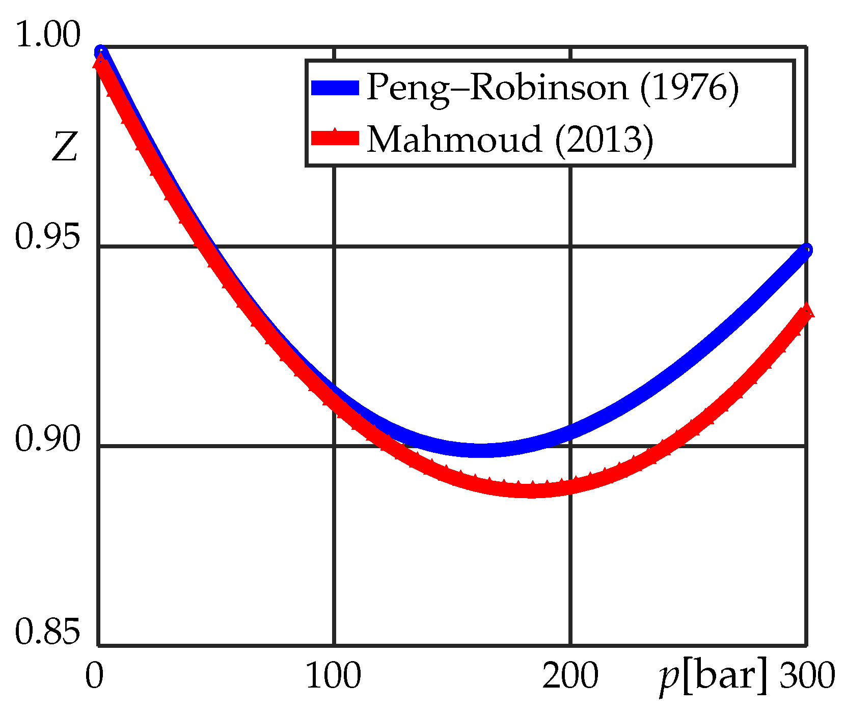
2.1. Gas Density
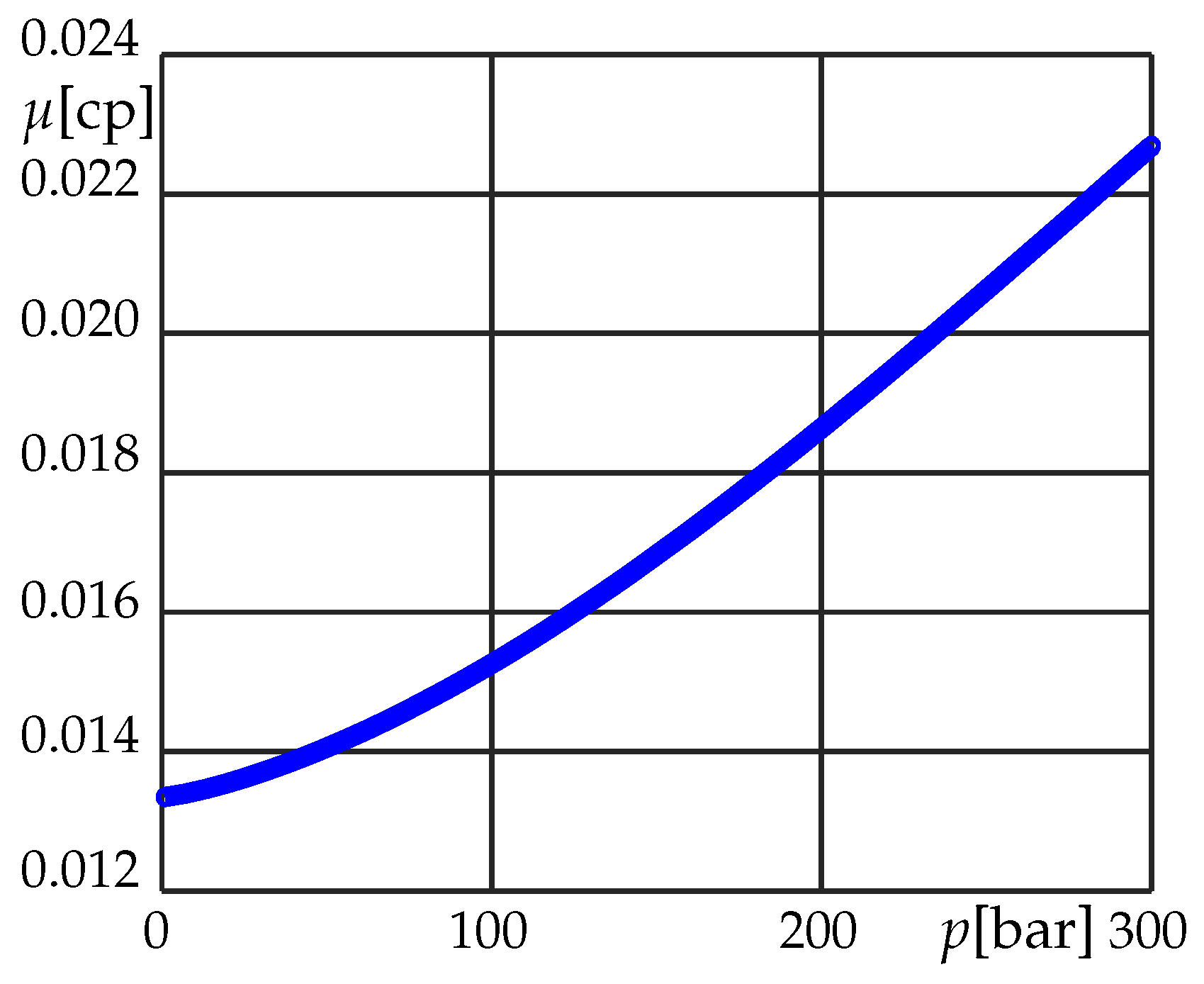
2.2. Gas Viscosity
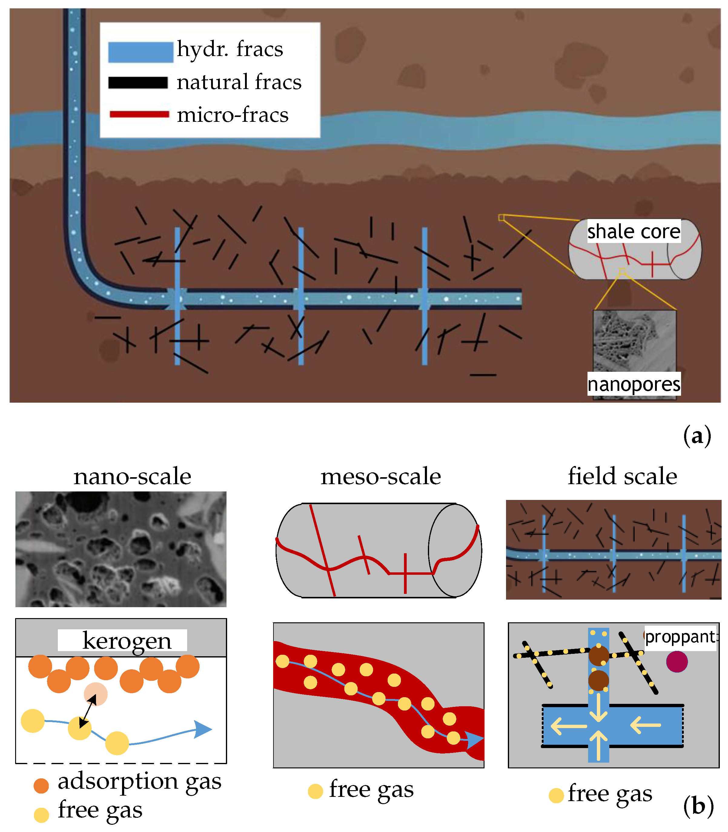
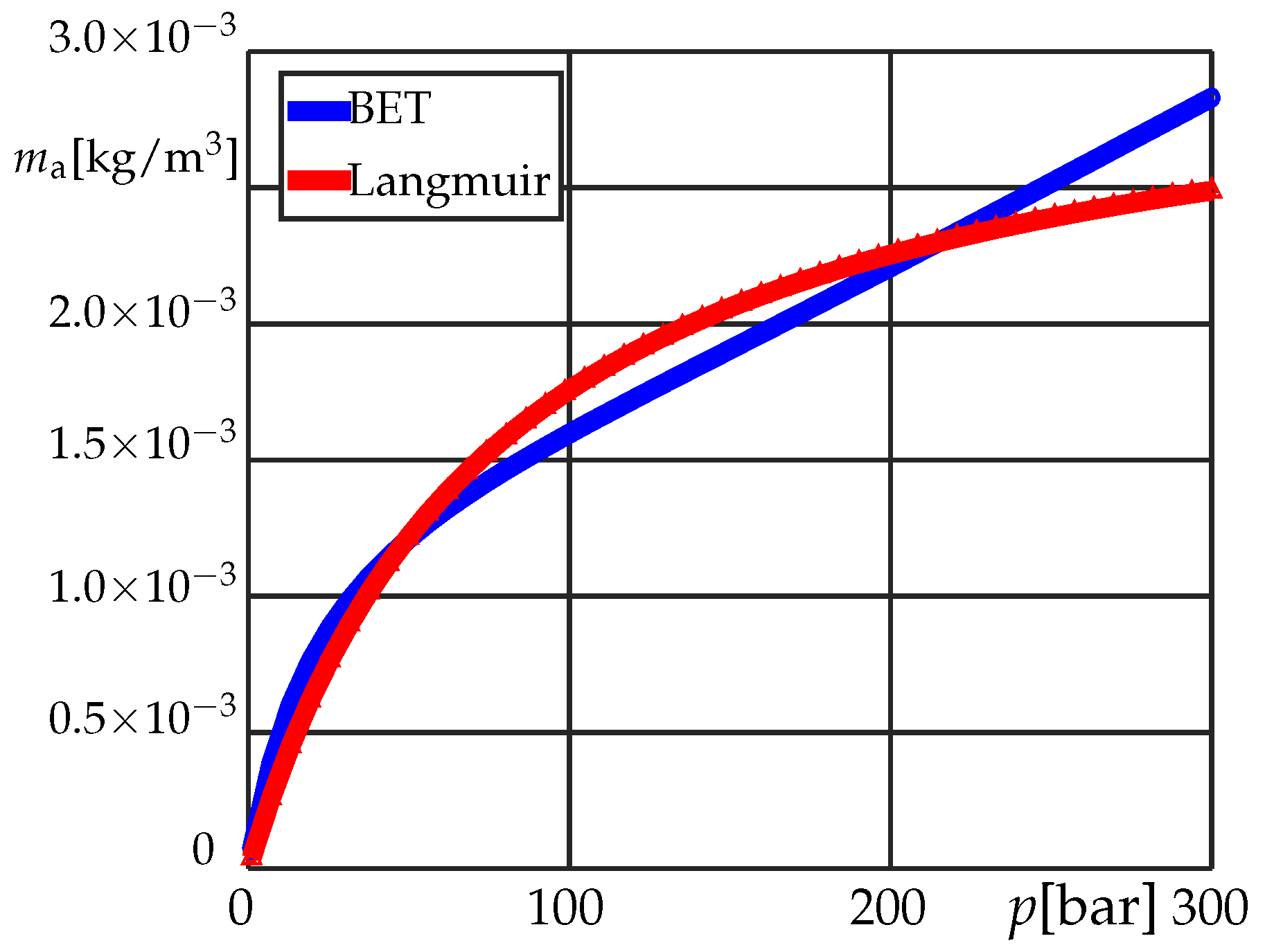
2.3. Adsorption and Transport
2.4. Indirect Hydromechanical Coupling
3. The Numerical Model
3.1. Numerical Discretization
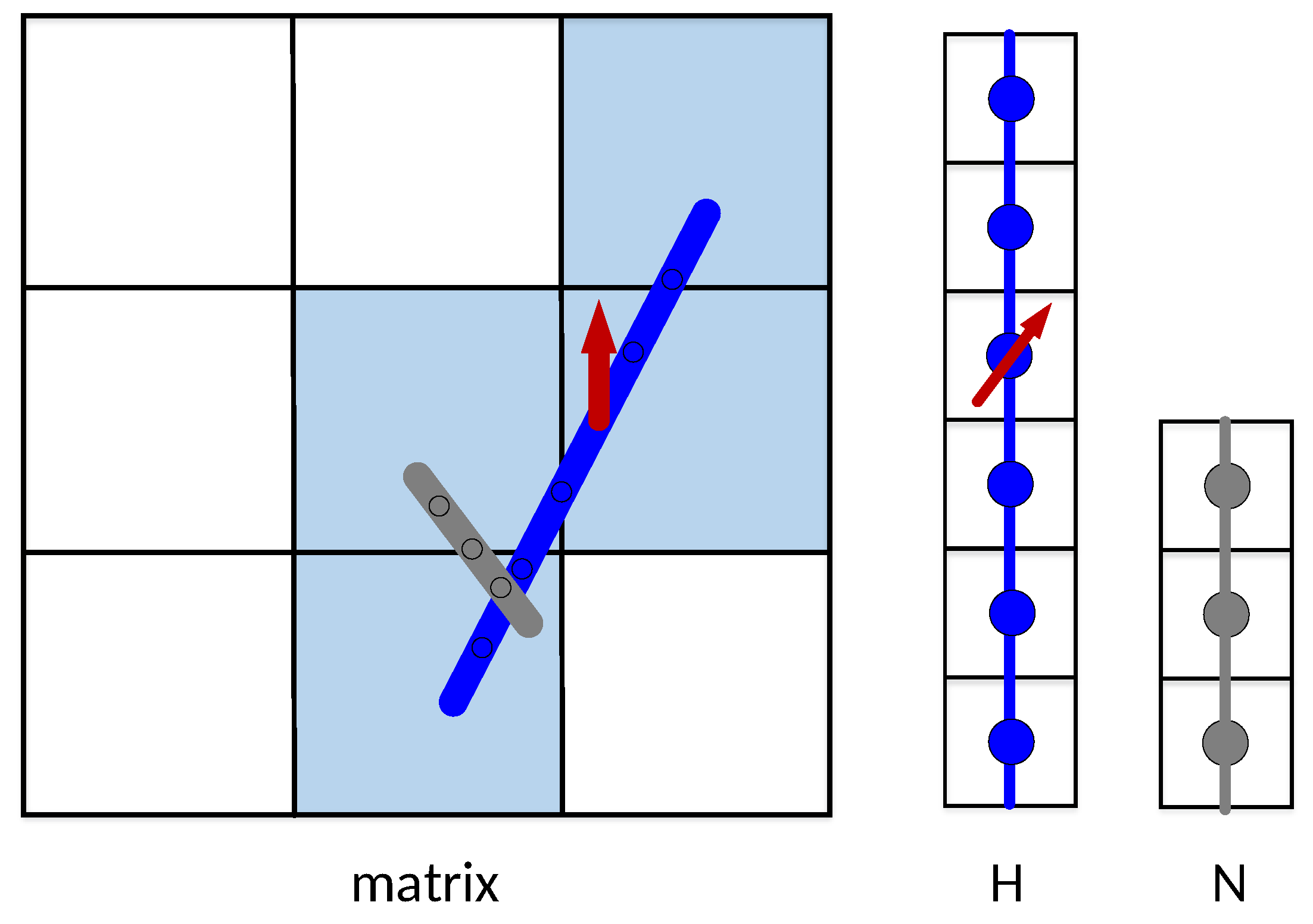
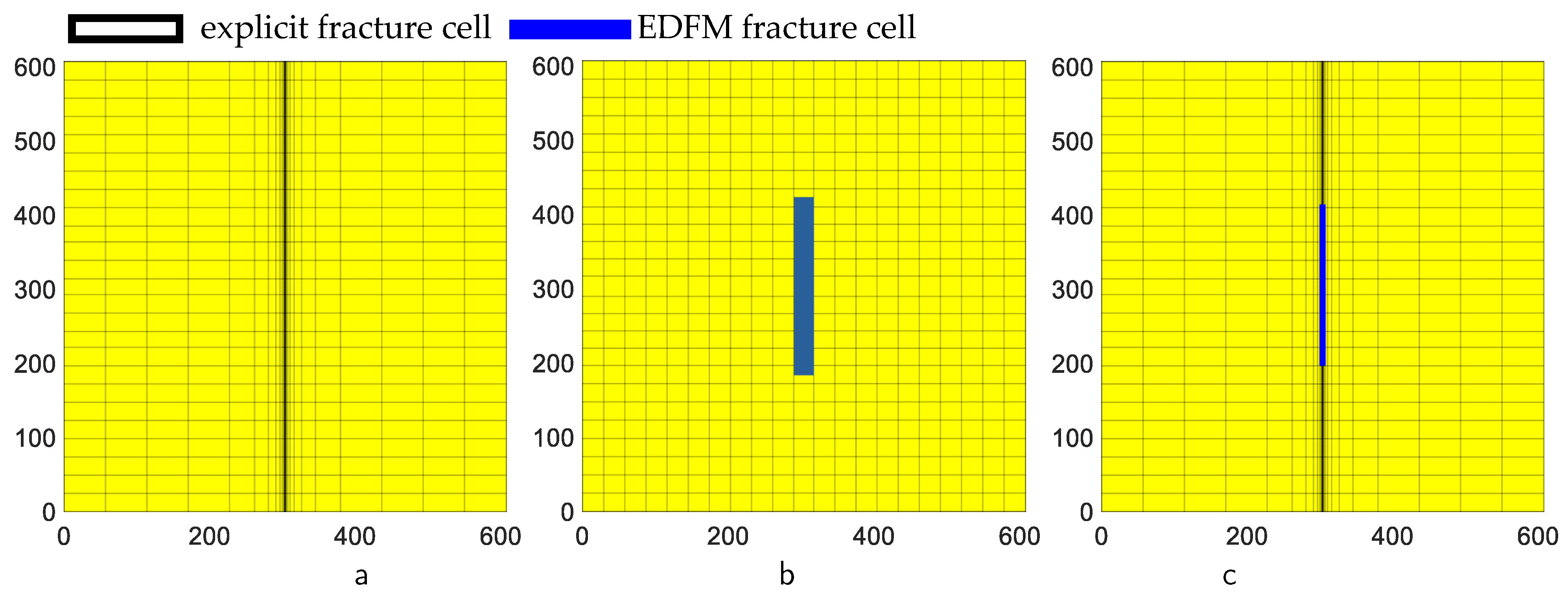
3.2. EDFM
4. Validation
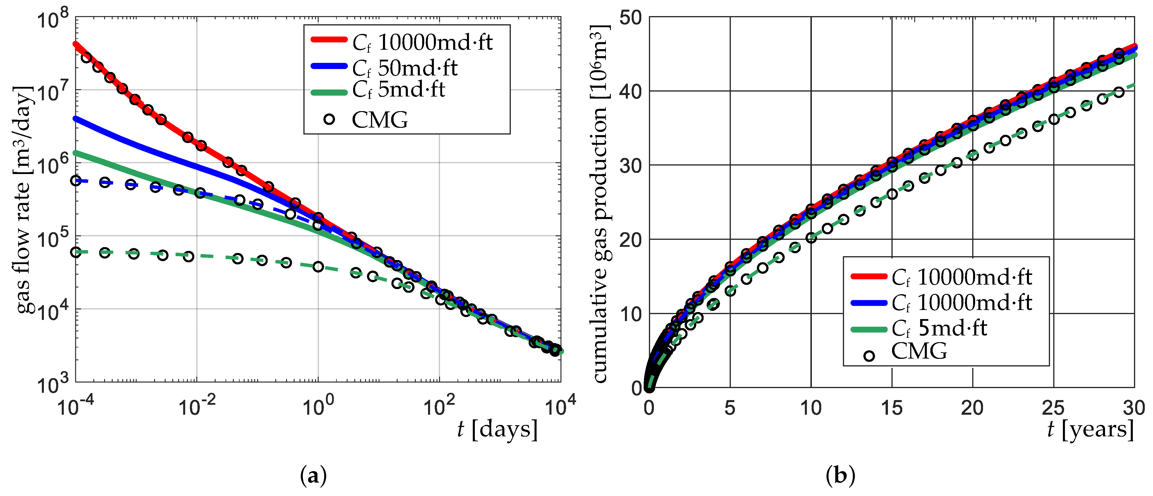
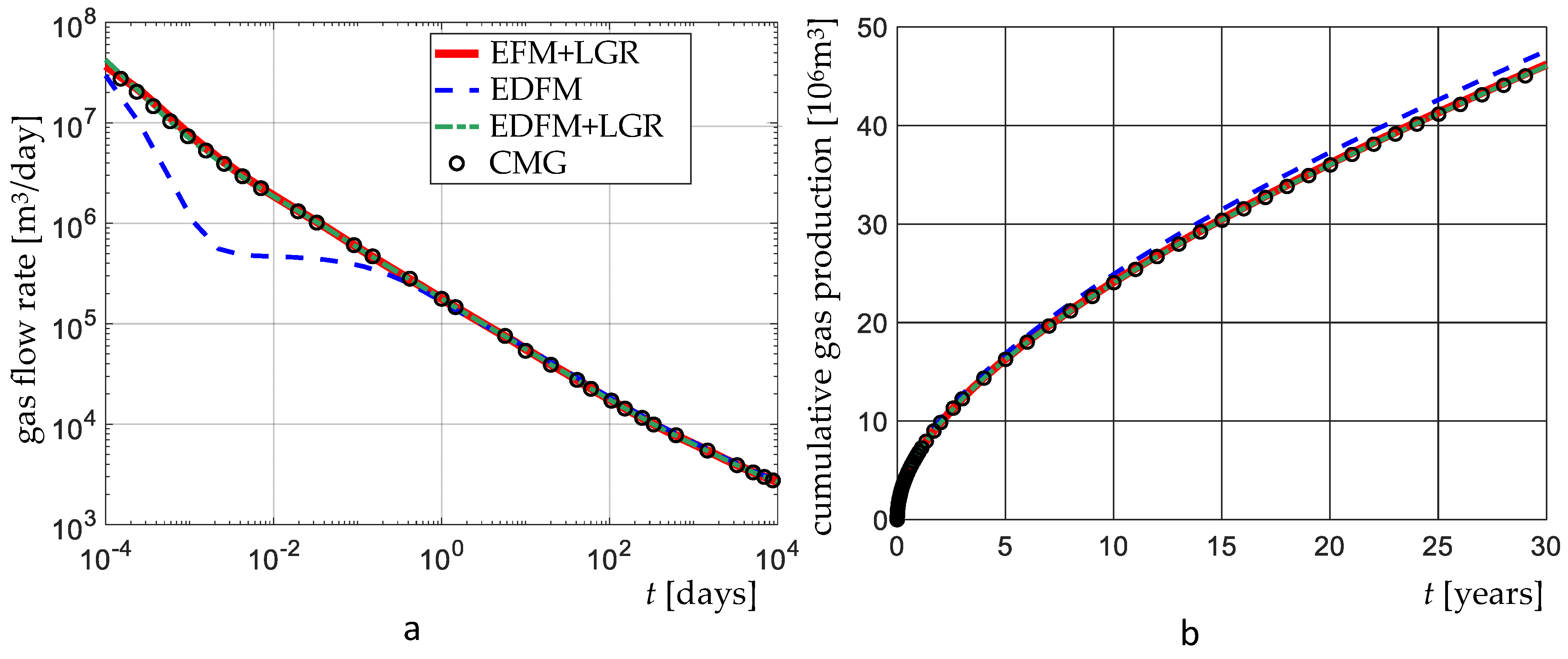
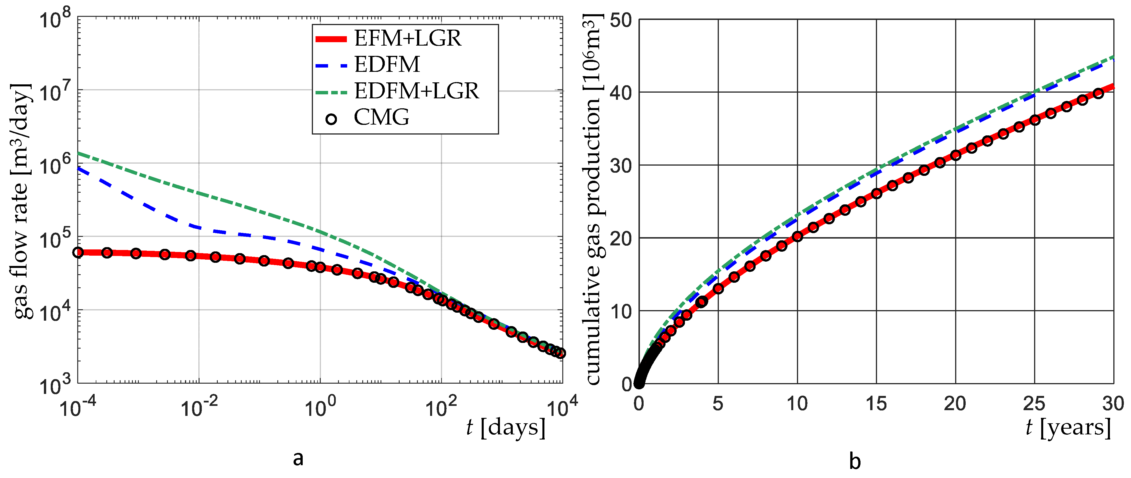
4.1. Comparison with the Commercial Simulator
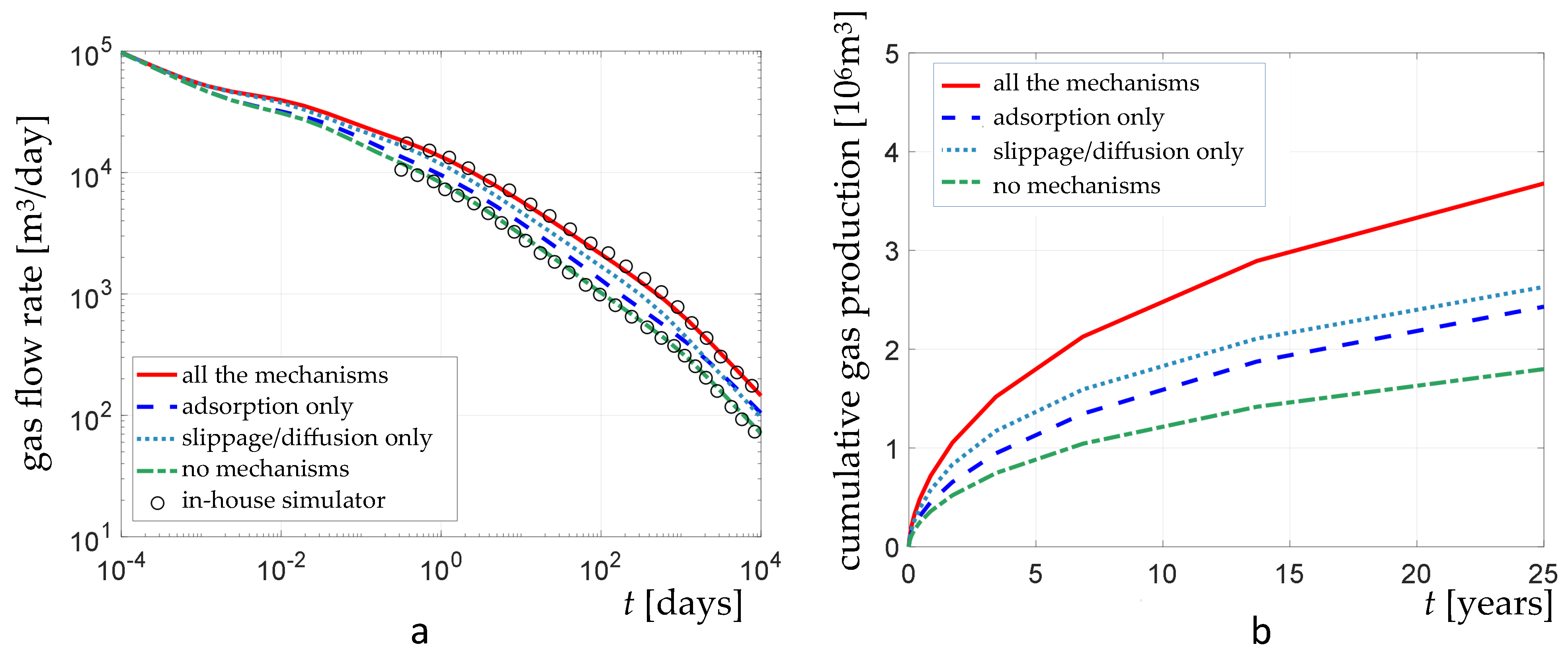
4.2. Comparison with an In-House Simulator
5. Application Examples
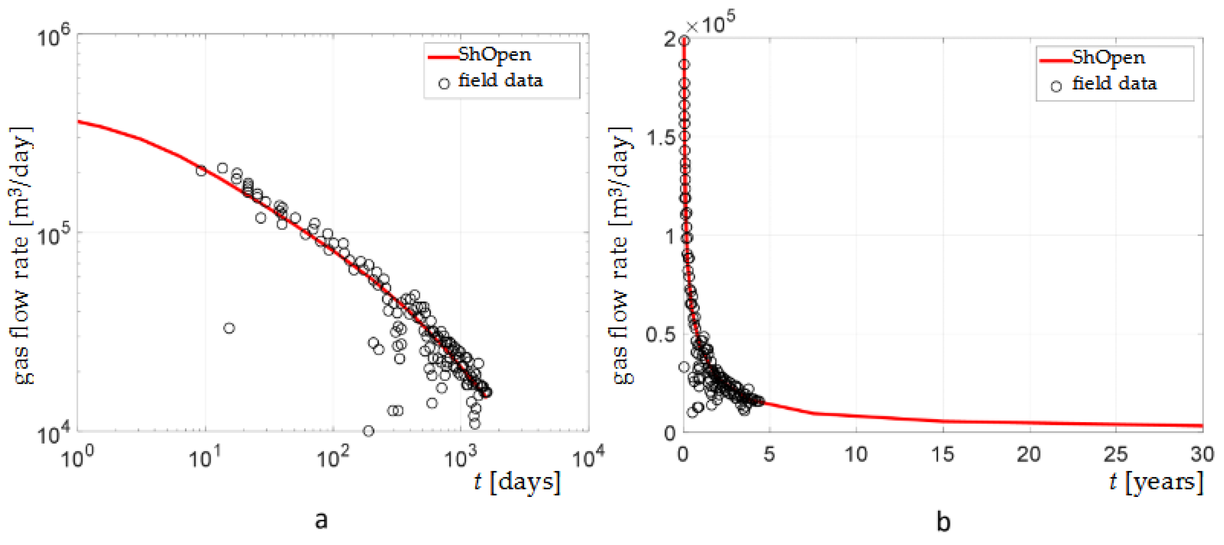
5.1. Barnett Shale Reservoir
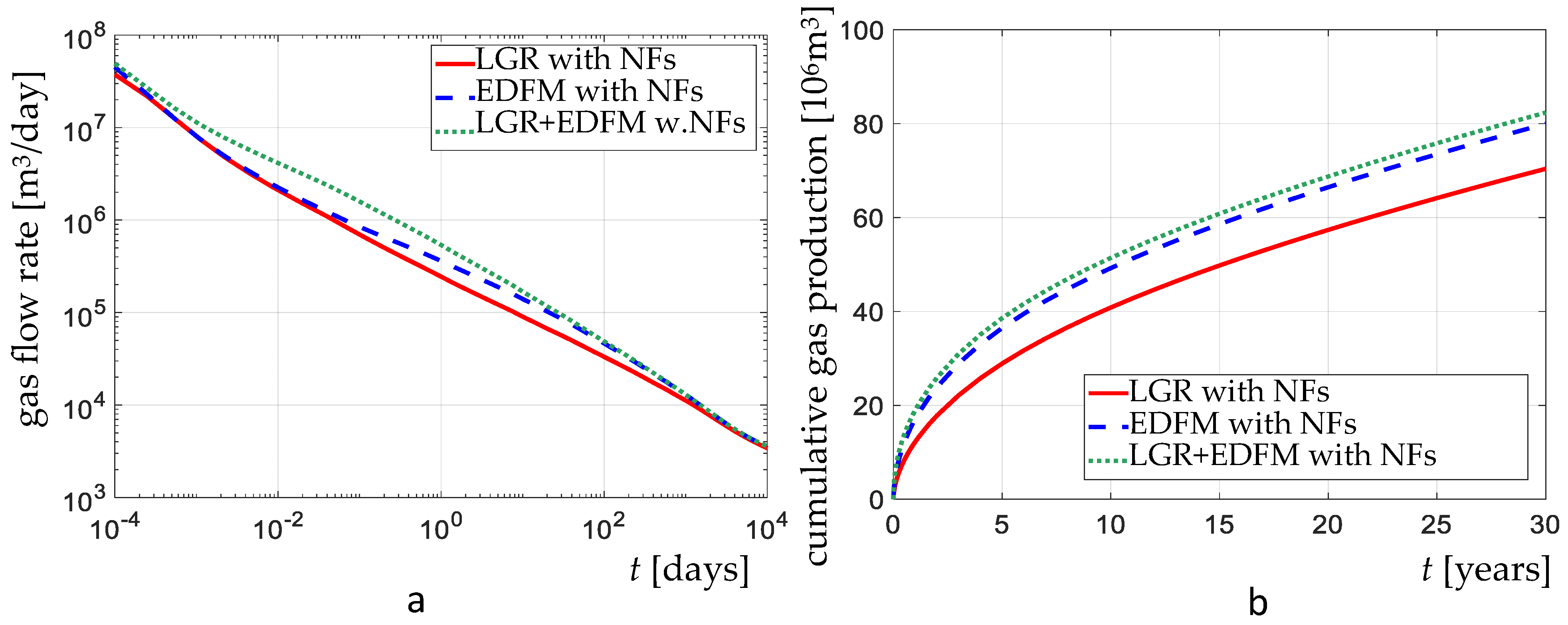
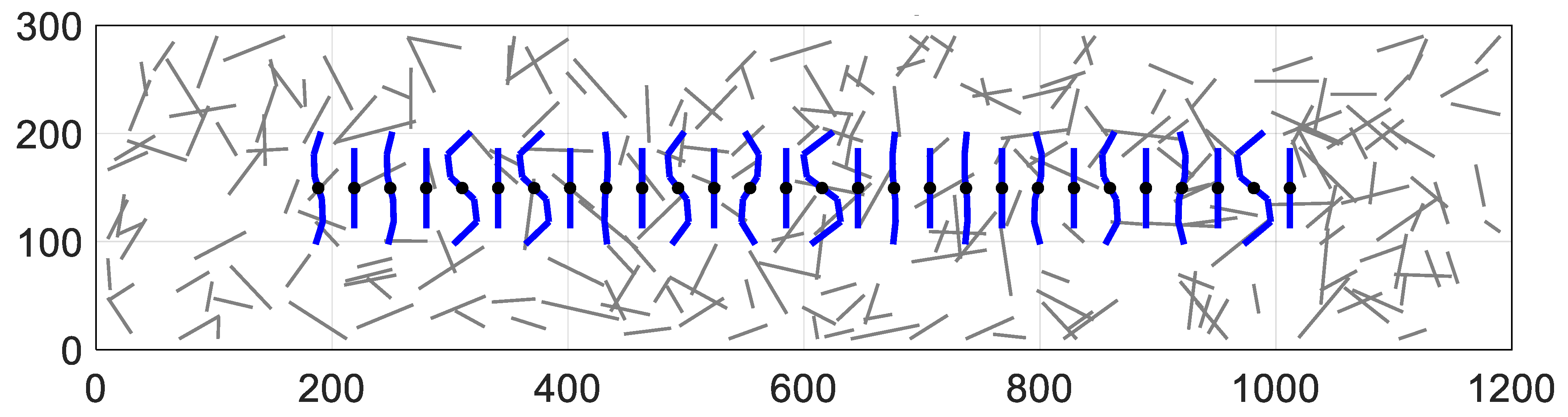
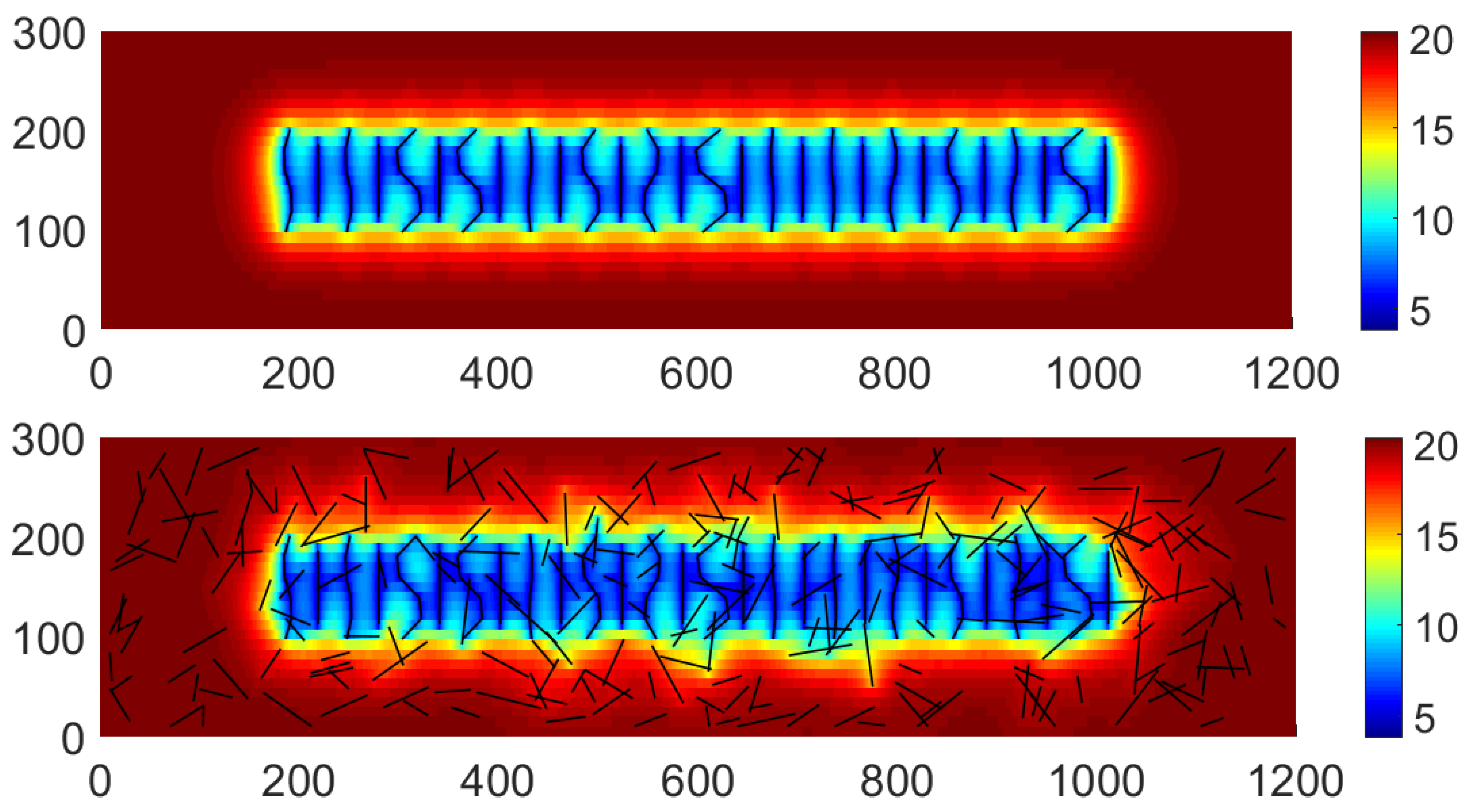
5.2. Reservoir with a Stochastic DFN
6. Conclusions
- the algorithms of the code refer to gas adsorption, gas slippage and diffusion, non-Darcy flow, and hydromechanical coupling;
- with the aid of EDFM, automatic differentiation, and a modular-designed framework, the use of ShOpen can be extended to shale gas reservoirs with embedded natural and/or artificial fractures of arbitrary fracture geometries and mutual connections;
- EDFM algorithms, implemented in ShOpen, can efficiently and accurately model stochastic DFNs, however, when dealing with low-permeability (natural) fractures and hydraulic fractures with strong gradients in the near-field, substantial errors are experienced, thus, the resort to LGR and an improved EDFM algorithm [30] are recommended;
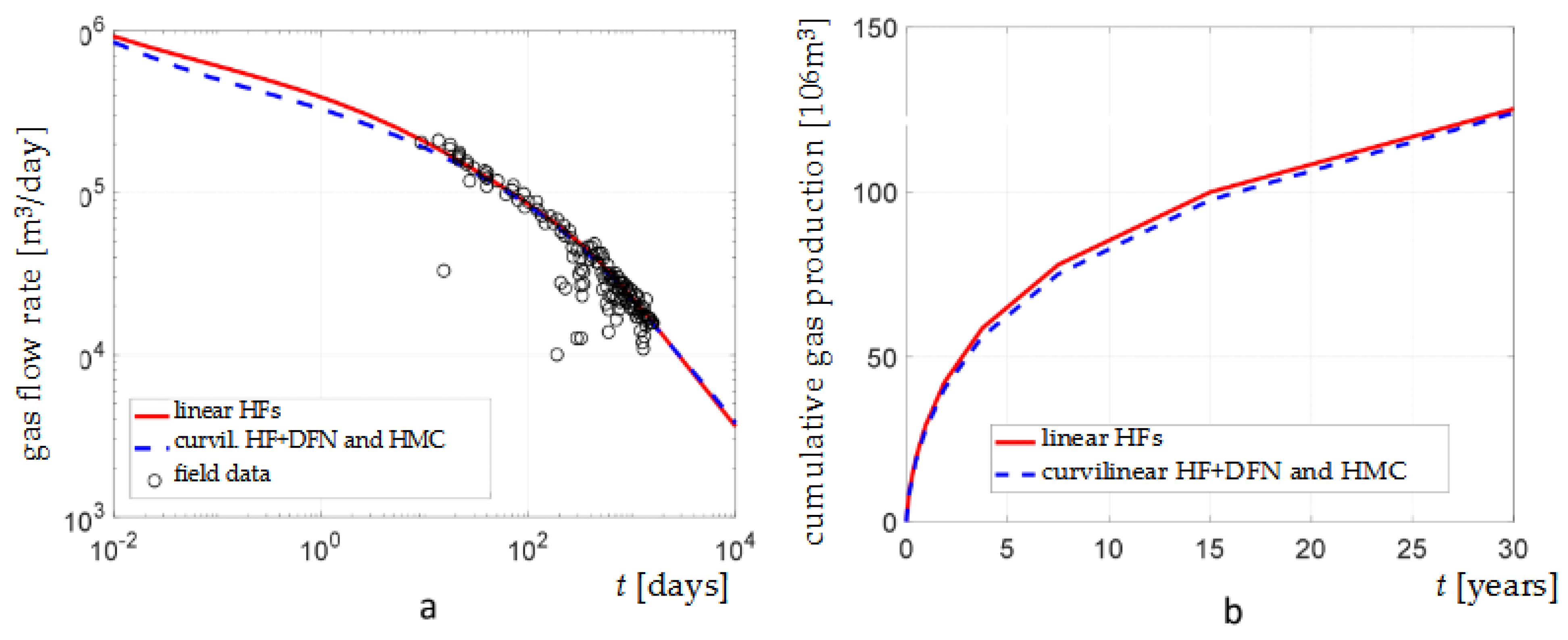
- shale gas adsorption and transport mechanisms have a significant impact on well performance; less dramatic is the impact of HM coupling and the complexity of the DFN;
- ShOpen is an efficient and flexible tool for research investigations and practical applications for the implementation of nonlinearities and the fast handling of fracture networks.
Author Contributions
Funding
Acknowledgments
Conflicts of Interest
References
- Bowker, K. Barnett Shale gas production, Fort Worth Basin: Issues and discussion. AAPG Bull. 2007, 91, 523–533. [Google Scholar] [CrossRef]
- Akkutlu, I.Y.; Efendiev, Y.; Vasilyeva, M.; Wang, Y. Multiscale model reduction for shale gas transport in poroelastic fractured media. J. Comput. Phys. 2018, 353, 356–376. [Google Scholar] [CrossRef]
- Gensterblum, Y.; Ghanizadeh, A.; Cuss, R.J.; Amann-Hildenbrand, A.; Krooss, B.M.; Clarkson, C.R.; Harrington, J.F.; Zoback, M.D. Gas transport and storage capacity in shale gas reservoirs—A review. Part A: Transport processes. J. Unconv. Oil Gas Resour. 2015, 12, 87–122. [Google Scholar] [CrossRef]
- Chen, L.; Jiang, Z.; Liu, K.; Gao, F. Quantitative characterization of micropore structure for organic-rich Lower Silurian shale in the Upper Yangtze Platform, South China: Implications for shale gas adsorption capacity. Adv. Geo-Energy Res. 2017, 1, 112–123. [Google Scholar] [CrossRef]
- Gringarten, A.C.; Ramey, H.J.; Raghavan, R. Unsteady-state pressure distributions created by a well with a single infinite-conductivity vertical fracture. Soc. Pet. Eng. J. 1974, 14, 347–360. [Google Scholar] [CrossRef]
- Cinco Ley, H.; Samaniego, F.; Dominguez, A.N. Transient pressure behavior for a well with a finite-conductivity vertical fracture. Soc. Pet. Eng. J. 1976, 18, 253–264. [Google Scholar] [CrossRef]
- Zuo, L.; Yu, W.; Wu, K. A fractional decline curve analysis model for shale gas reservoirs. Int. J. Coal Geol. 2016, 163, 140–148. [Google Scholar] [CrossRef]
- Yu, W.; Wu, K.; Sepehrnoori, K.; Xu, W. A comprehensive model for simulation of gas transport in shale formation with complex hydraulic-fracture geometry. Soc. Pet. Eng. J. 2017, 20. [Google Scholar] [CrossRef]
- Chen, Z.; Liao, X.; Sepehrnoori, K.; Yu, W. A semianalytical model for pressure-transient analysis of fractured wells in unconventional plays with arbitrarily distributed discrete fractures. Soc. Pet. Eng. J. 2018, 23. [Google Scholar] [CrossRef]
- Li, Y.; Zuo, L.; Yu, W.; Chen, Y. A fully three dimensional semi-analytical model for shale gas reservoirs with hydraulic fractures. Energies 2018, 11, 436. [Google Scholar] [CrossRef]
- Wang, B.; Feng, Y.; Du, J.; Wang, Y.; Wang, S.; Yang, R. An embedded grid-free approach for near-wellbore streamline simulation. SPE J. 2018, 23, 567–588. [Google Scholar] [CrossRef]
- Wang, B.; Feng, Y.; Pieraccini, S.; Scialò, S.; Fidelibus, C. Iterative coupling algorithms for large multidomain problems with the boundary element method. Int. J. Numer. Methods Eng. 2019, 117, 1–14. [Google Scholar] [CrossRef]
- Chen, Z.; Liao, X.; Zhao, X.; Dou, X.; Zhu, L. Performance of horizontal wells with fracture networks in shale gas formation. J. Pet. Sci. Eng. 2015, 133, 646–664. [Google Scholar] [CrossRef]
- Chen, Z.; Liao, X.; Zhao, X.; Lv, S.; Zhu, L. A semianalytical approach for obtaining type curves of multiple-fractured horizontal wells with secondary-fracture networks. SPE J. 2016, 21, 538–549. [Google Scholar] [CrossRef]
- Olorode, O.M.; Akkutlu, I.Y.; Efendiev, Y. Compositional reservoir-flow simulation for organic-rich gas shale. Soc. Pet. Eng. J. 2017, 22. [Google Scholar] [CrossRef]
- Cipolla, C.; Lolon, E.; Erdle, J.; Rubin, B. Reservoir modeling in shale-gas reservoirs. SPE Reserv. Eval. Eng. 2013, 13, 638–653. [Google Scholar] [CrossRef]
- de Dreuzy, J.R.; Davy, P.; Bour, O. Hydraulic properties of two-dimensional random fracture networks following power-law distributions of length and aperture. Water Resour. Res. 2002, 38, 12-1–12-9. [Google Scholar] [CrossRef]
- Lee, S.H.; Lough, M.F.; Jensen, C.L. Hierarchical modeling of flow in naturally fractured formations with multiple length scales. Water Resour. Res. 2001, 37, 443–455. [Google Scholar] [CrossRef]
- Karimi-Fard, M.; Gong, B.; Durlofsky, L.J. Generation of coarse-scale continuum flow models from detailed fracture characterizations. Water Resour. Res. 2006, 42. [Google Scholar] [CrossRef]
- Karimi-Fard, M.; Durlofsky, L. A general gridding, discretization, and coarsening methodology for modeling flow in porous formations with discrete geological features. Adv. Water Resour. 2016, 96, 354–372. [Google Scholar] [CrossRef]
- Miao, J.; Yu, W.; Xia, Z.; Zhao, W.; Xu, Y.; Sepehrnoori, K. An Easy and Fast EDFM Method for Production Simulation in Shale Reservoirs with Complex Fracture Geometry. In Proceedings of the 2nd International Discrete Fracture Network Engineering Conference, Seattle, WA, USA, 20–22 June 2018; American Rock Mechanics Association: Richardson, TX, USA, 2018. [Google Scholar]
- Xu, J.; Chen, B.; Sun, B.; Jiang, R. Flow behavior of hydraulic fractured tight formations considering Pre-Darcy flow using EDFM. Fuel 2019, 241, 1145–1163. [Google Scholar] [CrossRef]
- Xue, X.; Yang, C.; Onishi, T.; King, M.J.; Datta-Gupta, A. Modeling Hydraulically Fractured Shale Wells Using the Fast-Marching Method With Local Grid Refinements and an Embedded Discrete Fracture Model. SPE J. 2019, 24, 2590–2608. [Google Scholar] [CrossRef]
- Wan, X.; Rasouli, V.; Damjanac, B.; Yu, W.; Xie, H.; Li, N.; Rabiei, M.; Miao, J.; Liu, M. Coupling of fracture model with reservoir simulation to simulate shale gas production with complex fractures and nanopores. J. Pet. Sci. Eng. 2020, 193, 107422. [Google Scholar] [CrossRef]
- Bai, Y.; Liu, L.; Fan, W.; Sun, H.; Huang, Z.; Yao, J. Coupled compositional flow and geomechanics modeling of fractured shale oil reservoir with confined phase behavior. J. Pet. Sci. Eng. 2021, 196, 107608. [Google Scholar] [CrossRef]
- Cai, J.; Lin, D.; Singh, H.; Wei, W.; Zhou, S. Shale gas transport model in 3D fractal porous media with variable pore sizes. Mar. Pet. Geol. 2018, 98, 437–447. [Google Scholar] [CrossRef]
- Cai, J.; Lin, D.; Singh, H.; Zhou, S.; Meng, Q.; Zhang, Q. A simple permeability model for shale gas and key insights on relative importance of various transport mechanisms. Fuel 2019, 252, 210–219. [Google Scholar] [CrossRef]
- Zhang, T.; Sun, S.; Song, H. Flow mechanism and simulation approaches for shale gas reservoirs: A review. Transp. Porous Media 2019, 126, 655–681. [Google Scholar] [CrossRef]
- Ning, X.; Feng, Y.; Wang, B. Numerical simulation of channel fracturing technology in developing shale gas reservoirs. J. Nat. Gas Sci. Eng. 2020, 83, 103515. [Google Scholar] [CrossRef]
- Ţene, M.; Bosma, S.B.; Al Kobaisi, M.S.; Hajibeygi, H. Projection-based Embedded Discrete Fracture Model (pEDFM). Adv. Water Resour. 2017, 105, 205–216. [Google Scholar] [CrossRef]
- Yang, R.; Huang, Z.; Yu, W.; Li, G.; Ren, W.; Zuo, L.; Tan, X.; Sepehrnoori, K.; Tian, S.; Sheng, M. A comprehensive model for real gas transport in shale formations with complex non-planar fracture networks. Sci. Rep. 2016, 6, 36673. [Google Scholar] [CrossRef]
- Peng, D.Y.; Robinson, D.B. A new two-constant equation of state. Ind. Eng. Chem. Fundam. 1976, 15, 59–64. [Google Scholar] [CrossRef]
- Elliott, J.R.; Lira, C.T. Introductory Chemical Engineering Thermodynamics; Prentice-Hall International Series in the Physical and Chemical Engineering Sciences; Prentice Hall: Upper Saddle River, NJ, USA, 2012. [Google Scholar]
- Mahmoud, M. Development of a new correlation of gas compressibility factor (Z-factor) for high pressure gas reservoir. J. Energy Resour. Technol. 2013, 136, 012903. [Google Scholar] [CrossRef]
- Lee, A.L.; Gonzalez, M.H.; Eakin, B.E. The viscosity of natural gases. J. Pet. Technol. 1966, 18, 997–1000. [Google Scholar] [CrossRef]
- Klinkenberg, L.J. The permeability of porous media to liquids and gases. In Drilling and Production Practice; American Petroleum Institute: New York, NY, USA, 1941. [Google Scholar]
- Florence, F.A.; Rushing, J.; Newsham, K.E.; Blasingame, T.A. Improved permeability prediction relations for low permeability sands. In Proceedings of the SPE Rocky Mountain Oil & Gas Technology Symposium, Denver, CO, USA, 16–18 April 2007; Society of Petroleum Engineers: Tyler, TX, USA, 2007. [Google Scholar]
- Javadpour, F.; Fisher, D.; Unsworth, M. Nanoscale gas flow in shale gas sediments. J. Can. Pet. Technol. 2007, 46. [Google Scholar] [CrossRef]
- Civan, F. Effective correlation of apparent gas permeability in tight porous media. Transp. Porous Media 2010, 82, 375–384. [Google Scholar] [CrossRef]
- Yu, W.; Sepehrnoori, K.; Patzek, T.W. Modeling gas adsorption in Marcellus shale with Langmuir and BET isotherms. Soc. Pet. Eng. J. 2016, 21, 589–600. [Google Scholar] [CrossRef]
- Shen, W.; Li, X.; Cihan, A.; Lu, X.; Liu, X. Experimental and numerical simulation of water adsorption and diffusion in shale gas reservoir rocks. Adv. Geo-Energy Res. 2019, 3, 165–174. [Google Scholar] [CrossRef]
- Zeng, Z.; Grigg, R. A criterion for non-Darcy flow in porous media. Transp. Porous Media 2006, 63, 57–69. [Google Scholar] [CrossRef]
- Barree, R.D.; Conway, M.W. Beyond beta factors: A complete model for Darcy, Forchheimer, and trans-Forchheimer flow in porous media. In Proceedings of the SPE Annual Technical Conference and Exhibition, Houston, TX, USA, 26–29 September 2004; Society of Petroleum Engineers: Tyler, TX, USA, 2004. [Google Scholar]
- Rubin, B. Accurate simulation of non-Darcy flow in stimulated fractured shale reservoirs. In Proceedings of the SPE Western Regional Meeting, Anaheim, CA, USA, 27–29 May 2010; Society of Petroleum Engineers: Tyler, TX, USA, 2010. [Google Scholar]
- Hu, X.; Wu, K.; Li, G.; Tang, J.; Shen, Z. Effect of proppant addition schedule on the proppant distribution in a straight fracture for slickwater treatment. J. Pet. Sci. Eng. 2018, 167, 110–119. [Google Scholar] [CrossRef]
- Wang, H.F. Theory of Linear Poroelasticity; Princeton University Press: Princeton, NJ, USA, 2000. [Google Scholar]
- Rutqvist, J.; Stephansson, O. The role of hydromechanical coupling in fractured rock engineering. Hydrogeol. J. 2003, 11, 7–40. [Google Scholar] [CrossRef]
- Cammarata, G.; Fidelibus, C.; Cravero, M.; Barla, G. The hydro-mechanically coupled response of rock fractures. Rock Mech. Rock Eng. 2007, 40, 41–61. [Google Scholar] [CrossRef]
- Fidelibus, C. The 2D hydro-mechanically coupled response of a rock mass with fractures via a mixed BEM–FEM technique. Int. J. Numer. Anal. Methods Geomech. 2007, 31, 1329–1348. [Google Scholar] [CrossRef]
- Hu, M.; Wang, Y.; Rutqvist, J. Fully coupled hydro-mechanical numerical manifold modeling of porous rock with dominant fractures. Acta Geotech. 2017, 12, 231–252. [Google Scholar] [CrossRef]
- Gangi, A.F. Variation of whole and fractured porous rock permeability with confining pressure. Int. J. Rock Mech. Min. Sci. Geomech. Abstr. 1978, 15, 249–257. [Google Scholar] [CrossRef]
- Shi, J.Q.; Durucan, S. Near-exponential relationship between effective stress and permeability of porous rocks revealed in Gangi’s phenomenological models and application to gas shales. Int. J. Coal Geol. 2016, 154, 111–122. [Google Scholar] [CrossRef]
- Alramahi, B.; Sundberg, M.I. Proppant embedment and conductivity of hydraulic fractures in shales. In Proceedings of the 46th ARMA US Rock Mechanics/Geomechanics Symposium, Chicago, IL, USA, 24–27 June 2012; Society of Petroleum Engineers: Tyler, TX, USA, 2012. [Google Scholar]
- Wu, W.; Zhou, J.; Kakkar, P.; Russell, R.; Sharma, M.M. An experimental study on conductivity of unpropped fractures in preserved shales. Soc. Pet. Eng. J. 2019, 34, 280–296. [Google Scholar] [CrossRef]
- Lie, K.; Krogstad, S.; Ligaarden, I.S.; Natvig, J.R.; Nilsen, H.M.; Skaflestad, B. Open-source MATLAB implementation of consistent discretisations on complex grids. Comput. Geosci. 2012, 16, 297–322. [Google Scholar] [CrossRef]
- Xu, Y. Implementation and application of the Embedded Discrete Fracture Model (EDFM) for Reservoir Simulation in Fractured Reservoirs. Master’s Thesis, The University of Texas at Austin, Austin, TX, USA, 2015. [Google Scholar]
- Ţene, M.; Al Kobaisi, M.S.; Hajibeygi, H. Algebraic multiscale method for flow in heterogeneous porous media with embedded discrete fractures (F-AMS). J. Comput. Phys. 2016, 321, 819–845. [Google Scholar] [CrossRef]
- Karimi-Fard, M.; Durlofsky, L.J.; Aziz, K. An efficient discrete fracture model applicable for general purpose reservoir simulators. In Proceedings of the SPE Reservoir Simulation Symposium, Houston, TX, USA, 3–5 February 2003; Society of Petroleum Engineers: Tyler, TX, USA, 2003. [Google Scholar]
- Jiang, J.; Younis, R.M. Numerical study of complex fracture geometries for unconventional gas reservoirs using a discrete fracture-matrix model. J. Nat. Gas Sci. Eng. 2015, 26, 1174–1186. [Google Scholar] [CrossRef]
- Cao, P.; Liu, J.; Leong, Y.K. A fully coupled multiscale shale deformation-gas transport model for the evaluation of shale gas extraction. Fuel 2016, 178, 103–117. [Google Scholar] [CrossRef]
- Fadakar Alghalandis, Y. ADFNE: Open source software for discrete fracture network engineering, two and three dimensional applications. Comput. Geosci. 2017, 102, 1–11. [Google Scholar] [CrossRef]


| Analytical | Semianalytical | Structured Grid | Unstructured Grid | EDFM | |
|---|---|---|---|---|---|
| accuracy | ++ | ++ | +++ | +++ | ++ |
| handling nonlinear mechanisms | + | + | +++ | +++ | +++ |
| handling rock heterogeneity | + | + | +++ | +++ | +++ |
| quality of DFN mesh | +++ | +++ | + | + | +++ |
| preprocessing efficiency | +++ | +++ | +++ | +++ | ++ |
| computational efficiency | +++ | +++ | + | ++ | ++ |
| Mechanism | Model | Type | Domain |
|---|---|---|---|
| adsorption | Langmuir, BET | A | matrix |
| slip flow/diffusion | Klinkenberg [36], Florence et al. [37], Javadpour et al. [38], Civan [39] | T | matrix |
| non-Darcy flow | Darcy–Forchheimer | T | fracture |
| Property | Unit | Value |
|---|---|---|
| domain dimensions | m | 606.6 × 606.6 |
| formation thickness | m | 45.72 |
| initial reservoir pressure | MPa | 34.47 |
| reservoir temperature T | K | 327.60 |
| Langmuir pressure | MPa | 8.96 |
| Langmuir volume | m/kg | 0.0041 |
| matrix porosity | - | 0.07 |
| matrix compressibility | 1/Pa | 1.45 × 10 |
| matrix permeability | nD | 500 |
| fracture permeability | mD | 0.5–1000 |
| fracture width w | m | 0.003 |
| fracture half-length ½ | m | 106.68 |
| fracture conductivity | mD-ft | 5–10,000 |
| well BHP | MPa | 3.45 |
| Property | Unit | Value |
|---|---|---|
| domain dimensions | m | 200,140 |
| formation thickness | m | 10 |
| initial reservoir pressure | MPa | 16 |
| reservoir temperature T | K | 343.15 |
| Langmuir pressure | MPa | 4 |
| Langmuir volume | m/kg | 0.018 |
| matrix porosity | - | 0.1 |
| matrix compressibility | 1/Pa | 1.0 × |
| matrix permeability | nD | 100 |
| fracture porosity | - | 1.0 |
| fracture permeability | D | 1 |
| fracture width w | m | 1× |
| well BHP | MPa | 4 |
| wellbore skin factor s | - | 43 |
| Property | Unit | Value |
|---|---|---|
| domain dimensions | m | 1200,300 |
| formation thickness | m | 90 |
| initial reservoir pressure | MPa | 20.34 |
| reservoir temperature T | K | 352 |
| rock density | kg/m | 2500 |
| Langmuir pressure | MPa | 4.47 |
| Langmuir volume | m/kg | 0.00272 |
| matrix porosity | - | 0.1 |
| matrix compressibility | 1/Pa | 1.0 × |
| matrix permeability | nD | 200 |
| fracture porosity | - | 0.03 |
| fracture permeability | D | 1.0 × |
| fracture width w | m | 0.003 |
| fracture half-length ½ | m | 47.2 |
| fracture conductivity | mD-ft | 1 |
| well bottom-hole pressure BHP | MPa | 3.69 |
| wellbore skin factor s | - | 19 |
| Property | Unit | Value |
|---|---|---|
| Biot coefficient | - | 0.5 |
| overburden stress | MPa | 38 |
| maximum horizontal stress | MPa | 34 |
| minimum horizontal stress | MPa | 29 |
| effective modulus of the asperities | MPa | 180 |
| Gangi exponential constant m | - | 0.5 |
| N fracture permeability | mD | 10 |
Publisher’s Note: MDPI stays neutral with regard to jurisdictional claims in published maps and institutional affiliations. |
© 2021 by the authors. Licensee MDPI, Basel, Switzerland. This article is an open access article distributed under the terms and conditions of the Creative Commons Attribution (CC BY) license (http://creativecommons.org/licenses/by/4.0/).
Share and Cite
Wang, B.; Fidelibus, C. An Open-Source Code for Fluid Flow Simulations in Unconventional Fractured Reservoirs. Geosciences 2021, 11, 106. https://doi.org/10.3390/geosciences11020106
Wang B, Fidelibus C. An Open-Source Code for Fluid Flow Simulations in Unconventional Fractured Reservoirs. Geosciences. 2021; 11(2):106. https://doi.org/10.3390/geosciences11020106
Chicago/Turabian StyleWang, Bin, and Corrado Fidelibus. 2021. "An Open-Source Code for Fluid Flow Simulations in Unconventional Fractured Reservoirs" Geosciences 11, no. 2: 106. https://doi.org/10.3390/geosciences11020106
APA StyleWang, B., & Fidelibus, C. (2021). An Open-Source Code for Fluid Flow Simulations in Unconventional Fractured Reservoirs. Geosciences, 11(2), 106. https://doi.org/10.3390/geosciences11020106