Abstract
Recent achievement of research on soil-structure interaction (SSI) is reviewed, with a main focus on the numerical analysis. The review is based on the continuum mechanics theory and the use of high-performance computing (HPC) and clarifies the characteristics of a wide range of treatment of SSI from a simplified model to a high fidelity model. Emphasized is that all the treatment can be regarded as the result of the mathematical approximations in solving a physical continuum mechanics problem of a soil-structure system. The use of HPC is inevitable if we need to obtain a solution of higher accuracy and finer resolution. An example of using HPC for the analysis of SSI is presented.
1. Introduction
Research related to the effects of soil-structure interaction (SSI) on structural seismic response has been a key issue in earthquake engineering for several decades. Numerous articles on SSI, which included extensive review papers, were published; see [1,2,3,4] in the early days of earthquake engineering. Regarding numerical analysis that uses finite element method (FEM) for the evaluation of SSI, the most influential work is Wolf [5].
In this review paper, we aim at summarizing recent advancements in numerical analysis related to SSI. To this end, we consider the following two fundamentals: (1) the continuum mechanics theory on which most rigorous treatment of SSI is made and (2) the use of high-performance computing (HPC) for large-scale seismic response analysis considering SSI. These two fundamentals are related to each other because the continuum mechanics theory leads to the governing equations for SSI which are given as a set of four-dimensional partial differential equations for the three components of a displacement vector function and the set cannot be numerically solved without using modern computers of fast CPU’s (Central Processing Unit) and large computing memories. A soil-structure system of 100 m dimension would need an analysis model of 106~9 degree-of-freedom (DOF) if the spatial resolution is 1~0.1 m and the duration of 10~100 s would need 104~5 time steps if the temporal resolution is 0.01 s.
When computers were slow and could not solve problems of 1,000,000 DOF, we had to approximate the governing equation that was derived from the continuum mechanics theory to obtain an approximate solution of the governing equation. We dare say that structural mechanics theory for beam, plate or shell can be regarded as a sophisticated approximation of the continuum mechanics theory and an approximate theory can provide an approximate but accurate solution to the original continuum mechanics problem using a computer of limited performance. As for SSI, however, such an approximate but accurate solution could not be easily obtained because developing approximate treatment of soil was much more difficult than developing approximate treatment of structures. For instance, a set of soil-springs are the simplest approximate treatment of soil. This treatment works well for certain conditions but the applicability of this treatment is much more limited than the applicability of the beam, plate or shell theory for structures.
Based on the two fundamentals of the continuum mechanics theory and the use of HPC, we will review a methodology for numerically evaluating SSI. The progress of computer hardware and software is fast and the use of computers of higher performance will be an ordinary practice for solving larger scale problems DOF of which exceeds 1,000,000 or 10,000,000. Moreover, the cost for numerical computation is decreasing; computers and programs are available for the evaluation of SSI. We thus emphasize the significance of understating the mechanism of SSI from the viewpoint of the continuum mechanics theory and correctly computing the effects of SSI using an analysis model of high fidelity for a soil-structure system.
The contents of this review paper are as follows. Firstly, we review past review articles on SSI, focusing on the numerical study. Secondly, we present the most rigorous treatment of SSI based on the continuum mechanics theory. We present an interpretation of the ordinary treatment of SSI as a mathematical approximation of the rigorous treatment. Thirdly, we provide an example of using FEM enhanced with HPC for evaluating SSI by using a large-scale analysis model. We point out future works that are needed for further understanding and numerical analysis of SSI.
2. Literature Survey on Evaluation of SSI
The change in the dynamic response of the structure because of the presence of underlying soil and vice versa is called SSI. There are two aspects of SSI. The first is the modification of the free-field ground motion due to the presence of the structure and the second is the modification of the structural response due to the flexibility of the supporting soil. In the case of flexible structures founded on rigid ground, the effect of SSI on the structural response is not significant; and it has been ignored in the conventional structural analysis. For stiff and heavy structures, the soil flexibility can change the structural response significantly and ignoring SSI can lead to unsafe design [6]. This is the major target of evaluating the effects of SSI.
SSI was studied in the early twentieth century and it was found that the effects of SSI could influence structural seismic response and ought to be taken into consideration for the seismic resistance design. Observations made during large earthquakes in the past emphasized the need to correctly evaluate the effects of SSI on the seismic response analysis. The difficulty of evaluating the effects of SSI is the dependence of SSI on the characteristics of both the structure and the soil. As mentioned, the effects of SSI tend to be more significant for the case of heavy and stiff structures founded on weaker soils. The characteristics of input ground motion influence the effects of SSI on the structural seismic response as well. However, this influence is often overlooked.
The first attempt to study the phenomenon of SSI was made in Japan by Sezawa and Kanai in 1935 [7,8]. The theory of SSI was properly developed for the first time by Reissner, who studied the behavior of a circular foundation lying on an elastic half-space and subjected to vertical time-harmonic loading, in 1936 [9]. Since then, numerous analytical and numerical research studies have been conducted on the evaluation of SSI for a more accurate seismic response analysis; some recent studies are [10,11,12,13,14]. Several experimental works involving full or reduced scale tests of SSI problem have also been conducted during this period; see [15,16,17,18].
In general, two approaches are used for evaluating the effects of SSI. The first approach is the direct method in which the structure and soil are modeled and their response is solved simultaneously by carrying out the time integration of governing equations of the structure and soil models. The second approach is the substructure method (or the indirect method) in which the structure and soil are separated by introducing a rigid interface between them and their responses are solved individually in the frequency domain. A key issue of the substructure method is the dynamic impedances for the soil domain which is modeled as a spring and a dashpot.
2.1. Direct Method for Evaluating SSI
In the direct method, the structure and soil are considered as a system and an analysis model for them is constructed. A suitable governing equation is posed for the structure and soil and the finite element method (FEM) is used to solve the equation in the time domain. This approach is conceptually simple. The direct method involves the non-linear numerical analysis of a high-fidelity model of the structure which is constructed from three-dimensional geometry of the structure. However, it is often the case that some physical assumptions are made in posing the governing equation, such as the application of two-dimensional model and the application of the structural element models. Making physical assumptions is always acceptable with a condition that the assumptions made ought to be validated by the experiments or the observation.
A key issue of the direct method is the determination of the dimension (or size) of the soil domain and the artificial boundary conditions on the side surfaces of the soil domain. They are essential for accurately simulating the effect of the surrounding soil as well as to avoid the trapping of waves reflected from the structure inside the soil domain. For this reason, a standard option is to use a sufficiently large dimension for the soil domain so that the wave reflected from the structure is dissipated before reaching the boundary. Several studies were made to develop suitable artificial boundary conditions to reduce the dimension of the soil domain. The representative artificial boundary conditions are the introduction of the viscous boundary, consistent boundary, unified boundary, transmitting boundary, periodic boundary and the viscous spring boundary; see [19,20,21,22,23,24]. These boundary conditions act either as non-reflecting boundaries or as adsorbing layers, in order to avoid the reflections of the outward propagating waves from the soil domain.
Despite the presence of artificial boundaries, the direct method requires an analysis model of a significant volume of the soil domain for the accurate evaluation of SSI. Such an analysis model becomes significantly large if the shear wave velocity is 100 m/s and the temporal resolution is 0.1 s, the wavelength of the shear wave is 10 m and we need the spatial resolution of 1 m to accurately compute this wave. As finer temporal resolution (or responses in higher frequency) is required, the time increment, as well as the element size, decreases accordingly, which results in an analysis model of larger DOF and a larger number of time steps. For this reason, the direct approach with three-dimensional high-fidelity models has not been often used. With the advancement of computers, the works applying larger three-dimensional models have been increasing; see [25,26,27,28]. The characteristic of such works is that they applied the solid element models with non-linear property only to the soil domain, not to the structure domain. Recently, computational techniques enable us to apply the direct method for the evaluation of SSI, which includes the non-linear numerical analysis of a high fidelity model of a soil-structure system; see [29,30,31]. Still, the governing equation and the analysis model are simplified to obtain an approximate solution, by making certain physical assumptions for material properties of soil and concrete.
2.2. Substructure Method for Evaluation of SSI
In the substructure method, the structure and soil are considered separately; it is assumed that a rigid body foundation is put between the structure and soil. In this method, the seismic response analysis takes the following three steps: (1) the determination of the input ground motion, which is different from the free field ground motion due to the presence of the structure (termed as kinematic interaction); (2) the determination of the frequency dependent impedance functions for the foundation, by giving a unit harmonic excitation of displacement/rotation at a particular frequency to the foundation, computing the reactional force/moment of the soil and computing the ratio of the input and the reaction as an impedance function; and (3) the calculation of the dynamic response of the structure supported by the springs with the impedance functions determined in the second step, subjected to the input motion determined in the first step (termed as inertial interaction).
As for the determination of the input ground motion, analytical solutions were found in the substructure method for the cases of a structure and a half-space of soil with simple configuration and material properties. Research was carried out for a surface foundation and a piled or embedded foundation. A one-dimensional analysis that assumes uniform or stratified ground structure(s) and the vertical propagation of shear waves is used for the evaluation. Kinematic interaction is the lack of match of the foundation with the free field ground motion. It occurs because of the difference in foundation stiffness from that of the surrounding ground which causes reflection and refraction of the seismic waves approaching the soil foundation interface. For the case of the surface foundation, the kinematic interaction is ignored since it is assumed that only shear waves propagate in the vertical direction; as explained later, the presence of the structure locally influences the shear waves because the traction free boundary conditions on the ground surface are not satisfied on the bottom of the structure even though its weight is regarded as the force on the vertical direction. However, for the case of a stiff embedded foundation, the free field input ground motion is modified resulting in rotational motion for the foundation.
As for the determination of the frequency-dependent impedance functions, the mathematical problem of the soil domain is formulated as a mixed boundary value problem. Several analytical or empirical solutions were found for this problem; for instance, see [32,33,34,35,36] for the analytical solutions and [37] for the empirical solutions. These solutions were applied to model the soil domain as sway-rocking spring for a range of structures; see [38,39,40,41,42], as well as to develop numerical analysis programs such as CLASSI [43], FLUSH [44] and SASSI [45]. Further extending this approach, several more complex models, termed as lumped parameter models for SSI analysis, are also developed; see [46,47,48].
It should be noted that the applicability of these solutions is limited to determine the frequency-dependent impedance functions. This is because the solutions are for a simple circular or rectangular rigid foundation which is perfectly bonded to a homogeneous half space of linearly isotropic elasticity subjected to the excitation at the centroid of the foundation. The solutions could be used for a soil-structure system that is similar to the ideally simplified model. There were studies that showed significant differences between the observed data and the solutions that were synthesized by using the analytical solutions [49].
Other than the two basic approaches as mentioned above, a third hybrid approach based on macro-elements has also been developed recently. This approach combines the features of the substructure approach, that is, domain decomposition and finite element modeling. The soil and foundation system is replaced by a single element termed as macro-element located at the foundation level. The major assumption for this approach is also the same as for substructure approach, that is, the presence of the rigid body at foundation level. The first macro element was proposed by Nova & Montrasio [50] for a simplified case of footing and soil subjected to monotonic loading. Since then several macro element models have been proposed with different loading scenarios, foundation shapes and soil types; see for instance [51,52,53,54,55].
We have to point out that the frequency domain analysis of a structure is smart in the sense that it considerably reduces the numerical computation for the structural responses which are mainly governed by a few first modes. However, dynamic responses of three-dimensional grounds are different from the structures and the decomposition of the responses in the time domain is much more complicated; the use of a stratified ground model provides a clear perspective to the soil behavior but it might lead to over-simplifications compared with simplifications of structural modal analysis.
It should also be noted that while the applicability is limited, the use of simplified models of the soil domain is needed at the initial stages of numerical analysis to obtain overall soil responses or for the seismic probabilistic risk analysis which needs only rough estimates of ground motion amplification. In order to link the substructure method that uses a simplified model and the direct method that uses a high fidelity model, we have to maintain the consistency of the simplified model, that is, solving the same physical problem with different degrees of mathematical approximations. Losing the consistency would be fatal because it is impossible to evaluate the accuracy of the solution. Comparison with observed data is a straightforward way to examine the accuracy of the numerical analysis and it is easy for a simplified model to reproduce observed data by tuning a few parameters of the model. For the prediction, however, we have to understand the limitation of using the simplified model.
The co-existence of the conventional simplified model and the high fidelity model causes some confusion about the numerical analysis of evaluating the effects of SSI on the structural seismic responses; these two groups of the analysis models are constructed for solving different mathematical problems and hence it appears that the different mathematical problems correspond to different physical problems; see [56]. As shown in the next section, however, the continuum mechanics theory provides a single physical problem for a soil-structure system which is expressed in the form of a functional (or a Lagrangian) and various mathematical problems are derived from the functional by making suitable mathematical approximations. Unlike the physical assumptions which need to be validated by the experiments or the observation, we do not have to validate mathematical approximations. Instead, we examine the accuracy of the solutions which are obtained by solving the mathematically approximated problem with the exact solution. It should be noted that each mathematically approximated problem has its own exact solution but that exact solution is regarded as an approximate solution for the original problem which is not mathematically approximated.
3. Analysis of SSI Based on Continuum Mechanics Theory
The continuum mechanics theory, which is based on Newtonian mechanics, can predict mechanical behaviors of solid or fluid if its size is much larger than molecules or atoms that constitute the body. As mentioned, this theory leads to a set of coupled four-dimensional partial differential equations as the governing equation of the mechanical behavior, which cannot be solved without using modern fast and large computers. The governing equation is simple since it does not include terms of interactions. Indeed, the differential equations are for the temporal and spatial derivatives of a displacement function at one point and one instance and terms related to other points or times are not included. However, the interaction between one part and the other part of the body or between a certain time and other times are accurately evaluated by solving the differential equations; we should recall that Newton’s second law is expressed in the form of a temporal differential equation, which is prescribed for each instance and does not include terms of the past or future. According to the continuum mechanics theory, therefore, the accurate evaluation of SSI is made just by solving the governing equation accurately, provided that initial and boundary conditions, as well as the configuration and material properties of the body, are prescribed accurately.
Based on the continuum mechanics theory, it is readily proved that some structural mechanics theories are a mathematical approximation of the continuum mechanics theory; see [57]. For instance, a beam theory which uses only Young’s modulus and neglects Poisson’s ratio is rigorously derived from the linear isotropic elasticity of the continuum mechanic theory (that uses both Young’s modulus and Poisson’s ratio) by making suitable mathematical approximations; an assumption of a one-dimensional stress-strain relation via Young’s modulus is not needed. A plate theory is derived from the continuum mechanics theory in the same manner, that is, by making mathematical approximations.
The derivation of the continuum mechanics theory to structural mechanics theory uses a Lagrangian of the continuum. If a suitable Lagrangian is given to a system of a structure and soil, it can yield a wide range of mathematical problems; the most rigorous problem is to the variational problem of the Lagrangian without making any mathematical approximations and the simplest problem results in a mass spring system. The mathematical problems derived from the Lagrangian are different due to the difference in the mathematical approximations. Still, these problems are consistent since they provide approximate solutions to the common problem of the Lagrangian. For the simplified modeling, the consistency to the original continuum mechanics problem is of essential importance.
Using the Lagrangian, we show that the conventional soil-spring model can be objectively constructed from it, by applying mathematical approximations to displacement functions. No physical assumptions should be made in constructing the soil-spring model to maintain consistency with the original continuum mechanics problem.
3.1. Lagrangian of SSI
As the simplest example, we consider a linearly elastic body. A Lagrangian is formulated for a system of a structure and soil; it is a functional for a displacement function. The wave equation is derived from the Lagrangian as the governing equation for the displacement function when no mathematical approximations are made. Another governing equation can be derived from the Lagrangian when a displacement function of a particular form, which is regarded as a mathematical approximation, is used.
To formulate the Lagrangian, we denote a structure and soil by and , respectively; is regarded as a finite region where ground motion is input at the bottom surface and suitable absorbing boundary conditions are posed at the side surfaces; see Figure 1. Assuming infinitesimally small deformation, we define the following Lagrangian for a displacement function, :
where and are density and elasticity, and stand for the temporal and spatial derivative of and and are inner product and second-order contraction, respectively; a bold character is used for a vector or tensor quantity. The Lagrangian problem of yields
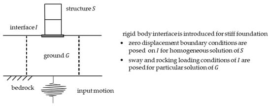
Figure 1.
Schematic view of structure and ground.
This is the wave equation or the governing equation for . As is seen, Equation (2) does not have any terms for SSI in it. Still, the solution of Equation (2) accounts for the effects of SSI on the structural responses.
Now, we consider suitable mathematical approximations for , paying attention to the condition on the interface between and , denoted by . The conventional analysis of SSI usually assumes that is an infinitesimally thin and rigid body plate. The restriction ought to enforce the continuity of displacement and traction across ; see Appendix A.
3.2. Consistent Mass Spring Model Accounting for SSI
As the first step of reducing an HPC model, we study the case when a displacement function is described only in and a displacement function in is ignored. We consider the following displacement function:
where is a one-directional horizontal input ground motion on , is a constant vector field the direction of which is parallel to the one-directional input ground motion and is the first mode of the structure, satisfying in , with being the natural frequency of the first mode. Substitution of Equation (3) into of Equation (1) yields
where and are defined as and . For this of Equation (4), leads to
By posing suitable initial conditions for unknown , we can uniquely obtain .
Equation (5) coincides with the governing equation of a mass spring model; see Figure 2. By definition, and satisfy . Thus, the mass spring model has the natural frequency of the structure, . Note that is set to satisfy , where is a suitable point of and that makes equal the total mass of . Therefore, if satisfies
then, that is computed by solving Equation (4) is an approximate solution of the displacement at .

Figure 2.
Mass spring model without soil spring.
3.3. Consistent Mass Spring System with Sway Spring Accounting for SSI
As the next step, we consider the following displacement function described in and :
where is the translation of , is the displacement field in caused by the one-directional input ground motion in the absence of and is the displacement function in induced by on . Substitution of Equation (7) into of Equation (1) yields
where and . For this of Equation (8), leads to
By posing suitable initial conditions for unknown and , we can uniquely obtain and .
Equation (9) coincides with the governing equation of a mass spring model with a sway spring; which has the mass, the spring constant and the sway spring constant of , and , respectively, if
is satisfied together with Equation (6). Indeed, Equation (9) becomes
which is the governing equation of the mass spring system with the sway spring with the mass and the spring constant being and and the sway spring constant being ; see Figure 3.

Figure 3.
Mass spring model with sway spring.
There are many choices of ; a harmonic loading of with any period is such a choice. varies depending on the choice of . The meta-modeling theory cannot specify a suitable choice of so that the solution of the resulting equation is not always a good approximate solution. However, the theory shows that Equation (10) is necessary for the sway spring, just as Equation (6) is needed for the mass spring model; see [58,59].
3.4. Extension of Consistent Multiple Mass Spring System Accounting for SSI
It is straightforward to construct a multiple mass spring system model. As an illustrative example, we consider a set of dynamic modes, , for and a set of harmonic translations of , , for ; is the -th mode with the natural frequency and is the displacement function of when is subjected to the harmonic translation with the frequency . We consider the following displacement function:
Substitution of Equation (12) into of Equation (1) yields
Here, for simplicity, is denoted by and is replaced by . For of Equation (13), leads to
for and the summation of is taken from .
Note that the last two terms in Equation (14b) are shared for all ’s. Since Equation (14a) gives , Equation (14b) becomes
if and are satisfied. Equation (15) is regarded as a set of the coupled equations for the sway springs.
It should be noted that sharing in Equation (14b) is the consequence of Equation (13), which includes in . It should also be noted that while these displacement functions are continuous across , they do not accompany traction functions which are continuous across ; while produces stress in , does not produce any stress in ; see Figure 4. Therefore, it is well expected that the displacement function of Equation (12) does not provide a good approximate solution for the original problem.

Figure 4.
Displacement function induced by rigid body translation of interface.
It is also straightforward to include a rocking spring in a mass spring model. For simplicity, we consider only one mode in and one function of translation and rotation of for a displacement function, that is,
where is rotation, is a linear function in and is a decaying function in ; and are the displacement functions induced by the rigid body rotation of . Substitution of Equation (16) into Equation (1) yields
where or is the integration which is taken over in a form similar to and or is the integration taken over in a form similar to and ; see Appendix B. For this of Equation (17), leads to
Equation (18) coincides with the governing equation of a mass spring model with a sway spring and a rocking spring, if
is satisfied, together with Equations (6) and (10). Indeed, Equation (18) becomes
which is the governing equation of the mass spring system with the sway and rocking springs, with the mass and the spring constant, and and the sway and rocking spring constant, and . Just like , this is defined as in terms of .
We have to emphasize that Equations (6), (10) and (19) are used in order to reduce an FE model of high fidelity to a mass spring model with sway and rocking springs. The mass spring model could be a good and simple model if these three equations are satisfied. Still, it has a limitation of applicability since the mathematical approximations for the displacement functions are required in reducing the FE model to the mass spring model.
Using a larger number of the soil-springs does not contribute to increasing the agreement by themselves. This is because the harmonic displacements, and , have coupling effects with the ground motion, (i.e., , , and ) and we have to include terms that account for the effects. These terms change depending on and hence we have to tune the soil-springs for a different ground motion. In the present paper, we regard the need of tuning the model parameters as a limitation of the applicability of the mass spring model with soil-springs.
3.5. Conventional Treatment of SSI
In the previous section, the underlying approximation that is made in constructing the soil-spring is clarified by rigorously formulating the problem of SSI. It is the approximation that determines the applicability and limitations of the soil-spring. The key approximation is the introduction of a rigid body foundation. While the modeling is simple, it is not a trivial task to determine the properties of the soil-spring. Indeed, the properties change depending on the frequency of input ground motion; the dependence of the soil-spring properties on the frequency leads to the quasi-non-linear characteristics of soil, which is favored by conventional numerical analysis. However, we point out that the dependence of the soil-spring on the frequency is the consequence of the mathematical approximations that lead to the soil-spring. Based on the continuum mechanics theory, the dependence should be consistent with the mechanical properties of the soil. It is not a simple task to develop such a soil-spring.
The dynamic characteristics of a structure, such as a natural frequency or mode, is obtained by solving an eigen-value problem (or a null boundary condition problem), to which fixed displacement conditions are prescribed at the base, while this is the reason that a rigid body foundation is introduced. Assuming the rigid-body foundation is reasonable if the foundation is stiffer compared with other parts of the structure. It also has the advantage of separating a soil-structure system into a structural problem and a soil problem. Based on the continuum mechanics, a rigid-body (or sufficiently stiff) foundation leads to stress concentration at the edge of the foundation, where traction changes in a discontinuous manner. Local stress concentration should be ignored in considering overall structural responses. However, it will play a key role in inducing local damages when stronger ground motion is input.
Another advantage is that continuity of traction at every point at the interface does not have to be satisfied. The equilibrium of the reaction force and moment of the structure and the soil is sufficient, which reduces the problem size considerably. However, this advantage might hide the limitation of the applicability, the spatially non-uniform responses of the foundation ought to be considered in more accurately evaluating the structural seismic responses due to stronger ground motion. The quality of evaluating floor response becomes poorer if a soil spring that is attached to the rigid-body foundation is used.
The degree of mathematical approximations that are made for the soil-spring is relatively large and hence, on the viewpoint of the continuum mechanics theory, the applicability of the soil-spring is considerably limited. It is true that the spring model can predict overall structural responses subjected to ground motions that do not include large components in a certain domain of frequencies. However, for the evaluation of local seismic responses, we cannot deny the low applicability of the spring model when a wide range of ground input motions, such as ground motions rich in high-frequency components (which is called a killer pulse) or ground motions rich in low-frequency components are considered.
In closing this section, we emphasize that soil-springs can be constructed from a Lagrangian of a soil-structure system just by applying suitable mathematical approximations to a displacement function. A simplified model that uses the soil-spring constructed in this manner is consistent with an analysis model of high fidelity which is used to solve the wave equation. The exact solution of the simplified model is thus regarded as an approximate solution of the high-fidelity model, even though it is often misunderstood that the simplified model solves different physical problems. This characteristic of the simplified model results in the limited applicability of the simplified model in evaluating the seismic structural responses in higher resolution or subjected to stronger ground motions which are rich in particular frequency components.
4. Use of HPC for Numerical Analysis of SSI
Based on the continuum mechanics theory, solving the wave equation is the unique solution to accurately evaluate the effects of SSI on the structural seismic responses for a soil-structure system. Using computers of high performance (fast CPU’s and large computing memories) is a unique solution to solve the wave equation without numerical approximation and physical assumption; as mentioned, the numerical analysis requires an analysis model of a few million DOF and several thousand time steps at least. Unlike conventional methods that use simplified models, the use of HPC for the numerical analysis of SSI does not have limited applicability.
The use of HPC for the numerical analysis of SSI has been initiated in recent years. In this section, we review key concepts and techniques which are needed to realize the use of HPC. At the end of this section, we provide an illustrative example of the seismic structural response analysis for an actual structure, using an FEM program that is enhanced with HPC.
4.1. Advantage of Using Solid Element
In solving the wave equation for an important facility such as a nuclear power plant (NPP), high reliability is needed for an analysis model in order to estimate its seismic response with higher accuracy and in higher resolution. A simple solution of making such a high fidelity model is to use a solid element in FEM; a solid element does not have the limitation in the applicability, unlike a structural element, such as a beam, plate or shell element and a spring element. It is guaranteed that in solving the wave equation, a solution of the solid element model converges to the exact solution as the mesh size and the time increment decreases; the speed of convergence can be controlled by the mesh type and the time integration scheme. This is the reason that solid element high fidelity models are used in practice as they are more reliable than structural element models. Structural element models can reduce computational costs but they have the limitation in the applicability.
In the non-linear regime of the seismic responses, the characteristic of the solid element model (i.e., the solution converges to the exact solution) becomes more important. Non-linear structural elements are often tuned for a certain class of loading but they are not versatile. Using non-linear structural elements that are tuned to reproduce certain experimental results of non-linear force-displacement relations is a smart choice when we calculate responses that are subjected to loading similar to the experiment. However, it is difficult to even verify the non-linear element behavior subjected to a different class of loadings. Non-linear solid element is fully verified if a three-dimensional tensorial constitutive relation, which is observed in the experiment of material samples, is implemented.
Numerical analysis of SSI partially has taken advantage of such characteristics of the solid element model. There are many works that employ solid elements for soil. Still applying the solid elements to the structure is possible to improve the accuracy of the analysis because the estimation of the inertial effect of SSI could be more precise in the non-linear regime. The key to higher accuracy is applying the solid elements to the structure, as well as to the soil. The advantage of the application of solid element to the structure is greater when the structure has more complicated vibration modes, which are often occurred in the large-scale structures constructed by many kinds of members such as NPP buildings. In such a case, the size of the models is usually large and the use of the HPC technique is more important.
It should be mentioned that using solid elements to the structure improves the accuracy of computing higher frequency components and local behavior. It should be also mentioned that the size of an analysis model for a soil-structure system needs to be large, in order to reduce the effects of artificial boundary conditions on the side surfaces of the model. The numerical treatment of the artificial boundary conditions is well established, even though it does not fully absorb reflection on the boundary. Making a larger soil domain is much easier to improve the numerical treatment of the artificial boundary conditions.
4.2. Solver Treatment of Tensorial Constitutive Relation
To realize the use of HPC, we have to pay attention to the mathematics of solving the wave equation. In FEM, a displacement function is discretized (or expressed in terms of a vector for the nodal displacement) and a matrix equation for the nodal vector is derived from a set of partial differential equations of the wave equation. Most of the numerical computation of FEM is used in solving this matrix equation and an algorithm that is used to solve the matrix equation is often called a solver. It is the solver that determines the performance of FEM; for ordinary solvers (such as a Gauss-Seidel method), the numerical computation required increases linearly to the square of the matrix dimension, which means that the computing time becomes 100 times longer if the DOF of the FEM model becomes 10 times larger.
To overcome the disadvantage of the ordinary solvers, a conjugate gradient method (CG method) is employed as a solver because the numerical computation increases almost linearly with respect to the matrix dimension for the CG method. Unlike the ordinary solvers, the CG method is iterative and it gives a solution to the matrix equation when the error of the matrix equation is sufficiently small. Several numerical techniques, such as pre-conditioning or a domain decomposition method, are developed for the faster convergence of the CG method. General purpose FEM programs that are implemented with the CG method are available and there are commercial FEM programs that have an option of using the CG method.
A drawback of the CG method is that the number of iterations to reach a converged solution depends on the quality of an analysis model; the number increases as the model includes more elements of bad configuration. Therefore, in constructing an analysis model of high fidelity, we must minimize the number of elements of bad configuration. Besides, for FEM programs, we need to develop a program of automated meshing to construct a high-fidelity model of higher quality. In general, however, it is not easy to make automated meshing for a thin body with complicated configuration such as ground layers.
4.3. Treatment of Tensorial Constitutive Relation
When a general purpose FEM which is enhanced with HPC is available, in order to carry out seismic response analysis for a soil-structure system, we have to implement at least the following two modules: (1) a module of computing tensorial constitutive relations for concrete and soil and (2) a module of treating artificial boundary conditions. The first module needs detailed coding because, unlike metallic materials, concrete and soil have negative stiffness (which is often called softening even though the meaning of softening in standard plasticity theory is different) when inelastic deformation becomes large. Numerous research achievements are available to develop the second module.
The tensorial constitutive relations of concrete and soil are mathematically more complicated than the directional non-linear relation between force and displacement (or moment and flexure) of structural components. They can compute complicated behaviors of the structural components which change depending on the loading history since the behaviors of the structural components are the results of accumulating local material responses and all the local material responses are controlled by the tensorial constitutive relations. It is taken for granted in the field of solid computational mechanics for automobile, ship-building or airplane industry that most complicated responses of a structural component can be reproduced/predicted by employing the tensorial constitutive relations of the material in the numerical analysis, which is regarded as their primary advantage of not having the limitation in the applicability.
Implementing the module of the tensorial constitutive relations to the FEM program enhanced with HPC causes an extra modification of the program. The FEM program employs the CG method, which is applicable to a matrix equation whose matrix is positive-definite. If the positive-definiteness of the matrix is lost due to the softening of some parts of structure or soil domains, then we have to provide an alternative matrix equation whose matrix is positive-definite to the CG method.
We explain the modification of the FEM program for the case of concrete softening; our FEM program employs the constitutive relation of Maekawa et al. [60], which is a de-facto standard in Japan. Like ordinary tensorial elasto-plastic constitutive relation model, it is formulated in the following form:
where and are an increment of stress and strain tensors, denoted by and , respectively, is an elasto-plasticity tensor, and: stands for the second contraction. It is that has negative components in softening, which results in the loss of the positive-definiteness of the matrix equations. In non-linear FE analysis, Equation (21) gives the stiffness of each element, which is used for constructing a global stiffness matrix for non-linear iteration analysis such as Newton method. Yamashita et al. [61] derived an alternative set of equations by reformulating Equation (21), as
where is an elasticity tensor, and are an increment of elastic and plastic strain tensors, denoted by and , satisfying and is the derivative of which is given as a function of . An advantage of Equation (22) instead of Equation (21) is that (which plays a role of apparent stiffness) is always positive-definite.
The work of implementing such reformulated constitutive equation for HPC-FEM was initiated by authors; see [62]. In the work, the non-linear analysis method of solving Equation (22), assuming that is negligibly small, is implemented. This method is similar to the modified Newton method as it uses apparent stiffness. Neglecting results in a larger number of iterations for the non-linear analysis, compared with the Newton method. However, it is more numerically stable and reaches a converged solution compared with the Newton method. It should be mentioned that without neglecting in Equation (22), we could improve the performance of the non-linear analysis method even though more sophisticated coding is necessary.
4.4. Hybrid Model Consisting of Solid and Structural Elements
A problem of numerically analyzing a solid element model of high fidelity for a soil-structure system is the computational cost. When computing powers were limited, we had to apply some modeling techniques to reduce the computational cost, giving up the use of the high fidelity solid element model as it is. Typical techniques are the use of structural elements to the structure and the reduction of the soil domain. As mentioned, these techniques are used in many cases if limited to the numerical analysis of NPP’s seismic responses because these enable the direct method for evaluating SSI without HPC technique. We call the model which consists of solid elements and structural elements as a hybrid model. The HPC techniques and the model reduction techniques including hybrid modeling are important for higher applicability of the numerical analysis of SSI.
It is necessary to implement the module of computing the tensorial constitutive relations to a structural element, such as a beam, plate or shell element for a hybrid model. The implementation must be done carefully so that the consistency of the structural element to the solid element is maintained; a solution similar to the solid element is computed if a fully solid element model is replaced by a hybrid model. In particular, the treatment of strain requires special attention because in a structural element, the strain that is computed from a displacement function is different from the strain that corresponds to the computed stress via the tensorial constitutive relations. This difference is easily understood if we consider the simplest structural element of a linear bar (or truss) element for a linearly isotropic elastic material. This element computes uniaxial normal strain and stress components which are related via Young’s modulus but the uniaxial stress component accompanies normal strain components in the transverse directions. If a solid element is used for a bar, a uniaxial stress component that accompanies a set of normal strain components is computed. Therefore, we must choose strain computed from stress via the tensorial constitutive relation in order to maintain consistency.
It is true that the difference between strain computed from displacement and strain computed from stress seems a contradiction. However, we can readily prove that the difference is due to mathematical approximations that are made to compute an approximate solution of a Lagrangian of the continuum mechanics theory. Physical relations such as a material constitutive relation should not be changed, even though an apparent relation between stress and strain, such as one-dimensional stress-strain relation via Young’s modulus for a bar element, is derived as the consequence of the mathematical approximations.
To maintain the consistency of the structural element to the solid element in the viewpoint of continuum mechanics, it is difficult to apply structural elements to the members of large deformation in the non-linear regime under existing conditions. However, it seems possible to apply the structural elements to the rigid members which are rigidly connected to the members of relatively small deformation. At least, for the main seismic members, the solid elements should be employed when the validation on the non-linearity of the members against the large seismic loads is difficult.
4.5. Example of Usage of HPC for Numerical Analysis of SSI
Development of HPC-FEM which has the tensorial constitutive relation reformulated for HPC solver is initiated by the authors. In this section, an example of the seismic structural response analysis for an NPP building using the developed FEM-program is provided focusing mainly on its performance. Figure 5 illustrates the model outline. The surrounding ground size is 600 m × 800 m horizontally and 200 m vertically, which consists of the uniform rock layer. The height of the building is approximately 80 m; the precise measurements of each part are not allowed due to a safety issue. The mesh size for reinforced concrete walls against seismic load is set as less than 1.0 m and each wall is divided into four elements in the depthwise direction. Table 1 lists the example of a concrete property of seismic walls and we applied the constitutive relation of Maekawa et al. mentioned in Section 4.2 for concrete material. We applied the elastic property for the soil or rock domain. For modeling the damping, we employed element Rayleigh damping; for instance, the damping ration of the RC walls is 5% and the Rayleigh damping coefficients for mass and stiffness matrices are 2.1543 and 8.4127 × 10⁻⁴ respectively. The structure rests directly on the soil and no embedment is considered. Rigid contact is considered between foundation and soil. Table 2 lists the computation scale, which shows that the scale of this analysis is approximately 1.5 million degrees of freedom. This is not huge compared with the recent research of the computational science but still larger than the problems of conventional seismic response analysis of the reinforced concrete structures including SSI. The input seismic wave was the one, which could be used in standard practice in Japan. The duration time of the input seismic wave was 22.08 s. The displacement boundary conditions that were compatible with the input seismic wave were posed to the bottom, as well as on each side of the surrounding ground; the one-dimensional wave propagation in the ground was computed and the computed displacement was used for the sides. The seismic input motion is shown in Figure 6. This simple boundary condition is possible because the domain of surrounding soil is enough large. The time increment was set as = 0.005 s and the total number of time steps was 4416. For more information about the model, see [62].
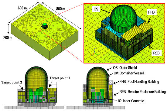
Figure 5.
Outline of the model of the nuclear power plant (NPP) buildings.

Table 1.
Example of the property of the concrete material on seismic walls.
Table 2.
Computation Scale.
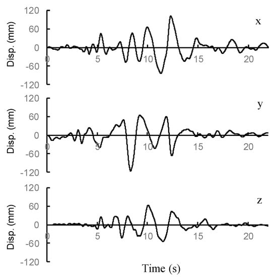
Figure 6.
Input seismic motion of displacement posed to the bottom of the soil domain.
In order to save the degrees of freedom, the authors employed a hybrid model of solid elements and structural elements. Figure 7 illustrates the part to which the structural elements are applied. Shell elements and beam elements are shown as green and red, respectively. The structures with structural elements are rigid or elastic without complex seismic response. The solid elements were applied to the reinforced concrete walls which were against a seismic load which had a possibility to experience a large deformation. Moreover, the model took advantage of multi-point constraints (MPC) at the part of the connection without any damage. As a result, the degrees of freedom were suppressed to 1.5 million.
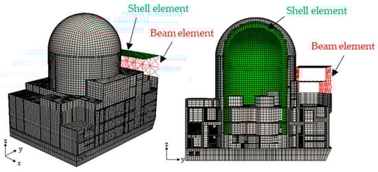
Figure 7.
Application of hybrid model.
The computational performance was mainly examined. The elapsed time of this analysis was approximately 10 h, when we used a parallel computer of 64 cores. Though the computation of 64 cores is not significantly large, this elapsed time is short enough for practical use. This result shows the possibility of evaluating the seismic response of a whole soil-structure system using a high-fidelity model. Figure 8 shows the scalability of the computation, which is one of the most important performances of the HPC program. For this analysis, a shorter seismic input wave, which is extracted from the input seismic wave as 2.5 s duration including its principal shock, was applied. This result shows the scalability of elapsed time and the computation time of the solver is high. Moreover, the result also shows that the computation time of the solver occupied the majority of the elapsed time, which means that the development of the program presupposing the usage of the HPC solver works well.
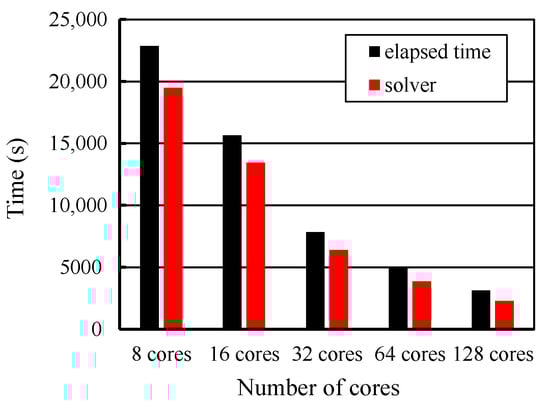
Figure 8.
Scalability of the computation; relation between the elapsed time and the number of cores used in each computation.
The work briefly showed the results of the seismic response analysis. Figure 9 presents the examples of the deformation of the NPP building and the distribution of stress. Shown is at the time of the step at which the maximum shear deformation took place during the analysis. These results indicate that a numerical analysis of a high fidelity model, which is enabled by using the HPC-FEM program, visualizes the local deformation and the inertial force which are caused by the seismic load with high spatial resolution.
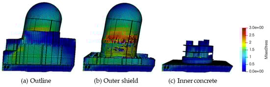
Figure 9.
Deformation and the distribution of stress.
Figure 10 exhibits the acceleration response and the acceleration response spectrum. These were measured for the two target points at the top level of the reactor enclosure building; each point is at the opposite side of the outer shield shown in Figure 5. The response and spectrum are quite different even though they are on the same level and such difference cannot be computed by using a simplified model, that is, an ordinary lumped mass model, in which responses at the same level are identical. It confirms a need for the analysis of a high-fidelity model for accurate estimation of local seismic responses which are used as input for equipment and facilities located in the NPP building. The results of the linear analysis are shown in this figure for the comparison with the non-linear analysis. The acceleration response spectrum is quite different in a certain range of frequency, which confirms the need for the non-linear analysis. Precise treatment of material non-linearity is needed to make the device design more rational. It should also be noted that such high-fidelity model with the precise treatment of material non-linearity improves the inertial effect of SSI.
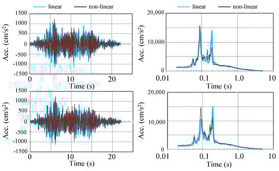
Figure 10.
Acceleration time-histories and response spectra at two target points, with linear and non-linear analysis.
5. Concluding Remarks
The study of SSI is diverse and involves several research areas such as engineering seismology, soil mechanics, foundation engineering, structural engineering and so forth. The numerical analysis can integrate the achievement of all the research areas. It should be supported by the fundamental physical theory shared by the research areas and advanced computer and computational sciences. This is the reason that the present review paper employs the continuum mechanics theory and the use of HPC. It is clarified that there is a wide range of numerical analyses of SSI ranging from a conventional analysis of a simplified model to the use of HPC for a high-fidelity model. All the numerical analysis must solve a mathematical problem that is consistent with an original Lagrangian problem of a soil-structure system according to the continuum mechanics theory. Then, we can choose a suitable numerical analysis depending on the level of the accuracy and resolution of a required solution.
As is seen in the literature survey, even though the 3D solid element based FEM analysis is becoming increasingly possible for ordinary civil engineering problems, yet the conventional simplified models are still being used even for the analysis of important structures such as nuclear power plants. These models developed in the era of lesser computational resources have been helping the engineering community since long. However, there is a need for their improvement by increasing the spatial resolution and the use of high fidelity models will be an important issue of future research to meet this need.
The use of HPC for the numerical analysis of SSI started recently and we will keep using computers of increasing performances. There are many issues that could be solved with the use of HPC; for example, we have to consider various types of constitutive relations for soil and structural materials, the effects of spread or pile footing, embedded or surface foundation, slip and detaching at the interface and the effects of uncertainty in actual soil and structure properties. It is necessary to develop the automated construction of a high fidelity model from CAD data. Keeping the diversity of related fields in mind, we consider that this study will be a first step to the advancement of the SSI study using HPC and hence we focus on the clarification of the SSI problem based on the continuum mechanics theory.
Author Contributions
Conceptualization, M.R.R. and M.H.; methodology, M.R.R.; software, H.M.; validation, M.R.R., H.M. and M.H.; formal analysis, M.R.R.; resources, M.R.R.; writing—original draft preparation, M.R.R., H.M.; writing—review and editing, M.R.R., H.M.; visualization, H.M.; supervision, M.H.; project administration, M.H. All authors have read and agreed to the published version of the manuscript.
Funding
This research received no external funding.
Conflicts of Interest
The authors declare no conflict of interest.
Appendix A. Rigid Body Interface between Structure and Ground
It is of interest to derive a governing equation for the movement of a rigid-body interface between a structure and ground since elaborated mathematical treatment is needed for the rigid body movement. We use the same Lagrangian, given by Equation (1) and consider the following general displacement function:
Here, for simplicity, we consider one-direction input and denote the displacement functions in and by and , respectively; rigid-body rotation is neglected even though it is straightforward to include it in a manner similar to rigid-body translation. A key issue is the continuity of displacement across the interface, , which is assumed to be rigid body. Setting on , we have rigid body given by for in . Thus, we must have on . This condition is implemented into by addition of this condition as a constraint, that is,
where is a Lagrange multiplier. A set of coupled differential equations are derived from for , and . Since plays a role of the traction acting on , both and are formally obtained for a given by solving the differential equation. Then, becomes an integral differential equation for , the form of which is very complicated.
Appendix B. Computation of Equation (17)
In deriving Equation (17) from the substitution of Equation (16) into Equation (1), we drop a few terms, assuming the symmetry of and . For instance, or is used, based on the assumption that or ( or ) is symmetric or anti-symmetric with respect to a horizontal coordinate, respectively. These integrations represent coupling effects of the displacement functions induced by rigid body translation and rigid body rotation, which vanish if certain symmetry holds for the functions; when is symmetric in the horizontal direction, the displacement function due to the rigid body translation and rotation ought to be symmetric and anti-symmetric, respectively. Therefore, some integrations taken over and are dropped in Equation (17).
References
- Kausel, E. Early history of soil-structure interaction. Soil Dyn. Earthq. Eng. 2010, 30, 822–832. [Google Scholar] [CrossRef]
- Roesset, J. Soil structure interaction, the early stages. J. Appl. Sci. Eng. 2013, 16, 1–8. [Google Scholar]
- Gulkan, P.; Clough, R.W. Developments in Dynamic Soil-Structure Interaction. In Proceedings of the NATO Advanced Study Institute on Developments in Dynamic Soil-Structure Interaction, Kemer, Antalya, Turkey, 8–16 July 1992. [Google Scholar]
- Lou, M.; Wang, H.; Chen, X.; Zhai, Y. Structure–soil–structure interaction: Literature review. Soil Dyn. Earthq. Eng. 2011, 31, 1724–1731. [Google Scholar] [CrossRef]
- Wolf, J.P. Dynamic Soil-Structure Interaction; Prentice-Hall: Englewood Cliffs, NJ, USA, 1985. [Google Scholar]
- Mylonakis, G.; Gazetas, G. Seismic soil-structure interaction: Beneficial or detrimental? J. Earthq. Eng. 2000, 4, 277–301. [Google Scholar] [CrossRef]
- Sezawa, K.; Kanai, K. Decay in the seismic vibration of a simple or tall structure by dissipation of their energy into the ground. Bull. Earthq. Res. Inst. Jpn. 1935, 13, 681–696. [Google Scholar]
- Sezawa, K.; Kanai, K. Energy dissipation in seismic vibration of actual buildings. Bull. Earthq. Res. Inst. Jpn. 1935, 13, 925–941. [Google Scholar]
- Reissner, E. Stationäre, axialsymmetrische, durch eine schüttelnde Masse erregte Schwingung eines homogenen elastischen Halbraum. Ing. Arch. 1936, 7, 381–396. (In German) [Google Scholar] [CrossRef]
- Massimino, M.R.; Abate, G.; Grasso, S.; Pitilakis, D. Some aspects of DSSI in the dynamic response of fully-coupled soil-structure systems. Riv. Ital. Geotec. 2019, 1, 44–70. [Google Scholar]
- Gazetas, G. 4th Ishihara lecture: Soil-foundation-structure systems beyond conventional seismic failure thresholds. Soil Dyn. Earthq. Eng. 2015, 68, 23–39. [Google Scholar] [CrossRef]
- Anastasopoulos, I.; Gelagoti, F.; Spyridaki, A.; Sideri, J.; Gazetas, G. Seismic rocking isolation of an asymmetric frame on spread footings. J. Geotech. Geoenviron. Eng. 2014, 140, 133–151. [Google Scholar] [CrossRef]
- Pecker, A.; Paolucci, R.; Chatzigogos, C.; Correia, A.A.; Figini, R. The role of non-linear dynamic soil-foundation interaction on the seismic response of structures. Bull. Earthq. Eng. 2014, 12, 1157–1176. [Google Scholar] [CrossRef]
- Anastasopoulos, I.; Gazetas, G.; Loli, M.; Apostolou, M.; Gerolymos, N. Soil failure can be used for seismic protection of structures. Bull. Earthq. Eng. 2010, 8, 309–326. [Google Scholar] [CrossRef]
- Gavras, A.G.; Kutter, B.L.; Hakhamaneshi, M.; Gajan, S.; Tsatsis, A.; Sharma, K.; Kohno, T.; Deng, L.; Anastasopoulos, I.; Gazetas, G. Database of rocking shallow foundation performance: Dynamic shaking. Earthq. Spectra 2020, 36, 960–982. [Google Scholar] [CrossRef]
- Drosos, V.; Georgarakos, T.; Loli, M.; Zarzouras, O.; Gazetas, G. Soil-foundation-structure interaction with mobilization of bearing capacity: Experimental study on sand. J. Geotech. Geoenviron. Eng. 2012, 138, 1369–1386. [Google Scholar] [CrossRef]
- Abate, G.; Gatto, M.; Massimino, M.R.; Pitilakis, D. Large scale soil-foundation-structure model in Greece: Dynamic tests vs FEM simulation. COMPDYN 2017. In Proceedings of the 6th International Conference on Computational Methods in Structural Dynamics and Earthquake Engineering, Rhodes Island, Greece, 15–17 June 2017. [Google Scholar]
- Massimino, M.R.; Biondi, G. Some experimetnal evidences on dynamic soil-structure interaction. In Proceedings of the COMPDYN 2015, 5th ECCOMAS Thematic Conference on Computational Methods in Structural Dynamics and Earthquake Engineering, Athens, Greece, 21–23 June 2015. [Google Scholar]
- Lysmer, J.; Kuhlemeyer, R.L. Finite dynamic model for infinite media. J. Eng. Mech. ASCE 1969, 95, 759–877. [Google Scholar]
- Lysmer, J.; Wass, G. Shear waves in plane infinite structures. J. Eng. Mech. ASCE 1972, 98, 85–105. [Google Scholar]
- White, W.; Valliappan, S.; Lee, I.K. Unified boundary for finite dynamic models. J. Eng. Mech. ASCE 1977, 103, 949–964. [Google Scholar]
- Liao, Z.P.; Wong, H.L. A transmitting boundary for the numerical simulation of elastic wave propagation. Soil Dyn. Earthq. Eng. 1984, 3, 174–183. [Google Scholar] [CrossRef]
- Zienkiewicz, O.C.; Bielak, J.; Shen, F.Q. Earthquake input definition and the transmitting boundary condition. In Advances in Computational Non-Linear Mechanics; Springer: Vienna, Austria, 1988; pp. 109–138. [Google Scholar]
- Deeks, A.J.; Randolph, M.F. Axisymmetric Time-domain Transmitting Boundaries. J. Eng. Mech. ASCE 1994, 120, 25–42. [Google Scholar] [CrossRef]
- Lee, J.H. Non-linear soil-structure interaction analysis in poroelastic soil using mid-point integrated finite elements and perfectly matched discrete layers. Soil Dyn. Earthq. Eng. 2018, 108, 160–176. [Google Scholar] [CrossRef]
- Coleman, J.L.; Bolisetti, C.; Whittaker, A.S. Time-domain soil-structure interaction analysis of nuclear facilities. Nucl. Eng. Des. 2016, 298, 264–270. [Google Scholar] [CrossRef]
- Solberg, J.; Hossain, Q. Non-linear time-domain soil-structure interaction analysis of embedded reactor structures subjected to earthquake loads. Nucl. Eng. Des. 2016, 304, 100–124. [Google Scholar] [CrossRef]
- Abell, J.A.; Orbovic, N.; McCallen, D.B.; Jeremic, B. Earthquake soil-structure interaction of nuclear power plants, differences in response to 3-D, 3 × 1-D, and 1-D excitations. Earthq. Eng. Struct. Dyn. 2018, 47, 1478–1495. [Google Scholar] [CrossRef]
- Yoshimura, S.; Hori, M.; Ohsaki, M. High Performance Computing for Structural Mechanics and Earthquake/Tsunamic Engineering; Springer International Publishing: New York, NY, USA, 2016. [Google Scholar]
- Quinay, P.E.B.; Ichimura, T.; Hori, M.; Wijerathne, M.L.L.; Nishida, A. Seismic structural response analysis considering fault-structure system: Application to nuclear power plant structures. Prog. Nucl. Sci. Technol. 2011, 2, 516–523. [Google Scholar] [CrossRef]
- Miyamura, T.; Tanaka, S.; Hori, M. Large-Scale Seismic Response Analysis of a Super-High-Rise-Building Fully Considering the Soil–Structure Interaction Using a High-Fidelity 3D Solid Element Model. J. Earthq. Tsunami 2016, 10, 1–21. [Google Scholar] [CrossRef]
- Veletsos, A.S.; Wei, Y.T. Lateral and rocking vibration of footings. J. Solid Mech. Found. Div. ASCE 1971, 97, 1227–1248. [Google Scholar]
- Luco, J.E. Impedance functions for a rigid foundation on a layered medium. Nucl. Eng. Des. 1974, 31, 204–217. [Google Scholar] [CrossRef]
- Kausel, E.; Roesset, J.M. Dynamic stiffness of circular foundations. J. Eng. Mech. ASCE 1975, 101, 771–785. [Google Scholar]
- Luco, J.E. Vibration of a rigid disk on a layered viscoelastic medium. Nucl. Eng. Des. 1976, 36, 325–340. [Google Scholar] [CrossRef]
- Gazetas, G.; Anastasopoulos, I.; Adamidis, O.; Kontoroupi, T. Nonlinear rocking stiffness of foundations. Soil Dyn. Earthq. Eng. 2013, 47, 83–91. [Google Scholar] [CrossRef]
- Gazetas, G. Formulas and Charts for impedances of surface and embedded foundations. J. Geotech. Eng. ASCE 1991, 117, 1–9. [Google Scholar] [CrossRef]
- Kubo, T.; Yamamoto, T.; Sato, K.; Jimbo, M.; Imaoka, T.; Umeki, Y. A Seismic Design of Nuclear Reactor Building Structures Applying Seismic Isolation System in a High Seismicity Region—A Feasibility Case Study in Japan. Nucl. Eng. Technol. 2014, 46, 581–594. [Google Scholar] [CrossRef]
- Okada, Y.; Ogawa, Y.; Hiroshima, M.; Iwate, T. Application of sway-rocking model to retrofit design of bridges. In Proceedings of the 14th World Conference on Earthquake Engineering, Bejing, China, 12–17 October 2008. [Google Scholar]
- Mylonakis, G.; Nikolaou, S.; Gazetas, G. Footings under seismic loading: Analysis and design issues with emphasis on bridge foundations. Soil Dyn. Earthq. Eng. 2006, 26, 824–853. [Google Scholar] [CrossRef]
- Ni, P.; Petrini, L.; Paolucci, R. Direct displacement-based assessment with nonlinear soil-structure interaction for multi-span reinforced concrete bridges. Struct. Infrastruct. Eng. 2014, 10, 1211–1227. [Google Scholar] [CrossRef]
- Yang, L.; Marshall, A.M.; Hajirasouliha, I. A simplified Nonlinear Sway-Rocking model for evaluation of seismic response of structures on shallow foundations. Soil Dyn. Earthq. Eng. 2016, 81, 14–26. [Google Scholar]
- Wong, H.L.; Luco, J.E. Soil-Structure Interaction: A Llinear Continuum Mechanics Approach (CLASSI); Department of Civil Engineering, University of Southern California: Los Angeles, CA, USA, 1980; CE 79–03. [Google Scholar]
- Lysmer, J.; Udaka, T.; Tsai, C.F.; Seed, H.B. FLUSH-A Computer Program for Approximate 3D Analysis of Soil-Structure Interaction Problems; Earthquake Engineering Research Center, University of California: Berkeley, CA, USA, 1975; Report No. EERC 75–30. [Google Scholar]
- Tabatabaie, M. SASSI FE Program for Seismic Response Analysis of Nuclear Containment Structures. In Proceedings of the International Workshop on Infrastructure Systems for Nuclear Energy, Taipei, Taiwan, 15–17 December 2008. [Google Scholar]
- Lesgidis, N.; Kwon, O.S.; Sextos, A. A time-domain seismic SSI analysis method for inelastic bridge structures through the use of a frequency-dependent lumped parameter model. Earthq. Eng. Struct. Dyn. 2015, 44, 2137–2156. [Google Scholar] [CrossRef]
- Carbonari, S.; Morici, M.; Dezi, F.; Leoni, G. A lumped parameter model for time-domain inertial soil-structure interaction analysis of structures on pile foundations. Earthq. Eng. Struct. Dyn. 2018, 47, 2147–2171. [Google Scholar] [CrossRef]
- Bucinskas, P.; Andersen, L.V. Dynamic response of vehicle–bridge–soil system using lumped-parameter models for structure–soil interaction. Comput. Struct. 2020, 238, 6270. [Google Scholar] [CrossRef]
- Maslenikov, O.R.; Chen, J.C. Uncertainty in Soil-Structure Interaction Analysis Arising from Differences in Analytical Techniques; U.S. Nuclear Regulatory Commission: Washington, DC, USA, 1982.
- Nova, R.; Montrasio, L. Settlements of shallow foundations on sand. Geotechnique 1999, 41, 243–256. [Google Scholar] [CrossRef]
- Chatzigogos, C.T.; Figini, R.; Pecker, A.; Salençon, J. A macroelement formulation for shallow foundations on cohesive and frictional soils. Int. J. Numer. Anal. Methods Geomech. 2011, 35, 902–931. [Google Scholar] [CrossRef]
- Figini, R.; Paolucci, R.; Chatzigogos, C.T. A macro-element model for non-linear soil–shallow foundation–structure interaction under seismic loads: Theoretical development and experimental validation on large scale tests. Earthq. Eng. Struct. Dyn. 2012, 41, 475–493. [Google Scholar] [CrossRef]
- Cavalieri, F.; Correia, A.A.; Crowley, H.; Pinho, R. Dynamic soil-structure interaction models for fragility characterisation of buildings with shallow foundations. Soil Dyn. Earthq. Eng. 2020, 132, 6004. [Google Scholar] [CrossRef]
- Chatzigogos, C.T.; Pecker, A.; Salençon, J. Macroelement modeling of shallow foundations. Soil Dyn. Earthq. Eng. 2009, 29, 765–781. [Google Scholar] [CrossRef]
- Cremer, C.; Pecker, A.; Davenne, L. Cyclic macro-element for soil-structure interaction: Material and geometrical non-linearities. Int. J. Numer. Anal. Methods Geomech. 2001, 25, 1257–1284. [Google Scholar] [CrossRef]
- Nakamura, N.; Akita, S.; Suzuki, T.; Koba, M.; Nakamura, S.; Nakano, T. Study of Ultimate Seismic Response and Fragility Evaluation of Nuclear Power Building Using Nonlinear Three-dimensional Finite Element Model. Nucl. Eng. Des. 2010, 240, 166–180. [Google Scholar] [CrossRef]
- Hori, M.; Maggededaera, L.; Ichimura, T.; Tanaka, S. Meta-Modeling for Constructing Model Consistent with Continuum Mechanics. J. Struct. Mech. Earthq. Eng. 2014, 9, 269–275. [Google Scholar] [CrossRef]
- Roh, H.; Lee, H.; Lee, J.S. New lumped-mass-stick model based on modal characteristics of structures: Development and application to a nuclear containment building. Earthq. Eng. Eng. Vib. 2013, 12, 307–317. [Google Scholar] [CrossRef]
- Jayasinghe, J.A.S.C.; Hori, M.; Riaz, M.R.; Wijerathne, M.L.L.; Ichimura, T. Meta-Modeling Based Consistent Mass Spring Model for Seismic Response Analysis of Bridge Structure. J. JSCE Appl. Mech. 2015, 71, 137–148. [Google Scholar] [CrossRef]
- Maekawa, K.; Okamura, H.; Pimanmas, A. Non-linear Mechanics of Reinforced Concrete; Taylor & Francis: Abingdon-on-Thames, UK, 2003. [Google Scholar]
- Yamashita, T.; Hori, M.; Oguni, K.; Okazawa, S.; Maki, T.; Takahashi, Y. Reformulation of non-linear constitutive relations of concrete for large-scale finite element method analysis. J. JSCE 2011, 67, 145–154. (In Japanese) [Google Scholar] [CrossRef]
- Motoyama, H.; Hori, M. Development and efficiency investigation of parallel computing seismic response analysis for high-fidelity model of large-scale reinforced concrete structures. In Proceedings of the SMiRT 25—The 25th International Conference on Structural Mechanics in Reactor Technology, Charlotte, NC, USA, 4–9 August 2019. [Google Scholar]


Publisher’s Note: MDPI stays neutral with regard to jurisdictional claims in published maps and institutional affiliations. |
© 2021 by the authors. Licensee MDPI, Basel, Switzerland. This article is an open access article distributed under the terms and conditions of the Creative Commons Attribution (CC BY) license (http://creativecommons.org/licenses/by/4.0/).