1. Introduction
The assessment of susceptibility and hazard are the most challenging issues in the field of rockfall risk estimation [
1]. In particular, the study of the hazard level requires three main steps [
2]: (i) the spatial identification of the involved areas; (ii) the computation of the rockfall intensity (measurable via the estimation of the kinetic energy of the falling blocks); (iii) the definition of the temporal occurrence of the phenomenon.
Referring to the first two items, several methodologies allow to identify the spatial evolution of the rockfall phenomenon. First, rigorous 3D analytical models permit to take into account the inertia of the rock block, achieving a reliable knowledge of the involved energy. More simplified models reduce the volume of the block to a dimensionless point (neglecting the effect of block shape and size) within a 2D or 3D framework. These models are generally used on large scales (i.e., site-specific) and local scales, following the recommendations of Corominas et al. (2014) [
3] for detailed risk analyses or to design protection works. Even more simplified models are used on small scales for territorial planning and preliminary study purposes [
2,
3,
4]. Necessarily, in these cases, the runout model should be both simple and reliable in order to overcome the limited availability of data and their epistemic uncertainties. Among a large set of methodologies, one of the most used is the Energy Angle Method (EAM), which was theorized by Onofri and Candian (1979) [
5] on the basis of the previous Fahrböscung approach, firstly proposed by Heim (1932) [
6]. The EAM is a simple frictional model in which the entire rockfall process is thought of as an equivalent sliding motion of a rigid block along a straight line (i.e., the “energy line”) connecting the rockfall source with the farthest outlying block at the foot of the slope. The inclination of the energy line is usually defined by the “energy angle” [
5,
7], called the “shadow angle” [
8,
9,
10] when the source point is located at the apex of the talus slope. Besides rockfall, the model is widely adopted even in the case of other slope instability phenomena, such as snow avalanches [
7,
11,
12,
13] and shallow landslides [
14,
15].
During the last decades, the EAM was implemented in several computer programs, even in the framework of GIS environment. First, Jaboyedoff and Labiouse (2011) [
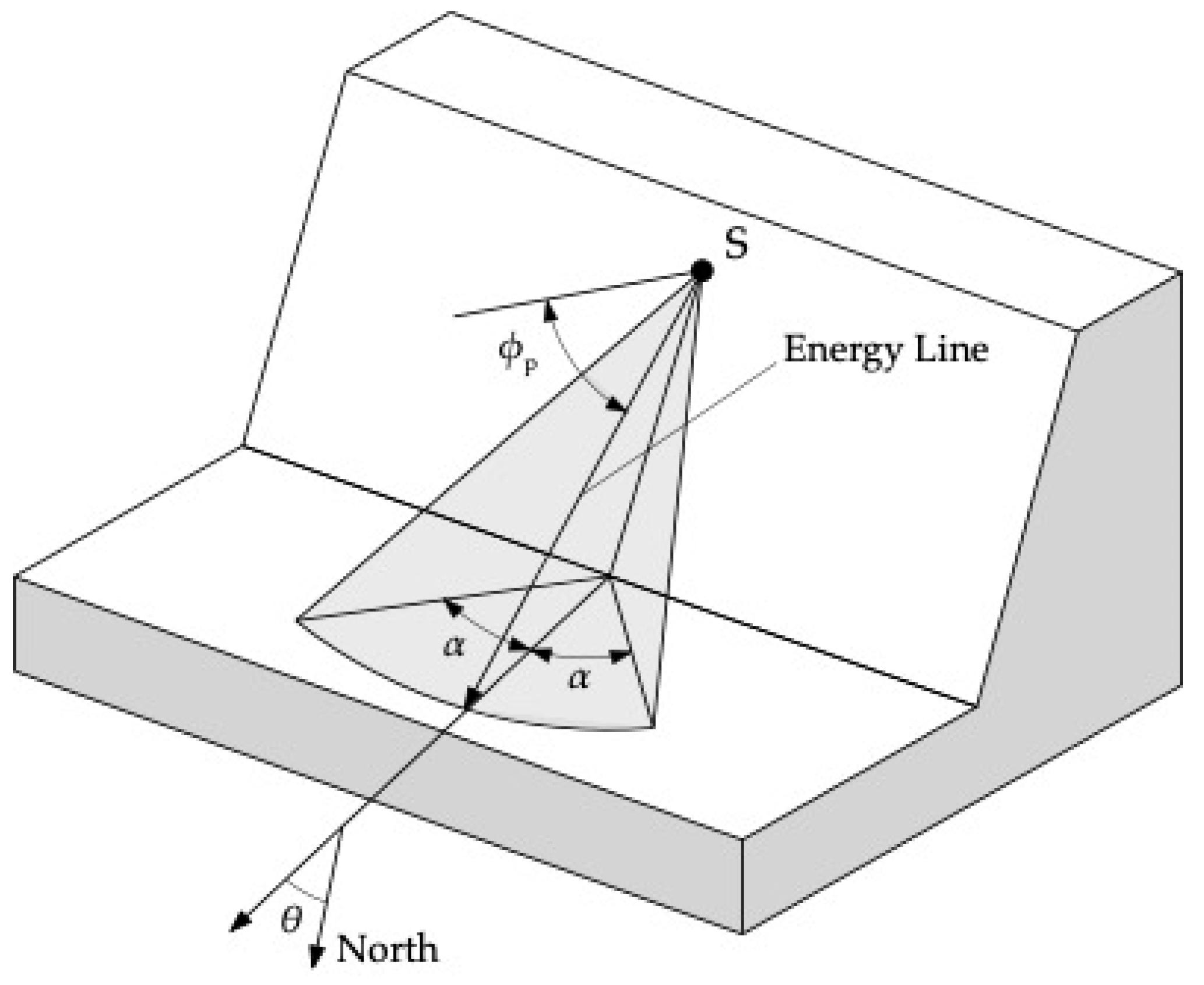
16] developed the CONEFALL tool, which is able to estimate the potential rockfall area only starting from a DTM and a grid file of the rockfall sources. In order to detect whether the DTM cell is located below the energy line (i.e., the topographical point is within the propagation area), CONEFALL introduces a series of cones having their apexes in the rockfall source points. The intersection of these cones with the surface of the slope gives the propagation area (
Figure 1). Then, a simple energy balance provides the kinetic energy within the computed area. This 3D variation of the EAM is usually addressed as Cone Method (CM). The CM was further implemented in QPROTO [
17], a cross-platform open-source plugin developed for the QGIS 3 environment. Starting from some rockfall source points, the tool performs a viewshed analysis via the application of the GRASS GIS function
r.viewshed [
18]. Such an analysis is limited to a visibility cone, described in space by three angles: (i) the dip direction
θ, which defines the orientation of the cone with respect to the north; (ii) the energy angle
, which defines the cone in the vertical plane; (iii) the lateral spreading angle
, which encloses the cone in the horizontal plane.
At this point, a reasonable question might arise about the values to be used to characterize these angles (hereafter “cone angles”) within preliminary hazard analyses. Many authors have suggested a statistical solution to estimate
as a function of the percentage of the stopping points [
16,
19]. For instance, Onofri and Candian (1979) [
5], on the basis of on-site observations, noted that the 100% of the observed blocks stopped for
> 28.5°, while the 50% for
> 32°. Otherwise, a statistical analysis of the Principality of Andorra case study returned the value 41.3°, 39.5° and 36.9° for the 90, 99 and 99.9 percentiles, respectively [
20,
21]. Lied (1977) [
8] found that all the blocks stopped with angles in a range between 28° and 30°. Other authors proposed a maximum value for the angles, by means of different case studies. Evans and Hungr (1993) [
10] set a maximum shadow angle of 27.5° and a
of 24°, while Wieczorek et al. (1998) [
9] suggested a lower value for
, equal to 22°. Such a wide variability and the strong site-dependence of these studies lead us to the conclusion that a reliable representation of rockfall phenomena through the energy line should take into account the influence of block characteristics (e.g., shape, volume, resistance) and slope conditions (e.g., inclination, length, roughness, vegetation). Some studies have been carried out in the last years to highlight the role of some of these factors on the energy line. For example, Rickli et al. (1994) [
22] introduced a classification of the angles taking into account the resistance and the size of the block by referring to German mountain real cases: (i)
= 33° for small rocks if the resistance is low and the underground smooth or the blocks are larger, resistance is high and the slope is rough; (ii)
= 35° for medium-sized blocks; and (iii)
= 37° for small blocks with high resistance and very rough slope. More recently, Volkwein et al. (2018) [
23] presented the first results of an extensive in situ rockfall testing aimed at gaining very detailed information on the trajectories of falling blocks on a grass slope, that can be very useful to calibrate both numerical trajectory simulations and simplified analyses based on the energy line. These examples demonstrate that, for a proper use of the Cone Method, the need exists to analyze the dependence of the energy line to all the factors that influence rockfall trajectories.
With regards to the lateral angle
, a few indications can be obtained from the literature. In general, the lateral dispersion of rockfall phenomena depends on three factors [
24]: macro-topographic (slope morphology, steepness, presence of channels, longitudinal and transversal ridges etc.), micro-topographic (roughness of the slope surface), and dynamic (interaction between block and slope, trees, protection works etc.) factors. Starting from numerical models, Azzoni et al. (1995) stated that lateral dispersion usually amounts to 20% of the slope length, decreasing for short and steep slopes, but can be much larger for irregular or channeled slopes [
25]. A higher value, equal to 34% of slope length, was found by Agliardi and Crosta (2003) [
26]. Crosta and Agliardi (2004), adopting an original rockfall 3D simulation program, carried out a series of analyses on simulated slopes with different steepness, roughness and pixel size [
24]. They found that lateral dispersion did not vary considerably with reference to slope steepness, with maximum values generally lower than 10%. Otherwise, the higher was the slope roughness, the larger was the lateral dispersion.
This wide variety of the results leads us to conclude that, except some very rough indication, at present, it is not possible to correlate the cone angles with the characteristics of the rockfall scenario under study through literature data, and more detailed analyses are needed. Thus, in this paper a new method to estimate the influence of slope and block features on the QPROTO input parameters (
and
) is proposed with the aim of providing the users of a set of reliable input parameters potentially tailored to different slope typologies. In particular, the role of the slope inclination, forest coverage, size and shape of the block are investigated. A series of trajectory analyses were carried out to this aim on artificially created slopes (called “synthetic slopes” hereafter) adopting the probabilistic process-based software Rockyfor3D [
27]. Finally, the findings are validated and exemplified with reference to some real case studies belonging to the north-western Italian Alps.
2. The QPROTO Plugin
The QPROTO plugin (QGIS Predictive ROckfall TOol) [
17] was created for implementing the Cone Method [
16] in the QGIS environment, a user-friendly open-source geographic software, created and supported by the Open Source Geospatial Foundation (OSGeo). The plugin is based on the GRASS GIS 7 module
r.viewshed [
18], which allows to evaluate the visibility of the neighboring zones starting from a given set of viewpoints. Each of these points is the apex of a visibility cone covering a certain portion of the slope. As described in
Section 1, the geometry of the cone is determined by three different angles: the dip direction
θ, the energy angle
and the lateral angle
(
Figure 1). A further visibility distance introduces the maximum distance to which the analysis can be extended. The basic assumption is the correspondence between the viewpoint and the source of rockfall event: the whole viewed zone of the slope can potentially be reached by the boulder paths starting from the considered source.
When diffused source points are considered, the plugin allows to define the rockfall subjected zones generated by the overlapping of the produced visibility cones. In this way, a frequency map can be obtained: the zones characterized by higher frequencies refer to more visible points, i.e., areas that can be easily reached by fallen blocks coming from different source points and that can be interpreted as the most prone to be affected by this type of phenomenon.
Through the Cone Method (
Figure 2), it is also possible to quantitatively evaluate the velocity
v(x,y) of the fallen block in each point
P(
x,
y) of the topographic surface by using the following relation (Equation (1)):
where
g is the gravity acceleration,
x0 and
y0 are the coordinates of the source point
S, H(x0,y0) the elevation of the source point,
hp(x,y) the elevation of the topographic surface at point
P(
x,
y) and
ϕp the energy angle. In
Figure 2, the heights defined at the location of point
P(
x,
y) are linked to the energy balance of the falling block.
H(x0,y0) represents the total energy content of the block which is defined by the energy conservation principle as the sum of potential
hp(x,y), kinetic
hk(x,y) and friction or dissipative contributions (
).
Thus, it is possible to obtain the kinetic energy
Ek(x,y) at each point of the cone adopting the following relationship (Equation (2)):
where
m is the mass of the block and
v(x,y) its velocity at the point
P(
x,
y).
It has to be considered that the calculated energy does not take into account the combination of free flight, bouncing, rolling and sliding phenomena that actually occur during the propagation phase: all these phenomena are simulated through an equivalent sliding motion along the above-mentioned plan with inclination equal to . Velocity and energy values obtained in this way need to be interpreted with great caution, especially by comparing them with the result of more accurate propagation analyses. Anyway, energy estimation through the Cone Method can lead to a preliminary estimation of the hazard, useful to highlight the most critical zones of a wide area in terms of process intensity as well as susceptibility.
To include the characteristics of the rockfall sources in the hazard estimation, the QPROTO plugin allows to assign a different propensity to detachment index (DI) to each source point. DI can be seen as a weight highlighting the most likely source zones to trigger rockfall events and can be defined as a function of the available information related to the study area (i.e., historical data, fracture density maps, inclination of the slope in the source zones) combined with the results of rapid on-site survey [
28,
29]. DI allows to calculate a weighted frequency map (i.e., a susceptibility map) and time-independent hazard maps (spatial hazard maps). The susceptibility map is a raster file describing how the rockfall phenomenon is distributed over the invasion area, highlighting the most affected zones through a very simplified and not temporal probability to be reached. The time-independent hazard maps combine the information about the detachment propensity of each source point with the estimated kinetic energy in a given cell of the invasion zone. Thus, each cell of these hazard maps corresponds with weighted energy values. It has to be noted that, with reference to the definition of the index DI, the hazard maps can be called as “time-independent” because of the difficulty in collecting information concerning rockfall temporal occurrence at a small and medium scale. However, in case a temporal probability of occurrence is available (e.g., an estimation of the return period), the QPROTO plugin allows to calculate a time based rockfall hazard map by substituting (or including) this information to the propensity to detachment index. However, these aspects of the hazard analysis are not relevant in this paper and thus we will not go more in detail. Further information on the hazard calculation can be found at
https://plugins.qgis.org/plugins/qproto/ (accessed on 17 January 2021) [
17].
For the proper execution of QPROTO, in addition to the QGIS algorithms, GRASS 7 and SAGA GIS open-source modules are required to create and manage vector and raster files and perform the viewshed analysis. A set of source points, each of them representing a single block, is created by the user within defined source areas. At each source point, the attributes listed in
Table 1 have to be associated. Some of them can be easily inferred from the analysis of the DTM, such as point elevation and aspect; others have to be estimated on the basis of the available information about the slope geometry and condition, such as the energy angle
, the lateral angle
and the detachment propensity DI. Finally, boulder mass can be related to a specific scenario, characterized by a reference block volume.
The main results of the QPROTO analysis are 10 raster files, listed in
Table 2. The first raster (count) refers, for each cell belonging to the runout area, to the unweighted passage frequency, i.e., the number of source points viewing the cell. The second raster (susceptibility) shows the weighted passage frequency (i.e., the sum of all the detachment index DI of the source points viewing the considered cell). The following three raster maps (v_min, v_mean and v_max) concern the minimum, mean and maximum velocity, respectively, evaluated in each cell by using Equation (1). Based on these last three rasters, the corresponding energy raster maps (e_min, e_mean and e_max) are obtained adopting Equation (2). Furthermore, the two time-independent hazard maps (w_en and w_tot_en) are provided by multiplying the detachment index DI and the kinetic energy in each cell of the runout area. In addition to these outputs, the Finalpoints vector shapefile and the _log.txt logfile containing the report of the analysis are generated separately.
After the computation, the outputs are automatically loaded within the QGIS environment. Velocity and energy rasters are expressed in (m/s) and (J), respectively. Although the susceptibility and hazard files are expressed in (J), a classification on a five-level scale (i.e., very low, low, medium, high and very high) is adopted.
3. Estimation of the QPROTO Input Parameters: The Proposed Methodology
The application of the Cone Method through the QPROTO plugin requires the definition of a small number of parameters (the cone angles) that represent the reference scenario in terms of slope condition (geometry, forest coverage, etc.) and block characteristics (shape, volume). Indeed, such characteristics strongly influence the rockfall runout [
30,
31], and, thus, any hazard assessment methodology, although simplified, has to take them into account to obtain reliable as well as conservative results. To relate the cone angles to both block and slope features, a fully computational methodology was developed, based on simplified parametric analyses, able to provide some indications to QPROTO users for estimating the most reliable input parameters. The main steps of the proposed method are the following:
Creation of simplified synthetic slopes and definition of their geometrical and physical characteristics;
Execution of a statistically representative number of detailed 3D rockfall numerical simulations on the synthetic slopes in different conditions (presence of forest, block volume and shape etc.), on the basis of the parametric variation of some variables;
Statistical interpretation of the results in terms of energy angle and lateral angle;
Correlation of the cone angles with the considered variables;
Interpolation of the results and definition of charts for the estimation of the cone angles;
Validation of the results through their application to real study cases.
Among the available 3D rockfall simulation software, the Rockyfor3D model was used [
27] for carrying out the parametric analyses because of its numerous advantages. In particular, it provides results in statistical terms and allows to consider the three-dimensional character of the falling block and the possibility of simulating impact with trees. This latter aspect assumes a crucial importance because of the dissipative capacity that trunks can offer and the protective role of forests against rockfall.
However, it is important to highlight that Rockyfor3D is not a fully three-dimensional model because it uses equivalent spherical shapes to compute block position, rebound on the slope surface and impacts against trees. In particular, the smallest sphere is adopted to calculate whether the block impacts a tree, while a larger one is used when block-soil interactions are involved. The shape changes operated by Rockyfor3D can influence the energy angles, especially in cases when the slenderness of the block cannot be neglected. Therefore, in this work, only isometric (cubic and spherical) shapes were taken into account, and the role of the slenderness was disregarded. This will be further investigated through different methods.
Because of the quick nature of the plugin QPROTO and the numerical basis of the methodology, many simplifying hypotheses were introduced in the analyses, which involved both slope and block characteristics. Of course, these hypotheses influence the applicability of the obtained results to real rockfall cases. In view of the foregoing, the present work assumes a double significance: first, the results of the analyses could be used within QPROTO or other small-scale methods to perform quantitative preliminary analyses of rockfall hazard. Second, the proposed method can be tailored to other types of slope and block features to include in the results any rockfall scenario not yet included. In the following sub-sections, a complete description of the methodology and the simplifying hypotheses is provided.
3.1. Synthetic Slopes
The first step of the proposed methodology consists of the creation of several synthetic slopes where the propagation analyses will be carried out. These slopes are numerically created with an automatic and specifically developed Matlab code. Following some examples from the literature [
24], in this work, the synthetic slopes are composed of three consecutive ramps (or zones), as can be seen in
Figure 3. Each zone has a specific role in the rockfall simulation and its own different inclinations, geometrical and physical properties. These properties have to reproduce some typical conditions (height, inclination, forest coverage, soil types, roughness etc.) of real mountain slopes subjected to rockfall phenomena. “Zone 1,” or the “detachment zone”, with a constant inclination
with respect to the horizontal plane, represents the rock face from which the falling block detaches. For the sake of simplicity, only a single point within this area can originate the rockfall phenomenon. This point is the same for all the analyses and is located at the elevation of 270 m. “Zone 2,” or the “transit zone,” represents the propagation zone in which the falling block gradually loses its potential energy. To simulate a range of real slopes as wide as possible, the inclination of zone 2 can assume three different values: 30°, 45°, and 60°. Within this zone, the possible variation in forest coverage was also considered, as it will be better described in the following. Finally, “Zone 3,” or the “stopping zone,” is composed by a pseudo-horizontal plane (
) in which the falling blocks stop after the complete dissipation of their kinetic energy. No variation of the difference in height between the source and the foot of the slope is considered: in all the analyses, it is constant at 270 m. Such a height can be representative of many real rockfall events, but uncertainty increases when the source is located at different heights. This aspect is of great importance in the trajectory path of rockfall, and further investigation are needed to include the elevation of the rockfall source among the variables influencing the QPROTO parameters.
Further information about the synthetic slopes is needed to properly perform the rockfall simulations. Therefore, some physical properties concerning the three above-mentioned zones were introduced. These properties were defined according to the specific requirements needed by Rockyfor3D. First, the “soil type” describes the elastic behavior of the soil coverage. For both zones 1 and 2, we adopted soil types “compact soil with large rock fragments” (i.e., soil 4), with normal restitution coefficient in the range (0.34, 0.42). For zone 3, we adopted the more plastic “fine soil material” (i.e., soil 1), able to faster dissipate the kinetic energy of the block. Normal restitution coefficient in the range (0.21, 0.25) are associated by Rockyfor3D to this soil type. The above-mentioned soil types can be considered as roughly representative of most of the slopes in the Alpine environment and were taken constant in all our analyses. Especially in zone 2, as elastic as possible soil properties were considered in order to take into account the worst energy dissipation condition during the block–slope interaction and to obtain precautionary results.
The presence of the forest was considered only in zone 2. In particular, a conifer forest was assumed because of the lower resistance of this type of trees [
32,
33,
34], with a diameter at breast height (DBH) of the trunk equal to 35 ± 1 cm, which corresponds to a medium resistance capacity. Of course, the results are to be referred to real slopes characterized by forests of similar characteristics. For generalizing these results, a sensitivity study of these parameters will be carried out in the future. With regards to forest density and with the aim of fixing upper and lower limits to the range of variation of the results, two cases were considered: absence of trees (0% forest density) and dense forest coverage (100% forest density). A forest density of 100% can be assumed as 1 tree per cell of the DTM [
35], which means 400 trees/ha if a 5 m DTM is used, as in this case.
A brief recap of the geometrical and physical characteristics of the synthetic slopes adopted in this work is provided in
Table 3. To carry out the trajectory analyses, all geometrical and physical characteristics of the synthetic slopes were saved within raster files with a cell size resolution of 5 m.
3.2. Parametric Analyses
On the basis of the synthetic slopes described in the previous
Section 3.1, several parametric analyses were performed by combining both slope and block features. Inclination and forest coverage density of zone 2 were varied among the values listed in
Table 3. With reference to the block characteristics, a density of about 2500 kg/m
3 was introduced and the following five classes of volume were assumed for the parametrical study: 0.1, 0.5, 1.0, 5.0 and 10.0 m
3. Finally, both spherical and cubic shapes were taken into account in the Rockyfor3D simulations. In
Table 4, a recap of the main characteristics of the blocks adopted in this work is reported. Finally, the probabilistic nature of Rockyfor 3D [
27] allowed to perform 20,000 launches for each analysis in order to acquire a statistically representative number of simulations, necessary for a reliable statistical interpretation of the results.
3.3. Statistical Interpretation of the Results
The outputs of the trajectory analyses provided by Rockyfor3D are many raster files showing the distribution on the slope of block velocity, energy, stopping points, etc. Here, the interest is focused on stopping points, whose position allows to estimate both the cone angles
and
. In
Figure 3, an example of the definition of
and
is shown, with reference to the rockfall source point S and the
i-th stopping point
. Thus, 20,000 values for both the angles can be computed as follows (Equation (3)):
where
and
are the coordinates of the rockfall source S and the i-th stopping point
respectively.
The goal of this paper is to produce a tool for the definition of a couple of values
representative of the analyzed scenario in terms of block and slope characteristics, to be associated to the rockfall source points by the QPROTO users. To reach this goal, a single representative value has to be selected among the 20,000 results obtained through Equation (3). Thus, starting from the population of
and
computed values, the cumulative distribution functions (CDFs, hereafter) were defined (
Figure 4a,b). Since representative angles should be conservative, i.e., should be related to the maximum possible extension of the invasion zone, the 2nd percentile (
) was selected as representative of the energy angle CDF. On the contrary, the 98th percentile (
) was adopted for the lateral angle CDF, in order to consider the maximum lateral dispersion of the trajectories. It is worth noting that these two angles are not related to each other. In other words, the trajectories that provide
angle are not the same ones that provide
. This can be easily observed if the cone angles are plotted into a bivariate plane. In
Figure 5a the three-dimensional histogram of the cone angles analyzed in
Figure 4 is reported: it can be seen that the majority of the results (high occurrence frequency) are related to lateral angles lower than 2° and energy angles around 25° (
Figure 5b). This is due to the simple geometry and the peculiar symmetry characterizing the synthetic slopes adopted in this work. To obtain more general results that can be used in real cases, more conservative percentile values need to be considered.
The result of this simple statistical data processing is a couple of values (
;
) associated to different slope and block characteristics, useful to highlight the influence of each characteristic and to estimate the parameters in susceptibility and hazard analysis with QPROTO. These findings will be presented and discussed in the following
Section 4.
5. Discussion
On the basis of the proposed methodology, some conservative values were provided for the energy angle
in the case of isometric blocks, as a function of slope inclination, forest coverage and block volume. Such values can be considered as conservative because they refer to the second percentile of the CDF: in 98% of cases, these angles could be exceeded and, consequently, blocks could run shorter paths along the slope. Therefore, the dataset can be easily adopted as a starting point for preliminary and quick analyses within the QPROTO environment, as will be shown in
Section 6.
To organize the findings of the parametric analyses and to extend their validity to values of the variables not directly included in the analyses, an interpolation of all the data was performed, resulting in the charts of
Figure 11. The kriging regression technique was adopted in order to obtain the best linear prediction of the intermediate values. The curves represented in
Figure 11 allow to estimate the energy angles for any slope inclination ranging between 30° and 60° referring to isometric shapes and block volume between 0.1 and 10 m
3 scenarios.
Figure 11a refers to slopes without trees while
Figure 11b is related to dense forest simulations. Intermediate forest density can be associated to interpolated values between the two sets of curves.
Here, it can be useful to summarize the main results of this work. In particular:
Computed energy angles can reproduce the mitigation effect of dense forests located on the transit zone of the slope;
The growth of a block volume causes the reduction of the energy angle and provide larger invasion areas;
The growth of slope angle causes the increase of the energy angle and the reduction of the invasion area.
On the basis of the above-described observations, our findings are consistent with several literature works, real case observations and experimental activities [
10,
30,
36,
37,
38,
39].
With reference to the lateral angle
, the 98th percentile of the CDF was considered as a reference value in order to maximize the lateral dispersion of the trajectories. Unfortunately, in many cases of our analyses, the lateral angles were affected by the presence of blocks stopped just below the rockfall source point. These deposited blocks were typically characterized by high values of the lateral angle, which are considerably larger than those obtained for the blocks that reached the foot of the slope. Such values strongly overestimate the maximum lateral spreading of blocks. To better understand this issue, it is possible to refer to the simulations performed with a spherical unitary block reported in
Figure 7a in the forested scenario, where blocks are distributed over the transit zone. Assuming
= 18.4° in the Cone Method, this can result in a considerable overestimation of the runout area, since the elongated shape of the stopping points can barely be represented by a cone, with the apex at the source point and the maximum width at the foot of the slope (
Figure 12). Thus, in this case, the statistical data do not seem to be adequate to reproduce the rockfall invasion zone and more reliable methods are necessary. In the following improvements of the research, some qualitative considerations will be adopted and tested with reference to some real case studies in order to get more realistic results.
6. Validation and Examples
The results achieved in this work were applied to two different study cases belonging to the Susa Valley, in the north-western Italian Alps. First, the results were validated with reference to the rockfall event that occurred in 2011 in the Cels-Morlière hamlet. A second validation was done for the rockfall event that occurred in 2010 in the Melezet hamlet. Finally, the results were applied to a larger portion of the slope to perform a forecasting rockfall analysis for the site of Melezet. The location of the two sites is reported in
Figure 13.
The Cels-Morlière hamlet (UTM: 4996137 337399 32T) is located in the municipality of Exilles, on the left hydrographical bank of the Dora Riparia river. The site has an elevation of 850 m a.s.l. and is overlooked by a largely fractured rock face, with its peak at 1400 m a.s.l. Cels-Morlière has historically been subjected to high-intensity rockfall events that often reached and damaged several buildings. The most recent event occurred in 2011, when a cluster of three blocks (each of them with a volume of about 5 m3) destroyed a flexible net barrier whose capacity is estimated around 800 kJ and hit three buildings. On average, the slope involved in this event is inclined of about 45°. A back-analysis of the event was first conducted by means of Rockyfor3D. A pre-event DTM with a resolution of 5 m was used, and 5 m3 blocks with a rock matrix density of about 2600 kg/m3 were simulated from the detachment niches, defined on the basis of event reports and the available digital cartography.
A broad-leaf forest with a density of 400 trees/ha was assumed to cover the slope, on the basis of qualitative observation of the orthophoto and the available forest inventories provided by the Piedmont Region. A flexible net barrier of 800 kJ capacity and 4.5 m height was also considered. The result of the back analysis is given in
Figure 14a in terms of mean kinetic energy. It is possible to observe that blocks keep descending beyond the existing protection works and arrive at the building’s location (Blds. 1 to 3) with the mean energy ranging between 500 kJ and 1500 kJ. These values seem slightly overestimated if compared to the observed damages (for Blds. 2 and 3, the estimated energies are in the range between 500 kJ and 1000 kJ), but they are acceptable, since the trajectory analysis has to be precautionary [
2].
To validate the proposed methodology for the estimation of the QPROTO parameters, a back-analysis of the 2011 event was conducted by means of QPROTO as well.
The main inputs of the QPROTO back analysis are the average slope inclination of 45°, a block volume of 5 m
3 and a dense forest coverage (400 trees/ha). The energy angle
= 34° can be extracted from
Figure 11b. A value of
= 10° was finally assumed to completely define the visibility cones. Seven points were selected inside the source area and the attributes listed in
Table 1 are associated to each of them. Finally, since it is a simulation of a real event, a constant propensity index DI = 1 was assumed. The result of the analysis is shown in
Figure 14b, again in terms of the mean kinetic energy. The comparison between
Figure 14a,b shows that QPROTO results are overestimated both in terms of invasion area and mean energy, involving a portion of the hamlet on the right side of the damaged buildings. It is worth noting that the analysis with Rockyfor3D considers the flexible net barrier of 800 kJ capacity, which played a role in the rockfall event, decelerating blocks and reducing their kinetic energy. However, this role seems weak, as shown in
Figure 14a, since the capacity of the barrier is low with respect to the kinetic energy of the blocks. At the current state of the work, it is not possible to consider how the presence of protective works on the slope can influence the energy line, and thus, its angle. Therefore, the preliminary QPROTO analysis does not consider this effect, and therefore, leads to a conservative result. On the basis of these observations, it is possible to conclude that the results obtained are acceptable and encouraging for future implementations.
The second study case is referred to the site of Melezet. The investigated area (UTM: 4994268 319183 32T) is located 2 km south-west of Bardonecchia at elevation around 1400 m a.s.l. It develops along the provincial road no. 216, connecting the Italian Susa Valley to the French Vallée de la Clarée. During the last four decades, the slope has been affected by intense and extremely damaging rockfall phenomena that involved both the Melezet hamlet and the provincial road. The last documented event dates back to May 2010, when a rock face approximately 30 m high and 25 m wide collapsed, involving a volume of about 2000 m
3. The fallen blocks partially hit and damaged the existing embankment located along the provincial road, and some boulders arrived on the provincial road, reaching the foot of the slope (
Figure 15). Such blocks damaged the provincial road, destroyed two isolated buildings and compromised the safety of inhabitants (
Figure 16b).
First, a back analysis of this event was performed, as an additional validation of the method. The adopted DTM with a resolution of 10 m is representative of the slope condition before the event. The back analysis was carried out by generating a set of rockfall source points within the collapsed portion of the rock face during the 2010 event. The attributes required by QPROTO were associated to each of the source points (
Table 5). The average inclination of the slope is equal to 35° and a dense forest coverage was assumed. Again, since it is a real event, a constant propensity index DI = 1 was considered. The reference block volume for the studied scenario is equal to 1 m
3, which was the average observed volume at the foot of the slope according to the event report prepared by ARPA Piemonte [
40].
On the basis of these data, the energy angle
= 34° can be extracted from
Figure 11b. Since the analysis on the lateral angle
seems to need some additional refinement, in this case, a parametric study was performed, looking for the value that best simulated the observed runout area: the best results were obtained assuming a lateral angle
The mean kinetic energy map resulting from the analysis is provided in
Figure 16a. The maximum values (about 1300 kJ) are reached at the mid-part of the slope, on the southern side of the runout zone, while lower ones (from few tens up to 700 kJ) are registered at the slope foot where the provincial road is located. In the zones where the two isolated buildings are located (Bld. 3), destroyed by a block impact on May 2010, the mean energy reaches 900 kJ, which is compatible with the observed damages (
Figure 16b). The presence of the embankment was not directly taken into account because of the limited effects that this protection work induced in the kinematics of the studied event.
Following this additional validation of the method, a new forecasting analysis on a more extended portion of land was carried out, to preliminarily analyze the slope in the neighbors and to estimate the susceptibility of the valley bottom.
The set of source points was obtained starting from 11 homogeneous areas (
Figure 17) established on the basis of reports produced by local technicians. The homogeneous areas were defined as portions of the rock face having uniform characteristics, such as slope orientation, elevation and structural characteristics. Within each homogeneous area, a set of source points was generated by referring to a DTM with resolution 5 m, representative of the condition of the slope after the event of May 2010. The points were randomly selected at the center of the 50% of the grid cells with an inclination larger than 45°. The result is a shapefile composed by 1687 points. Then, the attributes listed in
Table 5 were associated to each point. They were extracted either from the analysis of the DTM (elevation and aspect), or through the proposed method. A block volume of 1 m
3 and a block mass of 2600 kg were assumed as representative of the phenomenon with reference to all the homogeneous areas because not enough data were available to obtain a more detailed characterization. Since the aim of the analysis is to test the methodology for the estimation of the QPROTO parameters, the detachment propensity DI was set equal to 1 within each homogeneous area. This means that all the computed parameters have the same probability of occurrence within any point of the propagation area, and the maps “count” and “susceptibility” are equal. In other words, the susceptibility within the invasion zone only depends on the number of source points and on the cone parameters
and
For the definition of the energy angles, a simple study of the slope morphology below each homogeneous area was carried out, with particular reference to the average slope inclination. A dense forest coverage was finally assumed, according to the observation of some recent orthophotos. In
Table 6, the mean orientation of the slope and the corresponding energy angle
as resulting from the use of chart of
Figure 11b are listed for each homogeneous area. In
Figure 17, the distribution of the chosen energy angle values among the homogeneous areas is shown. Finally, on the basis of the results of the back analysis, a constant value of the lateral angle
= ± 12° was assumed.
The results obtained by the QPROTO analysis are shown in
Figure 18a in terms of the mean kinetic energy (kJ), and in
Figure 18b in terms of the susceptibility. In general, it is possible to observe that the local viability, modified after the May 2010 event, seems highly affected by the considered scenario of rockfall events. About 1 km of the new provincial road no. 216 was involved, as well as the local viability and two bridges over the Dora Riparia river. However, the two inhabited areas seem only marginally reached by the rockfall scenario. The most affected zone in terms of susceptibility (frequency) is located below areas 2 and 3, due to the orientation of the slope and the large extension of the homogeneous source areas (high number of source points). Additionally, the zones of the slope where the mean energy is higher are located below areas 2 and 3. Here, the mean energy values are around 1500 kJ just below the sources and around 800 kJ at the slope foot where the roads are located. This area was interested by the rockfall event of May 2010 and the results obtained here are consistent with those of the back analysis (
Figure 16a). The pre-existing embankment (
Figure 15) located below areas 2, 4, 6 and 7 cannot be considered in the QPROTO analysis. Thus, the results shown in
Figure 18 could be overestimated in that zone. The mean kinetic energy at the embankment location is estimated in the range between 500 kJ and 900 kJ, but more detailed analyses are needed to evaluate the efficiency of the embankment in stopping block trajectories.
It is worth noting that the difference in height between source points and the foot of the slope is not uniform among the homogeneous areas. In the case of areas 6, 8 and 9, such a difference is less than 100 m; areas 0, 1 and 4 are located at a height ranging between 100 and 200 m; areas 2 and 3 are at a height ranging between 200 and 300 m; areas 5, 10 and 11 (northern part of the site) are at a height ranging between 400 and 500 m. Since this aspect of slope geometry was not taken into account in the parametrical analyses, the results could be further refined in the future development of the research.
The proposed methodology allowed to estimate the parameters to be used in the susceptibility analysis in a very simple way, i.e., only on the basis of the DTM, the available cartography and some observation of the slope conditions. The results seem very encouraging for further development of the research, aimed at providing the QPROTO users with a reliable tool to calibrate their analyses to the site under study.
7. Conclusions
In this paper, a methodology for the quick estimation of the parameters needed to perform preliminary rockfall susceptibility and hazard analyses using the QPROTO plugin is presented. The plugin is based on the Cone Method and simplifies the complex path of a block along the slope with an equivalent pure sliding motion on a plane. The inclination of this plane with respect to the horizontal plane (i.e., the energy angle ) is the main parameter of the method, because it represents all the dissipative phenomena that occur during motion. The 3D implementation of the method includes the definition of a second angle that represents the lateral spreading of the phenomenon (i.e., the lateral angle ). Both the energy angle and lateral angle contribute to define a cone in the space. On the basis of this cone, QPROTO performs a viewshed analysis starting from some source points: all the zones of the slope that can be viewed by an observer located in the source point can be reached by a boulder detached from that point. To perform a susceptibility/hazard analysis with the QPROTO plugin, energy and lateral angles are the only equivalent parameters to be estimated, which should represent all the factors actually influencing the rockfall phenomena.
To provide QPROTO users with a tool able to calibrate the parameters that characterize the rockfall scenario under investigation, several parametric analyses deepening the influence of both slope and block features on the cone angles were performed. Each analysis consists of: (i) detailed rockfall simulations on synthetic simplified slopes and (ii) the statistical processing of the results to designate representative values of the angles. The main variables whose influence was parametrically evaluated are: slope inclination, forest coverage, block volume and shape. Other characteristics, such as elevation of the source point, length of the slope, soil type, roughness and slenderness of the block, were kept constant in this research and their effect will be further investigated in the future.
In the light of the findings of the parametric analyses, described in
Section 4, the following observations can be drawn:
For unitary blocks, a linear variation of both energy and lateral angles can be assumed as a function of slope inclination if non-forested slopes are considered and all the simulated blocks reach the stopping zone (i.e., the foot of the slope);
The effect of trees consists of reducing the extension of the runout area and, thus, in increasing the energy angle: a linear equation can be assumed as a function of the slope inclination in the case of . In the presence of trees, unitary blocks, in many cases, do not reach the foot of the slope and stop at the transit zone. Therefore, an overestimation of the lateral spreading can be observed as a consequence of the statistical processing of the data. Here, some preliminary results concerning the estimation of the lateral angle are reported, and more detailed analyses will be carried out in future works;
The influence of trees is also a function of the slope inclination: it is higher for less steep slopes and gradually decreases when the slope inclination increases. The linear variation of the energy angle with slope inclination is, therefore, less pronounced in the case of densely forested slopes;
Runout distance is strongly influenced by block volume: smaller volumes reach the closest distances on the slope, while larger blocks run farther. The variation of the energy angle with reference to block volume is not linear because it depends on the possibility that blocks reach the foot of the slope or stop in the transit zone;
Trees can influence the path of smaller blocks, reducing the extension of the runout area. This effect reduces when block volume increases;
Spherical and cubic blocks show similar behaviors. Considering the quick nature of the plugin QPROTO, a mean value of the energy angles can be considered as representative of generic isometric blocks.
The main output of the proposed methodology is a chart that interpolates all the obtained results and can be used to estimate the energy angle for different slope configurations and block volume scenarios. The chart was validated on the basis of some back analyses of real events that occurred in the Alpine environment. In this paper, the chart was finally used to provide the input variables required by the plugin QPROTO with reference to a preliminary susceptibility analysis carried out at medium and large scales. The example shows that the methodology, although very simplified, provides conservative and realistic results that are encouraging for further developments.
Several improvements arise from the work described here. With reference to the variables influencing the rockfall runout, the following items should be deepened:
The elevation of the source point with respect to the foot of the slope (and consequently the length of the transit zone) was kept constant in all the parametric analyses. Since it affects the length of boulder paths, it is supposed to strongly influence the results of the analyses and the cone angles. Further investigations on this topic will be carried out in the future in order to extend the parametric analyses to different elevation classes of the source points;
Block slenderness has not yet been taken into account because of the difficulty in interpreting the results provided by Rockyfor3D. This software is based on a hybrid model and simulates the block impacts (with the soil or with a tree) using equivalent spheres, whose dimensions are a function of the three initial dimensions of the block (height, width and thickness). This could affect the results in terms of runout area, and many uncertainties can be related to these changes of shape. To simulate the real behavior of blocks of elongated or slab shape, the use of a fully 3D rigid body model could be helpful and will be evaluated in the future;
The forest coverage adopted in this work, and described in
Section 3, has medium protective capacity against rockfall. To generalize the obtained results, in the future, a real sensitivity study will be carried out in order to consider different tree diameters, forest density, types of trees etc. Some interesting suggestions can be derived from previous studies on the protective role of forests, such as the one performed in the framework of the RockTheAlps project [
41];
In this work, a very smooth slope and elastic geomaterials were adopted in order to produce precautionary results. In case of small scales and preliminary rockfall analyses, very rough information concerning soil characteristics are usually available and using precautionary values could be the better solution;
The entire work is based on trajectographic analyses carried out on artificially created simplified slopes, to control the input variable with high levels of detail. The obtained results are in good agreement both with real cases and literature data but can be unrealistic if the slope is characterized by strong orientation gradient, which can deviate blocks from the original dip direction. Currently, the problem can be faced only through a high number of source points, in order to obtain a wider invasion area by the overlapping of differently oriented cones. A GIS study of slope morphometric features (concavity, convexity, curvature etc.) using well-documented real cases could help in introducing this aspect in the evaluation of the orientation and the lateral aperture of the cone. This will be investigated in the future development of the research. Moreover, some laboratory experiments carried out with scaled slopes could be useful to further validate the obtained results.
Finally, with reference to the QPROTO plugin, some improvements may concern the effect of protection works on the slope (e.g., flexible barriers). Currently, they cannot be taken into account in the viewshed analysis, causing an overestimation of the results. However, considering their protection role against rockfall events, it could be important to refine the results to overcome this unrealistic ovestimation. The influence of pre-existing protective works on rockfall runout is, however, the function of a number of factors, such as their geometry (length, height), their resistance, their position on the slope, their efficiency and their degree of conservation, which is mainly a function of time. A deep investigation of such factors seems to be still needed before extending the proposed methodology to consider their effects on the QPROTO parameters.


