Abstract
We analyze the auroral boundary corrected geomagnetic latitude provided by the Auroral Boundary Index (ABI) database to estimate long-term changes of core origin in the area enclosed by this boundary during 1983–2016. We design a four-step filtering process to minimize the solar contribution to the auroral boundary temporal variation for the northern and southern hemispheres. This process includes filtering geomagnetic and solar activity effects, removal of high-frequency signal, and additional removal of a ~20–30-year dominant solar periodicity. Comparison of our results with the secular change of auroral plus polar cap areas obtained using a simple model of the magnetosphere and a geomagnetic core field model reveals a decent agreement, with area increase/decrease in the southern/northern hemisphere respectively for both observations and model. This encouraging agreement provides observational evidence for the surprising recent decrease of the auroral zone area.
1. Introduction
Auroral oval regions, where charged particles accelerate along magnetic field lines from the magnetosphere down to the upper atmosphere [1,2], are of special interest to space weather due to the broad consequences of particle precipitation on technological systems. Solar events disturb terrestrial communications and geo-spatial positioning systems, cause satellite equipment degradation, and induce electric currents that may affect electric systems in highly populated areas [3,4,5,6,7,8]. Temporal changes in the auroral oval size modify the magnetosphere electric system; hence, there is a need to be prepared for the societal consequences of these variations as space weather might become more severe.
The auroral oval boundary is almost a circle whose center can be reasonably approximated by the eccentric geomagnetic dipole [9,10,11]. Hence, in such geomagnetic coordinates, the boundary latitude is nearly longitudinally invariant. Auroral boundaries depend directly on the Earth’s magnetosphere morphology, which depends on the geomagnetic field and solar wind conditions. The auroral oval size has an empirical correlation with the intensity of the simultaneous geomagnetic storm [12,13,14]. While the sun induces short-term variability, both core and solar origin magnetic forcings present additional long-term temporal changes, leading to secular variation of the auroral oval areas. This secular variation may lead to the secular variation of the auroral frequency at mid latitudes [15,16,17].
Since the advent of geomagnetic intensity measurements about 180 years ago (for a historical note, see [18]), the secular variation of the geomagnetic field is characterized by a rapid dipole moment decrease (e.g., [4,19,20,21]). Under the self-similarity hypothesis for a pure dipole magnetic field and a steady solar wind under quiet conditions, which is reasonable for a long-term average condition, polar cap boundary latitude, λp, scaling laws imply a variation in terms of the Earth’s dipole moment, M, according to cos(λp)∝(1/M)1/6 [22,23,24]. This means that for the present-day decreasing M, λp is expected to drift to lower latitudes with a consequent increase in the enclosed polar cap area for both hemispheres; moreover, since λp delineates the auroral oval inner boundary, area increase is also expected for the auroral oval. Indeed, the temporal changes of the polar cap and auroral oval areas are highly correlated [11,25].
However, Zossi et al. [11], using a model of the magnetosphere under steady interplanetary conditions and the IGRF-12 model [26] for the geomagnetic field, recently found that the secular variations of the northern polar cap and auroral oval areas disagree with these scaling laws, presenting a surprising decrease since 1940. In addition, even the increasing areas in the northern hemisphere prior to 1940 and in the southern hemisphere throughout the entire investigated period occurred at faster rates than those expected from the scaling law, indicating an impact of regional non-dipole geomagnetic field features on polar cap and auroral oval areas [11]. In an attempt to corroborate the modeled decreasing trend in the northern auroral oval area, and more generally to determine the observed rates in both hemispheres, we analyze here the auroral boundary corrected geomagnetic latitude provided by the Auroral Boundary Index (ABI) database [27,28,29], as an experimental measurement.
Solar and geomagnetic activities present long-term trends that may affect auroral ovals, including a longer time scale than the well-known quasi-decadal solar activity cycle [15,16,30]. Solar activity is the source of geomagnetic disturbances and gives rise to geomagnetic activity [31]. The latter results from the interaction between the solar activity (solar wind, heliospheric magnetic field) and the magnetosphere, producing several external current systems. In long-term periods, these two activities cannot be distinguished [32]. On decadal timescales, however, they might differ. Solar and geomagnetic activities lead to magnetic storms that may affect auroral ovals and many other magnetospheric features [33]. Classic indicators of solar activity are the sunspot number, Rz, and the 10.7 cm solar flux, F10.7; and those of geomagnetic activity are the indices termed Kp, Ap, aa, and Dst, which we define below. Both indices types differ on short timescales (less than 10 years) but resemble on increasing timescales, like the ~90-year Gleissberg cycle [34,35].
Since auroral ovals are strongly affected especially by geomagnetic activity [12,14], this effect should be filtered out to detect trends due to any other forcing. At the same time, a filtering process can generate ‘spurious’ trends, or variations, which might lead to erroneous conclusions [36]; since the long-term variation expected as a consequence of the geomagnetic core field secular variation is relatively small, these spurious effects might hinder the true variations. In this work, four successive filtering steps are applied to the auroral boundary data to minimize geomagnetic activity and solar activity effects and obtain its long-term variation, which originates from the geomagnetic core field secular variation.
2. Data Set and Auroral Area Calculation
In order to infer long-term variations in auroral oval boundaries and corresponding areas, we used the auroral boundary corrected geomagnetic latitude (from hereafter AB) provided by the Auroral Boundary Index (ABI) database [26,27,28], available for the period 1983–2016. To attribute these variations to a certain source, other sources of variations must be identified and filtered. In the case of auroral ovals, geomagnetic and solar activities that affect their variability are filtered. Remaining long-term variations are interpreted in terms of the geomagnetic core field secular variation. The data used is described below.
The AB, in units of degrees (°) is a derived quantity from measurements of the precipitating energetic particle spectrometer known as Special Sensor J (SSJ) carried by the Defense Meteorological Satellite Program (DMSP) spacecraft. As such, it is an estimate of the geomagnetic latitude position of the equatorward boundary of precipitating auroral electrons as determined by the SSJ/4 (F06 through F15) and SSJ/5 (F16 and beyond) (see details in [26,27,28,37,38]). Descriptions of the detector and the calibration of the instruments are given by Schumaker et al. [39].
AB data are available in yearly files at the CEDAR Madrigal Archive at http://cedar.openmadrigal.org, with a frequency of 2 to 4 data per hour. Each AB value has a quality control (QC) flag that is an integer from 1 to 3 (best = 1, good = 2, not good = 3). Each QC value characterizes about 1/3 of the total observed equatorward boundaries. There is also a “pseudo” Kp (pKp) estimate for each AB datum. Even though its numerical scale is almost continuous and with a different time spacing, considering QC = 1 and 2, pKp is highly similar to the usual Kp index whose scale is 0, 0+, 1−, 1, ..., with 8 values per day. The Kp index is a three-hourly planetary index derived from the standardized K index of 13 magnetic observatories located between 44° and 60° northern and southern geomagnetic latitudes. It is designed to measure solar particle radiation by its magnetic effects, and today it is considered a proxy for the energy input from the solar wind to the Earth. In addition to geomagnetic latitude, each yearly AB data file also provides the corresponding geomagnetic longitude and geographic coordinates (where for the latter, the z-axis is parallel to the Earth’s rotation axis and the x-axis points towards the intersection of the Equator and the Greenwich Meridian). Geomagnetic coordinates given in AB data files are corrected geomagnetic coordinates (CGM), which, by definition, are computed by tracing an IGRF magnetic field line through a specified point (latitude, longitude, altitude) to the dipole geomagnetic equator, then returning to the same altitude along the dipole field line and assigning the obtained dipole latitude and longitude as the CGM coordinates to the previously specified point [40]. As an example of the original data used in this work, the complete AB data series that is considering data with all QC and Kp values for 1990 are shown in Figure 1 in terms of geographic and geomagnetic corrected coordinates for the northern and southern hemispheres (which amount to 20,518 and 15,052 data points, for each hemisphere, respectively). Additionally, the data with QC = 1 and 2, and 0 < Kp < 2 (which amount to 5279 and 2832 data points, for each hemisphere, respectively), are also shown.
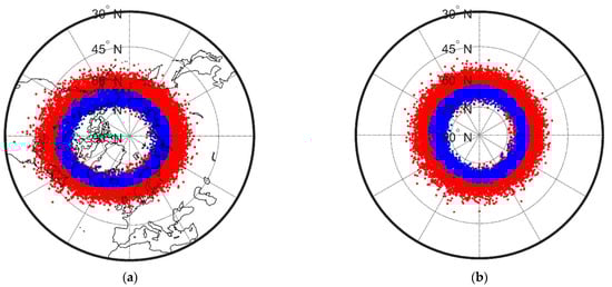
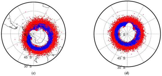
Figure 1.
Auroral boundary for the northern (a,b) and southern (c,d) hemispheres in geographic (a,c) and geomagnetic corrected coordinates (b,d) for 1990 considering the dataset with QC = 1 and 2 and 0 ≤ Kp ≤ 2 (blue dots); and QC = 1, 2, and 3 and all Kp values (blue + red dots).
The complete database we use, which results from concatenating the original yearly files from 1983 to 2016, has 1,676,550 AB data points. Figure 2 shows the number of data values per year, ranging between 16,460 and 75,210, with a mean of 49,310. The database contains a small number of erroneous measurements, pointed in the data list as negative pKp or pKp larger than 9, out of Kp scale, so we remove them. These points correspond to ~0.6% (9511) and 0.01% (114), respectively, of the data amount. Next, northern and southern hemisphere data were split into two series with 793,522 and 873,403 data points, respectively. Data with QC = 3 were also eliminated, leaving two time series of 471,740 and 651,933 data points each, containing northern and southern AB, respectively, with positive pKp values and QC = 1 and 2. In the southern hemisphere, there is a notch of missing data between −10° and 50° geomagnetic longitudes, as shown in Figure 1d. We eliminated this longitudinal band from the data, leaving the southern hemisphere with 432,968 data points.
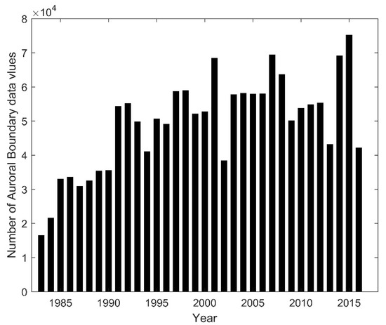
Figure 2.
Number of Auroral Boundary (AB) data values per year in the original ABI data files available in yearly ascii files at the CEDAR Madrigal Archive at http://cedar.openmadrigal.org (accessed on 17 April 2020).
The area encircled by the equatorward auroral boundary, A, which includes the auroral oval plus the polar cap, can be readily estimated from AB. Considering that the auroral equatorward boundary is nearly circular when drawn in CGM for all levels of auroral activity (Madden and Gussenhoven, 1990), the formula of a spherical cap area centered at the geomagnetic pole and limited by the geomagnetic latitude delineated by AB is
This formula is not adequate if geographic coordinates are considered because the geographic latitude of the auroral equatorward boundary varies with longitude, as can be seen in Figure 1a,c. In addition, the oval shape of auroral boundaries in geographic coordinates (especially in the northern hemisphere) turns into circular in CGM.
For each AB data, we interpolated the original Kp index extracted from NASA/GSFC’s OMNI data set through OMNIWeb. In this Kp series, which, as already mentioned, has 8 data per day, the scale 0, 0+, 1−, 1, 1+, 2−, 2, ..., 9 is replaced by 0, 0.3, 0.7, 1, 1.3, 1.7, 2, ..., 9.
3. AB Filtering
Our proposed method to extract changes that originate from the geomagnetic secular variation of the core field consists of four successive steps:
- Filtering of geomagnetic activity.
- Filtering of solar activity.
- Removal of remaining high-frequency signal by a low-order polynomial fit.
- Removal of a dominant solar periodicity by a fit of an oscillatory function.
In the first step, we filter geomagnetic activity from the original data series. We present two different types of filters encompassing four eventual proposed filters. The linear correlation coefficient between AB and Kp, considering the raw data, is greater than 0.6. We then selected AB by classifying the data according to Kp values in the following intervals: 0 < Kp ≤ 2, 2 < Kp ≤ 4, and 4 < Kp ≤ 6. Annual means are then assessed for each case.
We also filter the Kp effect from AB using the complete data set by calculating the residuals from a linear fit between AB and Kp, that is
where a and b are linear regression coefficients between AB and Kp. The effect of the magnetic local time contributes to a large data dispersion, as can be seen in Figure 3a that shows AB vs. Kp for the northern hemisphere as an example. This data dispersion is significantly reduced by considering daily means, as shown in Figure 3b, leading to a linear correlation coefficient between AB and Kp greater than 0.9 for both hemispheres. The red line corresponds to the linear fit, and the departure of AB from this line corresponds to ∆AB of Equation (2), i.e., the filtered series.
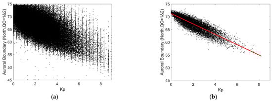
Figure 3.
AB in degrees (°) vs. Kp for the northern hemisphere for data with QC = 1 & 2 during the period 1983–2016 considering the original data (a) and the daily means (b). The linear fit for the daily means (b) is in red.
In the second step, we filter solar activity. This additional source is expected to produce the same effect at both hemispheres: higher solar activity levels are associated with stronger and more frequent geomagnetic storms, implying larger polar caps and auroral ovals in both hemispheres, whereas lower solar activity has the opposite effect. Figure 4 shows the solar activity indicator Rz 11-year running mean, Rz11, which reaches only until 2015 due to the 11-year average process that cuts the last five years at each end of the original series [41,42]. It clearly shows the already mentioned Gleissberg cycle, which is a solar secular variation. A clear long-term decrease in solar activity during the studied period 1983–2015 (enclosed by the red dashed vertical lines) can be noticed in this figure.
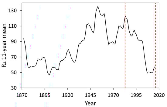
Figure 4.
Sunspot number, Rz, 11-year running mean. Years 1983 and 2016 are indicated as vertical dashed red lines. Data obtained from WDC-SILSO, Royal Observatory of Belgium, Brussels (http://www.sidc.be/silso/datafiles, accessed on 17 April 2020).
We filter this secular trend of solar origin from filtered AB and A annual series through the residuals of a linear fit between each filtered series and Rz 11-year running mean series, that is
where we use double ∆ to emphasize the second filtering.
In the third step, remaining high frequency (typical periods of less than five years) variations in the double-filtered time series of AB, which are unlikely to originate from the slowly varying Earth’s core field, were filtered by a 4th-order polynomial fit. The long-term variation of A is obtained directly in the first three filtered AB series (i.e., the three Kp ranges) of each hemisphere using Equation (1) to convert filtered AB to filtered A. In the fourth filtered AB series (i.e., the Kp linear residuals) of each hemisphere, it is necessary to convert AB to A before the filtering process and then proceed with the filtering considering A instead of AB.
Finally, we will show that there remains a dominant 20–30-year period even after these three steps. This signal may correspond to the ~22-year solar magnetic cycle [43,44], i.e., each quasi-decadal cycle of solar activity has opposed magnetic polarity. However, this periodicity is not regular, alternating between long and short cycles as described by the so-called Gnevyshev–Ohl rule of sunspot number cycles [45,46]. In addition, it has been shown by some authors that geomagnetic activity also presents a ~30-year cycle [47,48]. To remove this dominant external signal, in our fourth step, we estimated the residuals between the 4th-order polynomial of each ∆(∆A) series and a fit with a single frequency of the form
where the fitting parameters are the mean level , the amplitudes and , and the frequency . The obtained fitted periodicity indeed corresponds to a ~20–30-year period oscillation.
4. Results
Annual means of the four AB and A filtered series are plotted in Figure 5 and Figure 6 for the northern and southern hemispheres, respectively. The amplitudes in Figure 5a–c and Figure 6a–c, which correspond to AB data separated for Kp in the ranges 0–2, 2–4, and 4–6, show clearly how, on average, AB value decreases with Kp index. This is consistent with a remarkable shift of the auroral outer boundary towards lower latitudes with increasing geomagnetic activity (as measured by the increase in Kp index)—the auroral zone plus polar cap areas with Kp in the range 4–6 (Figure 5c and Figure 6c) are about ~50% larger than those with the range 0–2 (Figure 5a and Figure 6a). In contrast, the temporal trends of AB are similar in all cases for the northern hemisphere, exhibiting a long-term increase with some flattening towards the present (Figure 5). The same applies to A, for which its behavior was almost identical to AB, but inverse. In the southern hemisphere (Figure 6), AB long-term decrease was much less steep, or even null, with stronger relative interannual variability in almost all cases.
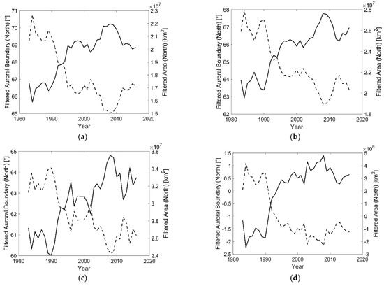
Figure 5.
Northern hemisphere filtered AB (°) time variation considering data with QC = 1 and 2 (solid lines) and corresponding auroral outer boundary enclosed area A (km2) (dashed lines) using the following filters for AB and A: data for 0 < Kp ≤ 2 (a), 2 < Kp ≤ 4 (b), 4 < Kp ≤ 6 (c), and annual means of residuals from the linear regression with Kp (d). Note the different scales.
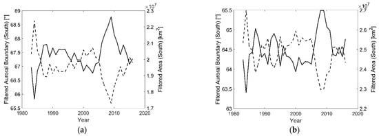
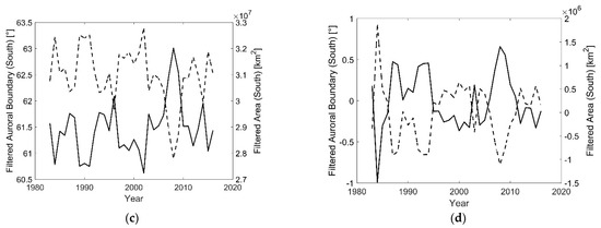
Figure 6.
As in Figure 5 for the Southern hemisphere.
Next, the long-term variation of solar activity was accounted for. We applied a second filter to the AB and A filtered series shown in Figure 5 and Figure 6 based on the long-term variation of solar activity (Equation (3)). The resulting impact of this second filter, shown in Figure 7 and Figure 8 (black lines), is significant. The decreasing areas with time in the northern hemisphere (Figure 5) and the interannual variability in the southern hemisphere (Figure 6) after the first filter both turn to multi-decadal oscillatory trends in Figure 7 and Figure 8.
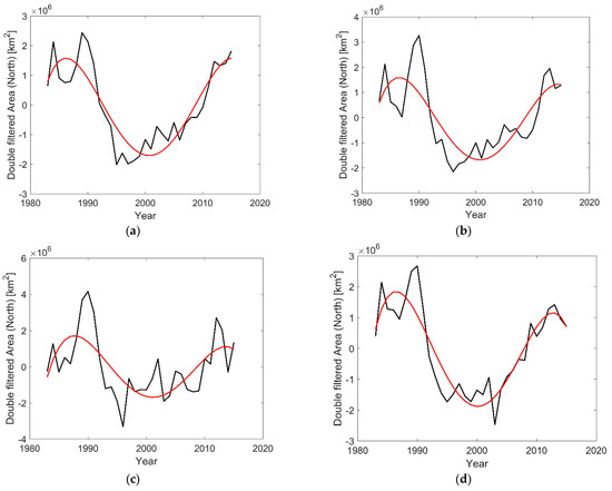
Figure 7.
Northern hemisphere auroral outer boundary enclosed area A (km2) time variation considering AB data with QC = 1 and 2 after filtering secular solar activity variation (black lines), and 4th-order polynomial fits (red lines), from the following filtered data series: AB data converted to A for 0 < Kp ≤ 2 (a), 2 < Kp ≤ 4 (b), 4 < Kp ≤ 6 (c), annual means of AB converted to A residuals from the linear regression with Kp (d). Note the different scales.
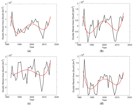
Figure 8.
As in Figure 7 for the Southern hemisphere.
The third step consists of filtering the remaining high-frequency signal. This is applied by a 4th-order polynomial fit to the double-filtered time series, shown as red lines in Figure 7 and Figure 8 for A of each hemisphere. The order 4 truncation of the polynomial fit was chosen because the misfit is asymptotic for higher orders (5 and 6). Adding further terms (7 and 8) revealed the high-frequency signal that is unlikely to originate from the core field. In general, the fit in the northern hemisphere (Figure 7) is better than in the southern (Figure 8).
Finally, the dominant ~20 to ~30-year periodicity, which can be clearly noticed in Figure 7 and Figure 8, is filtered using a single periodicity fit (Equation (4)). The obtained periodicities vary between 26 and 29 years in the northern hemisphere fits, being 29.2, 28.6, 25.9, and 27.3 years in each case considered, that is A for 0 < Kp ≤ 2, for 2 < Kp ≤ 4, for 4 < Kp ≤ 6, and A residuals from the linear regression with Kp, respectively. In the southern case, these periodicities vary between 17 and 20 years, being 17.6, 18.3, 20.2, and 17.7 for the respective cases.
After removing the dominant oscillatory term, we obtain our final results for the auroral oval area estimates of geomagnetic core field origin. These time series are then compared with the model results of Zossi et al. [11]. Figure 9 shows the modeled areas of Zossi et al. [11] separately for the northern and southern hemispheres and superposed the long-term variation of A inferred from observed AB. The area mean value estimated from the modelled area for the period 1983–2015 was added to each of the latter series. The different observation-based time series exhibit similar temporal variability. In the northern hemisphere, the estimates based on low range Kp values (magenta and red lines in Figure 9a) are in better agreement with the model-based time series (thick black line in Figure 9a) than the other two estimates. In the southern hemisphere, the amplitudes of two of the observation-based time series are smaller hence closer to the modeled curve (red and green lines in Figure 9b) while one time series is somewhat off-phase with the others (blue line in Figure 9b).
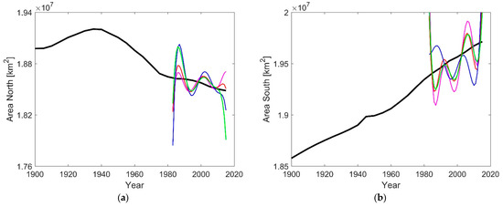
Figure 9.
(a) Northern and (b) southern areas of auroral zone plus polar cap (thick black lines) estimated with a geomagnetic core field model (IGRF 12; Thébault et al., 2015) by Zossi et al. (2020) and corresponding estimates from filtered AB data (this study) considering the following first filters: AB data for 0 < Kp ≤ 2 (magenta), 2 < Kp ≤ 4 (red), 4 < Kp ≤ 6 (blue), annual means of the residuals from the linear regression with Kp (green).
Apart from the severe edge effects due to the Gibbs phenomenon for Fourier-like fits, the long-term trends in the observed northern and southern hemispheres A series are in decent agreement with the model of Zossi et al. [11] for the analyzed period. In both hemispheres, the trends of the temporal variability are in agreement between the observations and the models, i.e., increase in the south (as expected for a geomagnetic dipole decrease) and somewhat surprisingly decrease in the north. The corresponding observed vs. modeled rates are also roughly comparable in each hemisphere. Finally, despite all our filtering efforts, some oscillatory variability appears in the observed signal which is absent in the modeled area. We will discuss below two main possible causes for this discrepancy.
5. Discussion
In this paper we have undertaken the challenging task of isolating a low amplitude signal from an observed time series. The contributions from the sun obscure the slow-varying, low-amplitude geomagnetic core field contribution to auroral zone areas. Indeed, based on the high correlation coefficient between daily AB and Kp, the solar origin forcing determines more than 80% of the variability of AB. In addition, the solar forcing presents not only high-frequency variations but also long-term cycles as well which require much longer time series to be adequately filtered. Overall, this task requires a careful filtering process.
The ability to separate the secular variation in a data series into two different independent sources, internal and external, depends on the relative sizes of each source and on the phase difference between them. If one source produces a significantly weaker signal, it is more difficult to isolate it. In-phase sources cannot be distinguished. To make progress, some knowledge of the underlying physics of each source, e.g., the solar Gleissberg cycle, may allow to separate them. Thus, apart from additional observations, theoretical estimates of the size and phase of AB variation due to the internal geomagnetic field source exclusively may improve the recovery of the modeled trend obtained by Zossi et al. [11].
One step of our procedure involves filtering the dominant 20 to 30-year oscillation attributed to external sources. Although the 11-year oscillation has a larger amplitude, it is removed by the Kp filtering. A combination of a long-term internal secular variation and an external inter-decadal oscillation was also proposed to main field models [49] and their dipole component [50]. The difference is that the main field model (e.g., gufm1 of Jackson et al. [51]) is designed to capture the core field and, as such, is dominantly internal with a very small external residual. In contrast, the AB signal is dominantly external with a small internal part which we attempt to extract.
Any signal can be generically decomposed into oscillatory and non-oscillatory parts. The most naive assumption for the non-oscillatory part is linear. A Fourier series commonly expresses the oscillatory part. In our case, a Fourier series is not applicable because the period of available data is comparable to the dominant periodicity, i.e., the data period is too short. Instead, we fit and remove a single oscillation of a particular periodicity that is well-known to originate from the sun.
Our main results inferred from the AB observations are in decent agreement with Zossi et al. [11] results based on a geomagnetic core field model. We recover the overall decreasing/increasing trends in the northern/southern hemispheres, respectively, with roughly correct rates. In particular, this encouraging agreement provides observational evidence for the surprising recent decrease of the northern auroral zone area. Furthermore, because Zossi et al. [11] interpreted the secular variation of the auroral zone areas in terms of non-dipole field changes, the agreement indicates that the AB data is also affected by the non-dipole field.
It is important to note that among the 13 sites used to derive the Kp index, 11 belong to the northern hemisphere while only two are in the southern (Australia and New Zealand). Even though the correlations between Kp and AB are very similar in both hemispheres, this might contribute to some discrepancies between the south and the north.
Despite our laborious filtering process, our estimated secular variation of auroral zone plus polar cap areas presents a high-frequency variation (Figure 9) which is absent in the modeled area time variation of Zossi et al. [11]. We envision two possible reasons for this discrepancy. First, the over-simplified magnetopause model of Zossi et al. [11] biases the auroral zone areas. Alternatively, because our filtering scheme is imperfect, some solar signal remains. Calculation of auroral zone areas with self-consistent MHD simulations may shed light on the possibility of such high-frequency core-driven oscillations.
Author Contributions
All authors have contributed to the design of this work and to the data and results interpretation. Conceptualization, B.Z. and H.A.; Software and theoretical results, B.Z.; Statistical data analysis, A.G.E.; Formal analysis and investigation, B.Z., H.A., M.F., and A.G.E.; Original draft preparation, A.G.E., B.Z. and M.F.; Review and editing, H.A. All authors have read and agreed to the published version of the manuscript.
Funding
This research was funded by Projects PICT 2018-04447, PIUNT E642, and PIP 294/14.
Institutional Review Board Statement
Not applicable.
Informed Consent Statement
Not applicable.
Data Availability Statement
The Auroral Boundary Index (ABI) was downloaded from Madrigal Database (http://cedar.openmadrigal.org (accessed on 17 April 2020)). Rz data was obtained from WDC-SILSO, Royal Observatory of Belgium, Brussels (http://www.sidc.be/silso/datafiles (accessed on 17 April 2020)), and Kp index from NASA/GSFC’s OMNI data set through OMNIWeb (https://omniweb.gsfc.nasa.gov/ (accessed on 6 July 2021)).
Acknowledgments
We thank four anonymous reviewers for their constructive comments. B.S. Zossi, M. Fagre, and A.G. Elias acknowledge Projects PICT 2018-04447, PIUNT E642, and PIP 294/14. The DMSP particle detectors were designed by Dave Hardy of the Air Force Research Laboratory, and the Auroral Boundary Indices are provided with permission from the Space Vehicle Directorate, Air Force Research Laboratory, Kirtland AFB, NM 87117, via the CEDAR Archival Madrigal Database at Millstone Hill, MIT which the National Science Foundation supports. We acknowledge the use of NASA/GSFC’s Space Physics Data Facility’s OMNIWeb service and OMNI data.
Conflicts of Interest
The authors declare no conflict of interest.
References
- Akasofu, S.I. Evolution of ideas in solar-terrestrial physics. Geophys. J. R. Astron. Soc. 1983, 74, 257–299. [Google Scholar] [CrossRef]
- Feldstein, Y.I. The discovery and the first studies of the auroral oval: A review. Geomagn. Aeron. 2016, 56, 129–142. [Google Scholar] [CrossRef]
- Heirtzler, J.R. The future of the South Atlantic Anomaly and implications for radiation damage in space. J. Atmos. Solar Terr. Phys. 2002, 64, 1701–1708. [Google Scholar] [CrossRef]
- Olson, P.; Amit, H. Changes in earth’s dipole. Naturwissenschaften 2006, 93, 519–542. [Google Scholar] [CrossRef]
- Riley, P.; Baker, D.; Liu, Y.D.; Verronen, P.; Singer, H.; Güdel, M. Extreme Space Weather Events: From Cradle to Grave. Space Sci. Rev. 2018, 214, 21. [Google Scholar] [CrossRef]
- Boteler, D.H. A 21st century view of the March 1989 magnetic storm. Space Weather 2019, 17, 1427–1441. [Google Scholar] [CrossRef]
- Hayakawa, H.; Ribeiro, P.; Vaquero, J.M.; Gallego, M.C.; Knipp, D.J.; Mekhaldi, F.; Bhaskar, A.; Oliveira, D.M.; Notsu, Y.; Carrasco, V.M.S.; et al. The Extreme Space Weather Event in 1903 October/November: An Outburst from the Quiet Sun. Astrophys. J. Lett. 2020, 897, L10. [Google Scholar] [CrossRef]
- Hayakawa, H.; Ribeiro, J.R.; Ebihara YCorreia, A.P.; Sôma, M. South American auroral reports during the Carrington storm. Earth Planets Space 2020, 72, 122. [Google Scholar] [CrossRef]
- Korte, M.; Stolze, S. Variations in Mid-Latitude Auroral Activity During the Holocene. Archaeometry 2016, 58, 159–176. [Google Scholar] [CrossRef]
- Tsyganenko, N.A. Secular drift of the auroral ovals: How fast do they actually move? Geophys. Res. Lett. 2019, 46, 3017–3023. [Google Scholar] [CrossRef]
- Zossi, B.; Fagre, M.; Amit, H.; Elias, A.G. Geomagnetic field model indicates shrinking northern auroral oval. J. Geophys. Res. 2020, 125, e2019JA027434. [Google Scholar] [CrossRef]
- Yokoyama, N.; Kamide, Y.; Miyaoka, H. The size of the auroral belt during magnetic storms. Ann. Geophys. 1998, 16, 566–573. [Google Scholar] [CrossRef]
- Hayakawa, H.; Ebihara, Y.; Willis, D.M.; Toriumi, S.; Iju, T.; Hattori, K.; Wild, M.N.; Oliveira, D.M.; Ermolli, I.; Ribeiro, J.R.; et al. Temporal and spatial evolutions of a large sunspot group and great auroral storms around the Carrington event in 1859. Space Weather 2019, 17, 1553–1569. [Google Scholar] [CrossRef]
- Blake, S.P.; Pulkkinen, A.; Schuck, P.W.; Glocer, A.; Tóth, G. Estimating maximum extent of auroral equatorward boundary using historical and simulated surface magnetic field data. J. Geophys. Res. 2021, 126, e2020JA028284. [Google Scholar] [CrossRef]
- Silverman, S.M. Secular variation of the aurora for the past 500 years. Rev. Geophys. 1992, 30, 333–351. [Google Scholar] [CrossRef]
- Hayakawa, H.; Tamazawa, H.; Ebihara, Y.; Miyahara, H.; Kawamura, A.D.; Aoyama, T.; Isobe, H. Records of sunspots and aurora candidates in the Chinese official histories of the Yuán and Míng dynasties during 1261–1644. Publ. Astron. Soc. Jpn. 2017, 69, 65. [Google Scholar] [CrossRef]
- Silverman, S.; Hayakawa, H. The Dalton Minimum and John Dalton’s Auroral Observations. J. Space Weather Space Clim. 2021, 11, 17. [Google Scholar] [CrossRef]
- Glassmeier, K.H.; Tsurutani, B.T. Carl Friedrich Gauss—General Theory of Terrestrial Magnetism—A revised translation of the German text. Hist. Geo Space. Sci. 2014, 5, 11–62. [Google Scholar] [CrossRef]
- Gubbins, D. Mechanism for geomagnetic polarity reversals. Nature 1987, 326, 167–169. [Google Scholar] [CrossRef]
- Finlay, C.C. Historical variation of the geomagnetic axial dipole. Phys. Earth Planet. Inter. 2008, 170, 1–14. [Google Scholar] [CrossRef]
- Huguet, L.; Amit, H.; Alboussière, T. Geomagnetic dipole changes and upwelling/ downwelling at the top of the Earth’s core. Front. Earth Sci. 2018, 6, 170. [Google Scholar] [CrossRef]
- Siscoe, G.L.; Chen, C.K. The paleomagnetosphere. J. Geophys. Res. 1975, 80, 4575–4680. [Google Scholar] [CrossRef]
- Vogt, J.; Glassmeier, K.H. Modelling the paleomagnetosphere: Strategy and first results. Adv. Space Res. 2001, 28, 863–868. [Google Scholar] [CrossRef]
- Glassmeier, K.H.; Vogt, J.; Stadelmann, A.; Buchert, S. Concerning long-term geomagnetic variations and space climatology. Ann. Geophys. 2004, 22, 3669–3677. [Google Scholar] [CrossRef]
- Schulz, M. Direct influence of ring current on auroral oval diameter. J. Geophys. Res. 1997, 102, 14149–14154. [Google Scholar] [CrossRef]
- Thébault, E.; Finlay, C.C.; Beggan, C.; Alken, P.; Aubert, J.; Barrois, O.; Bertrand, F.; Bondar, T.; Boness, A.; Brocco, L.; et al. International Geomagnetic Reference Field: The 12th generation. Earth Planets Space 2015, 67, 79. [Google Scholar] [CrossRef]
- Gussenhoven, M.S.; Hardy, D.A.; Burke, W.J. DMSP/F2 electron observations of equatorward auroral boundaries and their relationship to magnetospheric electric fields. J. Geophys. Res. 1981, 86, 768–778. [Google Scholar] [CrossRef]
- Gussenhoven, M.S.; Hardy, D.A.; Heinemann, N.; Holeman, E. Diffuse Auroral Boundaries and a Derived Auroral Boundary Index; ADA130175; Air Force Geophysics Laboratory: Hanscom AFB, MA, USA, 1982. [Google Scholar]
- Gussenhoven, M.S.; Hardy, D.A.; Heinemann, N. Systematics of the equatorward diffuse auroral boundary. J. Geophys. Res. 1983, 88, 5692–5708. [Google Scholar] [CrossRef]
- Usoskin, I.G.; Arlt, R.; Asvestari, E.; Hawkins, E.; Käpylä, M.; Kovaltsov, G.A.; Krivova, N.; Lockwood, M.; Mursula, K.; O’Reilly, J.; et al. The Maunder minimum (1645–1715) was indeed a grand minimum: A reassessment of multiple datasets. Astron. Astrophys. 2015, 581, A95. [Google Scholar] [CrossRef]
- Cliver, E.W. Solar Activity and Geomagnetic Storms: The First 40 Years. Eos Trans. AGU 1994, 75, 569–575. [Google Scholar] [CrossRef]
- Demetrescu, C.; Dobrica, V.; Mares, G. On the long-term variability of the heliosphere–magnetosphere environment. Adv. Space Res. 2010, 46, 1299–1310. [Google Scholar] [CrossRef]
- Georgieva, K.; Kirov, B. Solar dynamo and geomagnetic activity. J. Atmos. Solar Terr. Phys. 2011, 73, 207–222. [Google Scholar] [CrossRef]
- Demetrescu, C.; Dobrica, V. The geomagnetic dipole evolution in the last 400 years. Sub-centennial oscillations. In Proceedings of the GEOSCIENCE International Symposium, Bucharest, Romania, 20–22 November 2020; Chitea, F., Ed.; House of the Romanian Academy: Bucarest, Romania, 2021. [Google Scholar]
- Feynman, J.; Ruzmaikin, A. The Centennial Gleissberg Cycle and its association with extended minima. J. Geophys. Res. 2014, 119, 6027–6041. [Google Scholar] [CrossRef]
- Elias, A.G. Filtering ionosphere parameters to detect trends linked to anthropogenic effects. Earth Planets Space 2014, 66, 113. [Google Scholar] [CrossRef]
- Hardy, D.A.; Gussenhoven, M.S.; Holeman, E. A Statistical Model of Auroral Electron Precipitation. J. Geophys. Res. 1985, 90, 4229–4248. [Google Scholar] [CrossRef]
- Madden, D.; Gussenhoven, M.S. Auroral Boundary Index from 1983 to 1990; ADA232845; Space Physics Division, Geophysics Laboratory: Hanscom AFB, MA, USA, 1990. [Google Scholar]
- Schumaker, T.L.; Hardy, D.A.; Moran, S.; Huber, A.; McGarity, J.; Pantazis, J. Precipitating Ion and Electron Detectors (S/4) for the Block 5D/Flight 8 DMSP Satellite; ADA203990; Air Force Geophysics Laboratory: Hanscom AFB, MA, USA, 1988. [Google Scholar]
- Gustafsson, G.; Papitashvili, N.E.; Papitashvili, V.O. A Revised Corrected Geomagnetic Coordinate System for Epochs 1985 and 1990. J. Atmos. Terr. Phys. 1992, 54, 1609–1631. [Google Scholar] [CrossRef]
- Clette, F.; Svalgaard, L.; Vaquero, J.M.; Cliver, E.W. Revisiting the Sunspot Number. Space Sci. Rev. 2014, 186, 35–103. [Google Scholar] [CrossRef]
- Clette, F.; Lefevre, L. The New Sunspot Number: Assembling All Corrections. Sol. Phys. 2016, 291, 2629–2651. [Google Scholar] [CrossRef]
- Cliver, E.W.; Boriakoff, V.; Bounar, K.H. The 22-year cycle of geomagnetic and solar wind activity. J. Geophys. Res. 1996, 101, 27091–27109. [Google Scholar] [CrossRef]
- Hathaway, D.H. The Solar Cycle. Living Rev. Sol. Phys. 2015, 12, 4. [Google Scholar] [CrossRef]
- Tlatov, A.G. Reversals of Gnevyshev-Ohl rule. Astrophys. J. Lett. 2013, 772, L30. [Google Scholar] [CrossRef][Green Version]
- Zolotova, N.V.; Ponyavin, D.I. The Gnevyshev-Ohl rule and its violations. Geomagn. Aeron. 2015, 55, 902–906. [Google Scholar] [CrossRef]
- Rangarajan, G.K.; Iyemori, T. Time variations of geomagnetic activity indices Kp and Ap: An update. Ann. Geophys. 1997, 15, 1271–1290. [Google Scholar] [CrossRef]
- Komitov, B.; Sello, S.; Duchlev, P.; Dechev, M.; Penev, K.; Koleva, K. Sub- and Quasi-Centurial Cycles in Solar and Geomagnetic Activity Data Series. Bulg. Astron. J. 2016, 25, 78–103. [Google Scholar]
- Dobrica, V.; Stefan, C.; Demetrescu, C. Planetary scale geomagnetic secular variation foci in the last 400 years. Glob. Planet. Chang. 2021, 199, 103430. [Google Scholar] [CrossRef]
- Demetrescu, C.; Dobrica, V. Signature of Hale and Gleissberg solar cycles in the geomagnetic activity. J. Geophys. Res. 2008, 113, A02103. [Google Scholar] [CrossRef]
- Jackson, A.; Jonkers, A.; Walker, M. Four centuries of geomagnetic secular variation from historical records. Phil. Trans. R. Soc. 2000, 358, 957–990. [Google Scholar] [CrossRef]


Publisher’s Note: MDPI stays neutral with regard to jurisdictional claims in published maps and institutional affiliations. |
© 2021 by the authors. Licensee MDPI, Basel, Switzerland. This article is an open access article distributed under the terms and conditions of the Creative Commons Attribution (CC BY) license (https://creativecommons.org/licenses/by/4.0/).