
Multiscale Characterisation of Fracture Patterns of a Crystalline Reservoir Analogue


Abstract
:1. Introduction
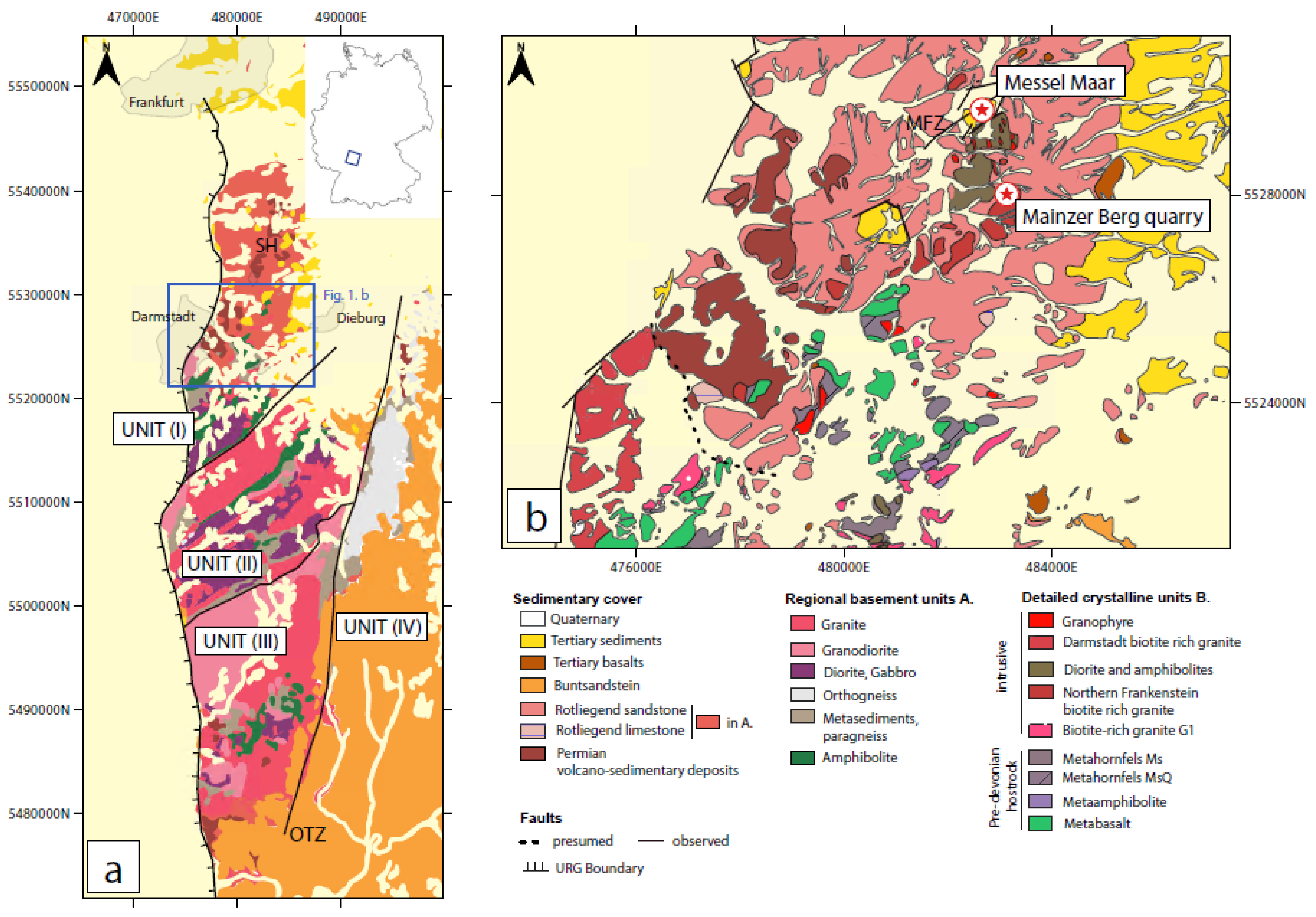
2. Geological Context
3. Materials and Methods
4. Results
4.1. Regional Lineaments
4.2. LiDAR Imaging at the Outcrop Scale of the Structural Network
4.3. GIS Structural Analysis of Profiles
4.4. Fault Zone Domains
5. Discussion
5.1. Clustering of the Fracture Network
5.2. Topology of the Fracture Network, Influence on Connectivity and Flow Properties
5.3. Multiscale Laws of Fault and Fracture Network in Granitic and Granodioritic Units
5.4. Conceptual Granitic Reservoir Model from the Analogue
6. Conclusions
Supplementary Materials
Author Contributions
Funding
Data Availability Statement
Acknowledgments
Conflicts of Interest
References
- Vidal, J.; Genter, A. Overview of naturally permeable fractured reservoirs in the central and southern Upper Rhine Graben: Insights from geothermal wells. Geothermics 2018, 74, 57–73. [Google Scholar] [CrossRef]
- Place, J.; Géraud, Y.; Diraison, M.; Herquel, G.; Edel, J.B.; Bano, M.; Le Garzic, E.; Walter, B. Structural control of weathering processes within exhumed granitoids: Compartmentalisation of geophysical properties by faults and fractures. J. Struct. Geol. 2016, 84, 102–119. [Google Scholar] [CrossRef]
- Bertrand, L.; Jusseaume, J.; Géraud, Y.; Diraison, M.; Damy, P.C.; Navelot, V.; Haffen, S. Structural heritage, reactivation and distribution of fault and fracture network in a rifting context: Case study of the western shoulder of the Upper Rhine Graben. J. Struct. Geol. 2018, 108, 243–255. [Google Scholar] [CrossRef]
- Aquilina, L.; Boulvais, P.; Mossmann, J.R. Fluid migration at the basement/sediment interface along the margin of the Southeast basin (France): Implications for Pb-Zn ore formation. Miner. Depos. 2011, 46, 959–979. [Google Scholar] [CrossRef]
- Meixner, J.; Schill, E.; Grimmer, J.C.; Gaucher, E.; Kohl, T.; Klingler, P. Structural control of geothermal reservoirs in extensional tectonic settings: An example from the Upper Rhine Graben. J. Struct. Geol. 2016, 82, 1–15. [Google Scholar] [CrossRef]
- Meixner, J.; Grimmer, J.C.; Becker, A.; Schill, E.; Kohl, T. Comparison of different digital elevation models and satellite imagery for lineament analysis: Implications for identification and spatial arrangement of fault zones in crystalline basement rocks of the southern Black Forest (Germany). J. Struct. Geol. 2018, 108, 256–268. [Google Scholar] [CrossRef]
- Meller, C.; Schill, E.; Bremer, J.; Kolditz, O.; Bleicher, A.; Benighaus, C.; Chavot, P.; Gross, M.; Pellizzone, A.; Renn, O.; et al. Acceptability of geothermal installations: A geoethical concept for GeoLaB. Geothermics 2018, 73, 133–145. [Google Scholar] [CrossRef]
- Dezayes, C.; Lerouge, C. Reconstructing Paleofluid Circulation at the Hercynian Basement/Mesozoic Sedimentary Cover Interface in the Upper Rhine Graben. Geofluids 2019, 2019, 4849860. [Google Scholar] [CrossRef]
- Baujard, C.; Genter, A.; Dalmais, E.; Maurer, V.; Hehn, R.; Rosillette, R.; Vidal, J.; Schmittbuhl, J. Hydrothermal characterization of wells GRT-1 and GRT-2 in Rittershoffen, France: Implications on the understanding of natural flow systems in the rhine graben. Geothermics 2017, 65, 255–268. [Google Scholar] [CrossRef] [Green Version]
- Glaas, C.; Vidal, J.; Genter, A. Structural characterisation of naturally fractured geothermal reservoirs in the central Upper Rhine Graben. J. Struct. Geol. 2021, 148, 104370. [Google Scholar] [CrossRef]
- Stober, I.; Bucher, K. Hydraulic and hydrochemical properties of deep sedimentary reservoirs of the Upper Rhine Graben, Europe. Geofluids 2015, 15, 464–482. [Google Scholar] [CrossRef]
- Kushnir, A.R.L.; Heap, M.J.; Baud, P.; Gilg, H.A.; Reuschlé, T.; Lerouge, C.; Dezayes, C.; Duringer, P. Characterising the physical properties of rocks from the Paleozoic to Permo-Triassic transition in the Upper Rhine Graben. Geotherm. Energy 2018, 6, 16. [Google Scholar] [CrossRef]
- Koltzer, N.; Scheck-wenderoth, M.; Bott, J.; Cacace, M.; Frick, M.; Sass, I.; Fritsche, J.; Bär, K. The Effect of Regional Fluid Flow on Deep temperatures (Hesse, Germany). Energies 2019, 12, 2081. [Google Scholar] [CrossRef] [Green Version]
- McCaffrey, K.J.W.; Holdsworth, R.E.; Pless, J.; Franklin, B.S.G.; Hardman, K. Basement reservoir plumbing: Fracture aperture, length and topology analysis of the Lewisian Complex, NW Scotland. J. Geol. Soc. Lond. 2020, 177, 1281–1293. [Google Scholar] [CrossRef]
- Stein, E. The geology of the Odenwald Crystalline Complex. Mineral. Petrol. 2001, 72, 7–28. [Google Scholar] [CrossRef]
- Kirsch, H.; Kober, B.; Lippolt, H.J. Age of intrusion and rapid cooling of the Frankenstein gabbro (Odenwald, SW-Germany) evidenced by40Ar/39Ar and single-zircon207Pb/206Pb measurements. Geol. Rundsch. 1988, 77, 693–711. [Google Scholar] [CrossRef]
- Dörr, W.; Stein, E. Precambrian basement in the Rheic suture zone of the Central European Variscides (Odenwald). Int. J. Earth Sci. 2019, 108, 1937–1957. [Google Scholar] [CrossRef]
- Krohe, A. Structural evolution of intermediate-crustal rocks in a strike-slip and extensional setting (Variscan Odenwald, SW Germany): Differential upward transport of metamorphic complexes and changing deformation mechanisms. Tectonophysics 1992, 205, 357–386. [Google Scholar] [CrossRef]
- Will, T.M.; Schulz, B.; Schmädicke, E. The timing of metamorphism in the Odenwald–Spessart basement, Mid-German Crystalline Zone. Int. J. Earth Sci. 2017, 106, 1631–1649. [Google Scholar] [CrossRef]
- Anderle, H.J. The evolution of the South Hunsrück and Taunus Borderzone. Tectonophysics 1987, 137, 101–114. [Google Scholar] [CrossRef]
- Izart, A.; Barbarand, J.; Michels, R.; Privalov, V.A. Modelling of the thermal history of the Carboniferous Lorraine Coal Basin: Consequences for coal bed methane. Int. J. Coal Geol. 2016, 168, 253–274. [Google Scholar] [CrossRef]
- Böcker, J.; Littke, R.; Forster, A. An Overview on Source Rocks and the Petroleum System of the Central Upper Rhine Graben; Springer: Berlin/Heidelberg, Germany, 2016; ISBN 0053101613303. [Google Scholar]
- Bourgeois, O.; Ford, M.; Diraison, M.; Le Carlier de Veslud, C.; Gerbault, M.; Pik, R.; Ruby, N.; Bonnet, S.; de Veslud, C.L.C.; Gerbault, M.; et al. Separation of rifting and lithospheric folding signatures in the NW-Alpine foreland. Int. J. Earth Sci. 2007, 96, 1003–1031. [Google Scholar] [CrossRef]
- Schumacher, M.E. Upper Rhine Graben: Role of preexisting structures during rift evolution. Tectonics 2002, 21, 6-1–6-17. [Google Scholar] [CrossRef]
- Mezger, J.E.; Felder, M.; Harms, F.J. Crystalline rocks in the maar deposits of Messel: Key to understand the geometries of the Messel Fault Zone and diatreme and the post-eruptional development of the basin fill. Z. Dtsch. Ges. Geowiss. 2013, 164, 639–662. [Google Scholar] [CrossRef]
- Lutz, H.; Lorenz, V.; Engel, T.; Häfner, F.; Haneke, J. Paleogene phreatomagmatic volcanism on the western main fault of the northern Upper Rhine Graben (Kisselwörth diatreme and Nierstein-Astheim Volcanic System, Germany). Bull. Volcanol. 2013, 75, 741. [Google Scholar] [CrossRef] [Green Version]
- Ziegler, P.A.; Dèzes, P. Cenozoic uplift of Variscan Massifs in the Alpine foreland: Timing and controlling mechanisms. Glob. Planet. Chang. 2007, 58, 237–269. [Google Scholar] [CrossRef]
- Cloetingh, S.; Cornu, T.; Ziegler, P.A.; Beekman, F.; Ustaszewski, K.; Schmid, S.M.; Dèzes, P.; Hinsch, R.; Decker, K.; Lopes Gardozo, G.; et al. Neotectonics and intraplate continental topography of the northern Alpine Foreland. Earth-Sci. Rev. 2006, 74, 127–196. [Google Scholar] [CrossRef]
- Sissingh, W. Tertiary paleogeographic and tectonostratigraphic evolution of the Rhenish Triple Junction. Palaeogeogr. Palaeoclimatol. Palaeoecol. 2003, 196, 229–263. [Google Scholar] [CrossRef]
- Ford, M.; Le Carlier de Veslud, C.; Bourgeois, O. Kinematic and geometric analysis of fault-related folds in a rift setting: The Dannemarie basin, Upper Rhine Graben, France. J. Struct. Geol. 2007, 29, 1811–1830. [Google Scholar] [CrossRef]
- Dèzes, P.; Schmid, S.M.M.; Ziegler, P.A. Evolution of the European Cenozoic Rift System: Interaction of the Alpine and Pyrenean orogens with their foreland lithosphere. Tectonophysics 2004, 389, 1–33. [Google Scholar] [CrossRef]
- Derer, C.E. Tectono-Sedimentary Evolution of the Northern Upper Rhine Graben (Germany), with Special Regard to the Early syn-Rift Stage. Dissertation 2003, pp. 1–99. Available online: https://bonndoc.ulb.uni-bonn.de/xmlui/handle/20.500.11811/1930 (accessed on 27 August 2021).
- Derer, C.E.; Schumacher, M.E.; Schäfer, A. The northern Upper Rhine Graben: Basin geometry and early syn-rift tectono-sedimentary evolution. Int. J. Earth Sci. 2005, 94, 640–656. [Google Scholar] [CrossRef]
- Gu, Y.; Rühaak, W.; Bär, K.; Sass, I. Using seismic data to estimate the spatial distribution of rock thermal conductivity at reservoir scale. Geothermics 2017, 66, 61–72. [Google Scholar] [CrossRef]
- Molenaar, N.; Felder, M.; Bär, K.; Götz, A.E. What classic greywacke (litharenite) can reveal about feldspar diagenesis: An example from Permian Rotliegend sandstone in Hessen, Germany. Sediment. Geol. 2015, 326, 79–93. [Google Scholar] [CrossRef]
- Thews, J.-D. Erläuterungen zur Geologischen Übersichtskarte von Hessen 1:300000 (GÜK300 Hessen) Teil I: Kristallin, Ordoviz, Silur, Devon, Karbon.- Geologische Abhandlungen von Hessen, Bd. 96, 1996, Hessisches Landesamt für Umwelt und Geologie; Wiesbaden. Available online: https://www.hlnug.de/themen/geologie/geologische-landesaufnahme/produkte/guek300 (accessed on 3 September 2021).
- Frey, M.; Weinert, S.; Bär, K.; van der Vaart, J.; Dezayes, C.; Calcagno, P.; Sass, I. Integrated 3D geological modelling of the northern Upper Rhine Graben by joint inversion of gravimetry and magnetic data. Tectonophysics 2021, 813, 228927. [Google Scholar] [CrossRef]
- Weinert, S.; Bär, K.; Sass, I. Database of petrophysical properties of the Mid-German Crystalline Rise. Earth Syst. Sci. Data 2021, 13, 1441–1459. [Google Scholar] [CrossRef]
- Luby, S.; Geraud, Y.; Diraison, M.; Wicker, M.; Bertrand, L.; Bossennec, C. Multiscale investigation focusing on the lineament of the Pan-African basement (Eastern Egypt). In Proceedings of the Fourth Naturally Fractured Reservoir Workshop, Ras Al Khaimah, United Arab Emirates, 11–13 February 2020; pp. 1–5. [Google Scholar]
- Chabani, A.; Trullenque, G.; Ledésert, B.A.; Klee, J. Multiscale Characterization of Fracture Patterns: A Case Study of the Noble Hills Range (Death Valley, CA, USA), application to geothermal reservoirs. Geosciences 2021, 11, 280. [Google Scholar] [CrossRef]
- Mikita, T.; Balková, M.; Bajer, A.; Cibulka, M.; Patočka, Z. Comparison of different remote sensing methods for 3d modeling of small rock outcrops. Sensors 2020, 20, 1663. [Google Scholar] [CrossRef] [PubMed] [Green Version]
- Zeng, Q.; Lu, W.; Zhang, R.; Zhao, J.; Ren, P.; Wang, B. LIDAR-Based Fracture Characterisation and Controlling Factors Analysis: An Outcrop Case from Kuqa Depression, NW China; Elsevier B.V.: Amsterdam, The Netherlands, 2018; Volume 161, ISBN 0500300100. [Google Scholar]
- Fisher, J.E.; Shakoor, A.; Watts, C.F. Comparing discontinuity orientation data collected by terrestrial LiDAR and transit compass methods. Eng. Geol. 2014, 181, 78–92. [Google Scholar] [CrossRef]
- Vöge, M.; Lato, M.J.; Diederichs, M.S. Automated rockmass discontinuity mapping from 3-dimensional surface data. Eng. Geol. 2013, 164, 155–162. [Google Scholar] [CrossRef]
- Biber, K.; Khan, S.D.; Seers, T.D.; Sarmiento, S.; Lakshmikantha, M.R. Quantitative characterisation of a naturally fractured reservoir analog using a hybrid lidar-gigapixel imaging approach. Geosphere 2018, 14, 710–730. [Google Scholar] [CrossRef]
- Schnabel, R.; Wahl, R.; Klein, R. RANSAC based out-of-core point-cloud shape detection for city-modeling. Proc. Terr. Laserscanning 2007, 26, 214–226. [Google Scholar]
- Bisdom, K.; Gauthier, B.D.M.; Bertotti, G.; Hardebol, N.J. Calibrating discrete fracture-network models with a carbonate three- dimensional outcrop fracture network: Implications for naturally fractured reservoir modeling. AAPG Bull. 2014, 7, 1351–1376. [Google Scholar] [CrossRef]
- Ortega, O.J.; Marrett, R.A.; Laubach, S.E. A scale-independent approach to fracture intensity and average spacing measurement. Am. Assoc. Pet. Geol. Bull. 2006, 90, 193–208. [Google Scholar] [CrossRef]
- Allmendiger, R. Stereonet 11 | Rick Allmendinger’s Stuff. Available online: http://www.geo.cornell.edu/geology/faculty/RWA/programs/stereonet.html (accessed on 27 July 2021).
- Fisher, N.; Lewis, T.; Embleton, B. Statistical Analysis of Spherical Data; Cambridge University Press: Cambridge, UK, 1993. [Google Scholar]
- Peacock, D.C.P.; Dimmen, V.; Rotevatn, A.; Sanderson, D.J. A broader classification of damage zones. J. Struct. Geol. 2017, 102, 179–192. [Google Scholar] [CrossRef]
- Peacock, D.C.P.; Nixon, C.W.; Rotevatn, A.; Sanderson, D.J.; Zuluaga, L.F. Glossary of fault and other fracture networks. J. Struct. Geol. 2016, 92, 12–29. [Google Scholar] [CrossRef]
- Sanderson, D.J.; Nixon, C.W. Topology, connectivity and percolation in fracture networks. J. Struct. Geol. 2018, 115, 167–177. [Google Scholar] [CrossRef]
- Rizzo, R.E.; Healy, D.; Farrell, N.J.; Heap, M.J. Riding the Right Wavelet: Quantifying Scale Transitions in Fractured Rocks. Geophys. Res. Lett. 2017, 44, 11808–11815. [Google Scholar] [CrossRef] [Green Version]
- Putz-Perrier, M.W.; Sanderson, D.J. The distribution of faults and fractures and their importance in accommodating extensional strain at Kimmeridge Bay, Dorset, UK. Geol. Soc. Lond. Spec. Publ. 2008, 299, 97–111. [Google Scholar] [CrossRef]
- Peacock, D.C.P.; Sanderson, D.J.; Rotevatn, A. Relationships between fractures. J. Struct. Geol. 2018, 106, 41–53. [Google Scholar] [CrossRef]
- Gillespie, P.A.; Walsh, J.J.; Watterson, J.; Bonson, C.G.; Manzocchi, T. Scaling relationships of joint and vein arrays from The Burren, Co. Clare, Ireland. J. Struct. Geol. 2001, 23, 183–201. [Google Scholar] [CrossRef]
- Watkins, H.; Bond, C.E.; Healy, D.; Butler, R.W.H. Appraisal of fracture sampling methods and a new workflow tocharacterise heterogeneous fracture networks at outcrop. J. Struct. Geol. 2015, 72, 67–82. [Google Scholar] [CrossRef]
- Sanderson, D.J.; Peacock, D.C.P. Line sampling of fracture swarms and corridors. J. Struct. Geol. 2019, 122, 27–37. [Google Scholar] [CrossRef]
- Bonnet, E.; Bour, O.; Odling, N.E.; Davy, P.; Main, I.; Cowie, P.; Berkowitz, B. Scaling of fracture systems in geological media. Rev. Geophys. 2001, 39, 347–383. [Google Scholar] [CrossRef] [Green Version]
- Primaleon, L.P.; McCaffrey, K.J.W.; Holdsworth, R.E. Fracture attribute and topology characteristics of a geothermal reservoir: Southern negros, philippines. J. Geol. Soc. Lond. 2020, 177, 1092–1106. [Google Scholar] [CrossRef]
- Choi, J.-H.H.; Edwards, P.; Ko, K.; Kim, Y.-S.S. Definition and classification of fault damage zones: A review and a new methodological approach. Earth-Sci. Rev. 2016, 152, 70–87. [Google Scholar] [CrossRef]
- Olson, J.E. Sublinear scaling of fracture aperture versus length: An exception or the rule? J. Geophys. Res. 2003, 108, 2413. [Google Scholar] [CrossRef]
- Odling, N.E.; Gillespie, P.; Bourgine, B.; Castaing, C. Variations in fracture system geometry and their implications for fluid flow in fractured hydrocarbon reservoirs. Pet. Geosci. 1999, 5, 373–384. [Google Scholar] [CrossRef]
- Bertrand, L.; Géraud, Y.; Le Garzic, E.; Place, J.; Diraison, M.; Walter, B.; Haffen, S. A multiscale analysis of a fracture pattern in granite: A case study ofthe Tamariu granite, Catalunya, Spain. J. Struct. Geol. 2015, 78, 52–66. [Google Scholar] [CrossRef]
- Martinelli, M.; Bistacchi, A.; Mittempergher, S.; Bonneau, F.; Balsamo, F.; Caumon, G.; Meda, M. Damage zone characterisation combining scanline and scan-area analysis on a km-scale Digital Outcrop Model: The Qala Fault (Gozo). J. Struct. Geol. 2020, 140, 104144. [Google Scholar] [CrossRef]
- Laubach, S.E.; Lamarche, J.; Gauthier, B.D.M.; Dunne, W.M.; Sanderson, D.J. Spatial arrangement of faults and opening-mode fractures. J. Struct. Geol. 2017, 108, 2–15. [Google Scholar] [CrossRef]
- Bertrand, L.; Géraud, Y.; Diraison, M. Petrophysical properties in faulted basement rocks: Insights from outcropping analogues on the West European Rift shoulders. Geothermics 2021, 95, 102144. [Google Scholar] [CrossRef]
- Liang, F.; Niu, J.; Linsel, A.; Hinderer, M.; Scheuvens, D.; Petschick, R. Rock alteration at the post-Variscan nonconformity: Implications for Carboniferous-Permian surface weathering versus burial diagenesis and paleoclimate evaluation. Solid Earth 2021, 12, 1165–1184. [Google Scholar] [CrossRef]
- Le Garzic, E.; de L’Hamaide, T.; Diraison, M.; Géraud, Y.; Sausse, J.; de Urreiztieta, M.; Hauville, B.; Champanhet, J.M. Scaling and geometric properties of extensional fracture systems in the proterozoic basement of Yemen. Tectonic interpretation and fluid flow implications. J. Struct. Geol. 2011, 33, 519–536. [Google Scholar] [CrossRef]
- McCaffrey, K.J.W.; Sleight, J.M.; Pugliese, S.; Holdsworth, R.E. Fracture formation and evolution in crystalline rocks: Insights from attribute analysis. Geol. Soc. Spec. Publ. 2003, 214, 109–124. [Google Scholar] [CrossRef]
- Žák, J.; Vyhnálek, B.; Kabele, P. Is there a relationship between magmatic fabrics and brittle fractures in plutons?: A view based on structural analysis, anisotropy of magnetic susceptibility and thermo-mechanical modelling of the Tanvald pluton (Bohemian Massif). Phys. Earth Planet. Inter. 2006, 157, 286–310. [Google Scholar] [CrossRef]
- Žák, J.; Verner, K.; Ježek, J.; Trubač, J. Complex mid-crustal flow within a growing granite–migmatite dome: An example from the Variscan belt illustrated by the anisotropy of magnetic susceptibility and fabric modelling. Geol. J. 2019, 54, 3681–3699. [Google Scholar] [CrossRef]
- Zibra, I.; White, J.C.; Menegon, L.; Dering, G.; Gessner, K. The ultimate fate of a synmagmatic shear zone. Interplay between rupturing and ductile flow in a cooling granite pluton. J. Struct. Geol. 2018, 110, 1–23. [Google Scholar] [CrossRef]


| Layer | Min Length (m) | Max Length (m) | Mean Length (m) | a | b | rsq | P20 (lin.m−1) | P21 (m·m−2) |
|---|---|---|---|---|---|---|---|---|
| DEM_25 m (Figure 3a) | 147.68 | 8407.05 | 1341.56 | 1.99 × 10⁻¹ | −1.83 | 0.98 | 1.09 × 10⁻⁶ | 1.46 × 10⁻³ |
| DEM_1 m (Figure 3b) | 50.98 | 5112.83 | 872.77 | 8.50 × 10⁻² | −1.69 | 0.97 | 2.47 × 10⁻⁶ | 2.16 × 10⁻³ |
| Messel_pit (blue, Figure 3c) | 37.47 | 1918.28 | 224.78 | 0.0005 | −1.12 | 0.96 | 3.14 × 10⁻⁵ | 7.06 × 10⁻³ |
| DEM_zoom_1 m | 4.09 | 985.64 | 148.26 | 0.033 | −1.51 | 0.98 | 4.70 × 10⁻⁵ | 6.97 × 10⁻³ |
| Satellite imaging Mainzer Berg (green, Figure 3c) | 4.09 | 356.72 | 66.74 | 0.00189 | −0.83 | 0.96 | 1.89 × 10⁻⁴ | 1.26 × 10⁻² |
| Profile | Min. Length (m) | Max. Length (m) | Mean. Length (m) | a | b | R2 | Density (P30) | Intensity (P32) |
|---|---|---|---|---|---|---|---|---|
| A | 1.85 | 37.37 | 10.98 | 388.5 | −2.69 | 0.99 | 2.07 × 10⁻² | 1.17 |
| B | 0.82 | 15.15 | 3.99 | 32.9 | −3.34 | 0.97 | 3.45 × 10⁻² | 0.33 |
| C | 1.26 | 40.66 | 12.27 | 3863.3 | −3.70 | 0.99 | 3.40 × 10⁻² | 2.51 |
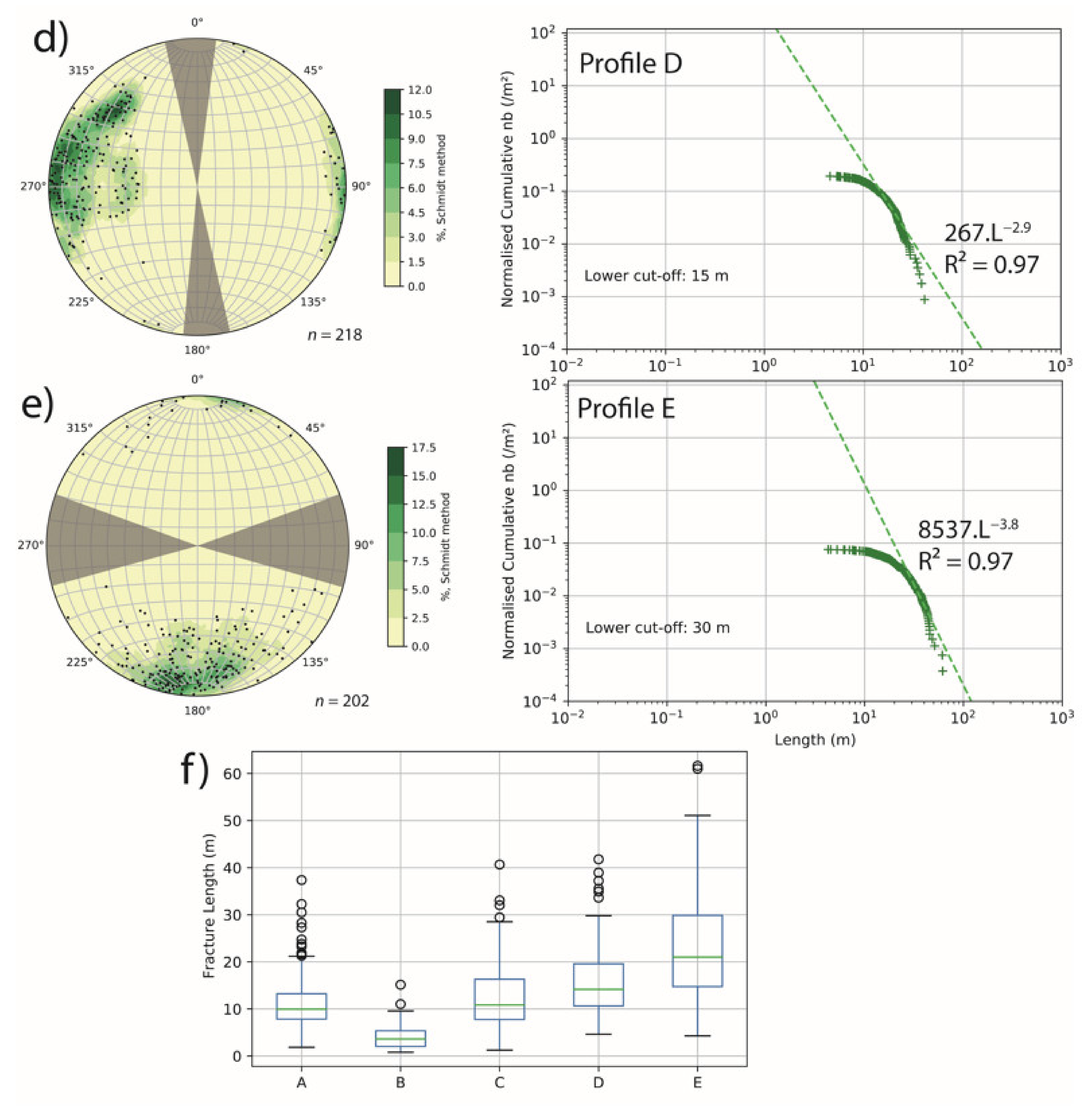
| D | 4.61 | 41.79 | 15.68 | 267.1 | −2.91 | 0.97 | 1.94 × 10⁻³ | 0.25 |
| E | 4.26 | 61.63 | 23.22 | 8537.1 | −3.80 | 0.97 | 4.92 × 10⁻³ | 1.37 |
| Cluster name | Proportion | Trend | Plunge | n | a95 | a99 | kappa | Min. Length (m) | Max. Length (m) | Mean length (m) | a | b | R2 | Density (P30) | Intensity (P32) |
|---|---|---|---|---|---|---|---|---|---|---|---|---|---|---|---|
| C1 | 8.83% | 15.4 | 8 | 95 | 1.5 | 1.8 | 97.4 | 1.21 | 48.44 | 15.95 | 0.052 | −1.404 | 0.939 | 1.28 × 10⁻⁴ | 1.69 × 10⁻² |
| C2 | 3.25% | 352 | 11 | 35 | 2.2 | 2.7 | 125.5 | 5.25 | 45.42 | 20.78 | 0.354 | −2.248 | 0.944 | 4.46 × 10⁻⁵ | 1.15 × 10⁻² |
| C3 | 1.86% | 326.5 | 15.1 | 20 | 2.4 | 3 | 190.2 | 2.84 | 27.39 | 10.20 | 11.014 | −3.866 | 0.952 | 1.67 × 10⁻⁴ | 8.51 × 10⁻³ |
| C4 | 4.65% | 297.8 | 12 | 50 | 2.1 | 2.7 | 89.5 | 5.88 | 28.28 | 13.62 | 0.727 | −2.302 | 0.969 | 2.23 × 10⁻⁴ | 1.78 × 10⁻² |
| C5 | 5.20% | 268.4 | 10.8 | 56 | 1.9 | 2.4 | 96.9 | 3.59 | 35.53 | 17.53 | 0.211 | −1.692 | 0.932 | 2.01 × 10⁻⁴ | 3.25 × 10⁻² |
| C6 | 6.04% | 248.6 | 24.6 | 65 | 2.3 | 2.8 | 61.2 | 7.22 | 29.59 | 14.01 | 0.016 | −1.396 | 0.948 | 5.58 × 10⁻⁵ | 5.96 × 10⁻³ |
| C7 | 6.78% | 203.3 | 36 | 73 | 2.6 | 3.2 | 42.2 | 0.89 | 36.42 | 15.79 | 0.171 | −1.728 | 0.980 | 1.73 × 10⁻⁴ | 2.56 × 10⁻² |
| C8 | 4.28% | 196.9 | 5.7 | 46 | 2.6 | 3.3 | 65.9 | 0.96 | 61.63 | 18.44 | 0.041 | −1.187 | 0.950 | 1.73 × 10⁻⁴ | 3.53 × 10⁻² |
| C9 | 5.76% | 133.5 | 20.9 | 62 | 2.1 | 2.6 | 76.8 | 4.81 | 22.91 | 12.27 | 0.074 | −2.019 | 0.924 | 5.02 × 10⁻⁵ | 4.01 × 10⁻³ |
| C10 | 5.30% | 107.8 | 9.8 | 57 | 2 | 2.4 | 93.7 | 7.04 | 30.50 | 14.18 | 0.989 | −2.465 | 0.936 | 1.79 × 10⁻⁴ | 1.64 × 10⁻² |
| C11 | 3.35% | 84.7 | 8.2 | 36 | 2.2 | 2.8 | 115.5 | 1.74 | 25.76 | 9.95 | 26.417 | −3.857 | 0.988 | 3.57 × 10⁻⁴ | 1.76 × 10⁻² |
| Profile | Layer | Length Min (m) | Length Max (m) | Mean Length (m) | a | b | rsq | Density (P20) | Intensity (P21) | Cut off Value (m) | n Elements | Area (m2) |
|---|---|---|---|---|---|---|---|---|---|---|---|---|
| A | GIS top | 0.17 | 7.08 | 1.38 | 0.760 | −1.705 | 0.983 | 1.22 | 1.69 | 1.0 | 559 | 458 |
| GIS side | 0.48 | 13.90 | 1.97 | 1.135 | −1.945 | 0.992 | 0.89 | 1.75 | 1.5 | 542 | 610 | |
| B | GIS top | 0.18 | 5.32 | 1.26 | 1.008 | −1.846 | 0.997 | 2.02 | 2.54 | 1.0 | 263 | 130 |
| GIS side | 0.17 | 4.73 | 1.01 | 1.057 | −1.709 | 0.993 | 3.21 | 3.26 | 0.7 | 414 | 129 | |
| C | GIS top | 0.03 | 18.03 | 0.88 | 2.118 | −2.921 | 0.981 | 4.12 | 3.63 | 1.5 | 754 | 183 |
| GIS side | 0.04 | 11.68 | 1.01 | 1.124 | −1.547 | 0.993 | 3.44 | 3.49 | 0.7 | 1377 | 400 | |
| D | GIS top | 0.18 | 15.39 | 4.58 | 0.369 | −1.560 | 0.990 | 0.10 | 0.46 | 3.0 | 210 | 2106 |
| GIS side | 1.02 | 32.58 | 5.23 | 0.715 | −1.873 | 0.995 | 0.10 | 0.51 | 3.0 | 380 | 3870 | |
| E | GIS top | 0.28 | 12.81 | 2.38 | 1.259 | −2.082 | 0.995 | 0.58 | 1.39 | 2.0 | 550 | 942 |
| GIS side | 0.50 | 33.47 | 4.22 | 0.274 | −1.945 | 0.992 | 0.20 | 0.86 | 1.5 | 516 | 2525 |
| Section | Ns | Mean P10 | Mean Nf | Mean Cv | Min Cv | Max Cv |
|---|---|---|---|---|---|---|
| C top | 19 | 2.60 | 34.26 | 1.02 | 0.72 | 1.36 |
| C side | 5 | 3.31 | 56.50 | 0.89 | 0.67 | 1.41 |
| D top | 11 | 0.45 | 15.00 | 1.25 | 0.84 | 1.71 |
| D side | 11 | 0.43 | 30.64 | 1.11 | 0.74 | 1.89 |
| E top | 5 | 1.04 | 30.20 | 0.88 | 0.69 | 1.20 |
| E side | 16 | 0.77 | 31.63 | 0.99 | 0.54 | 1.29 |
Publisher’s Note: MDPI stays neutral with regard to jurisdictional claims in published maps and institutional affiliations. |
© 2021 by the authors. Licensee MDPI, Basel, Switzerland. This article is an open access article distributed under the terms and conditions of the Creative Commons Attribution (CC BY) license (https://creativecommons.org/licenses/by/4.0/).
Share and Cite
Bossennec, C.; Frey, M.; Seib, L.; Bär, K.; Sass, I. Multiscale Characterisation of Fracture Patterns of a Crystalline Reservoir Analogue. Geosciences 2021, 11, 371. https://doi.org/10.3390/geosciences11090371
Bossennec C, Frey M, Seib L, Bär K, Sass I. Multiscale Characterisation of Fracture Patterns of a Crystalline Reservoir Analogue. Geosciences. 2021; 11(9):371. https://doi.org/10.3390/geosciences11090371
Chicago/Turabian StyleBossennec, Claire, Matthis Frey, Lukas Seib, Kristian Bär, and Ingo Sass. 2021. "Multiscale Characterisation of Fracture Patterns of a Crystalline Reservoir Analogue" Geosciences 11, no. 9: 371. https://doi.org/10.3390/geosciences11090371
APA StyleBossennec, C., Frey, M., Seib, L., Bär, K., & Sass, I. (2021). Multiscale Characterisation of Fracture Patterns of a Crystalline Reservoir Analogue. Geosciences, 11(9), 371. https://doi.org/10.3390/geosciences11090371