

The Usage of GIS Tools on Vintage Aerogeophysical Data for Simple and Fast Processing with a Focus on Fault Interpretation: An Austrian Case Study
 ,
,
Abstract
:1. Introduction
2. Materials and Methods
2.1. Acquisition and Processing of Aerogeophysical Data
2.2. Acquisition and Processing of Gravity Data
2.3. GIS-Based Reprocessing Methods Used for Geological Fault Interpretation
3. Results
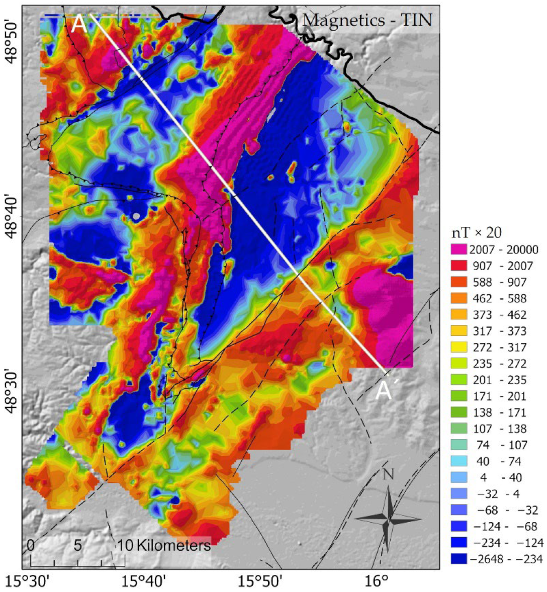
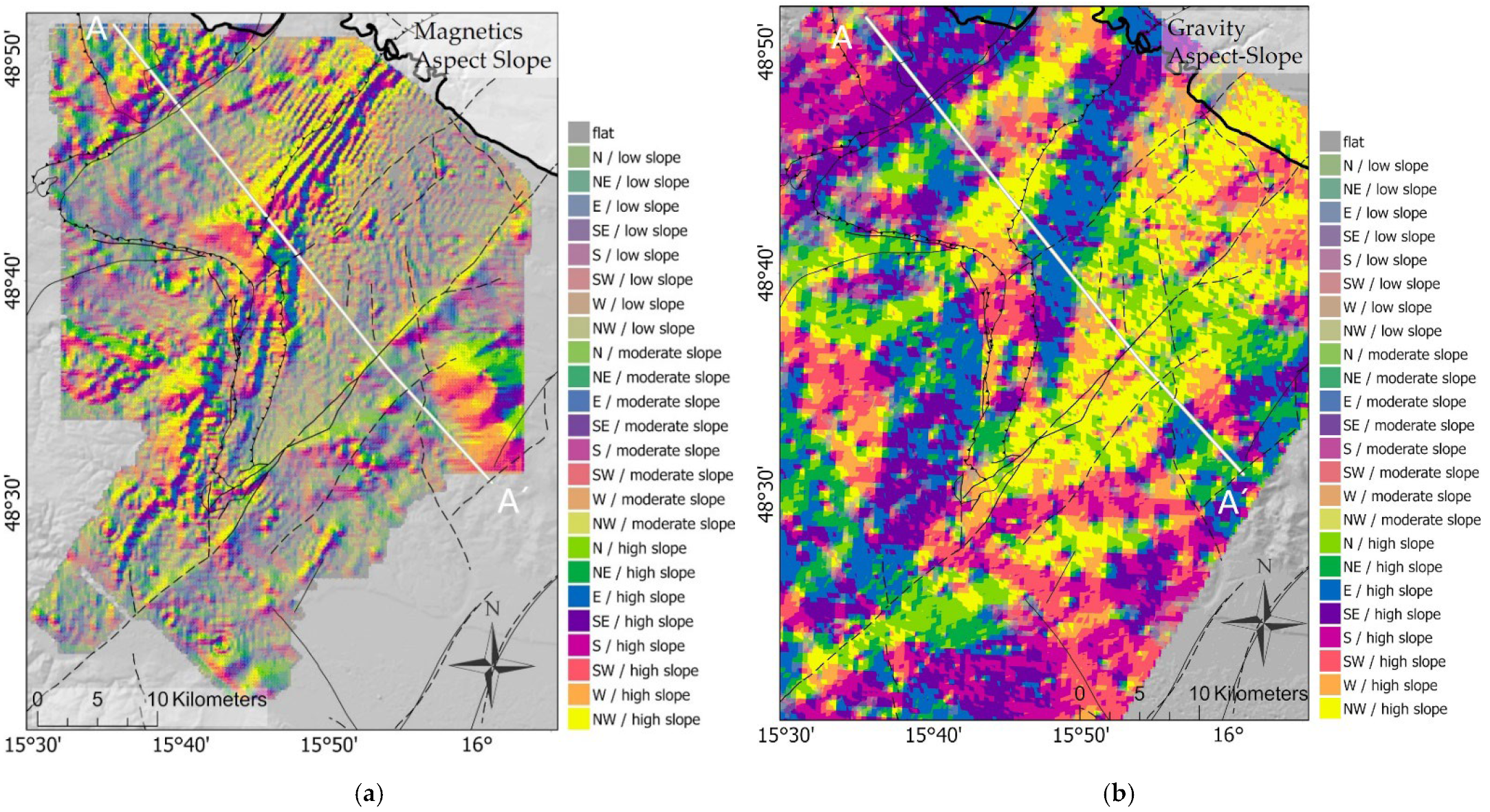
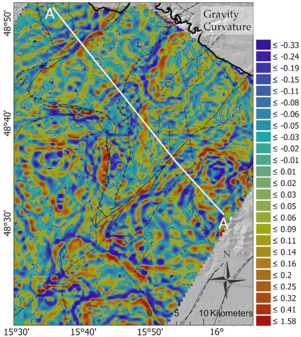
3.1. Fault Lineaments in Map View
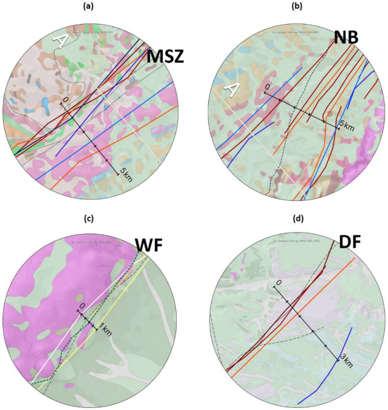
3.2. Comparison along Profile A
4. Discussion
4.1. Comparison of Different Data Sets Using Various GIS Tools
4.2. Location of Profile A
4.3. Map View vs. Profile
4.4. Comparison with Results from Modeling
4.5. Precision of Vintage Aerogeophysical Data
4.6. Experimenting with GIS Tools
4.7. Applicability for Regions with Less or No Geological Information
5. Conclusions
- In general, even if vintage aerogeophysical data lacks today´s accuracy due to less sophisticated technical equipment, they contain valuable information that can be extracted using GIS tools.
- GIS tools prove to be useful for rapid data visualization and interpretation (especially first and second order derivatives and aspect-slope visualization). The comparison of differently transformed fields of various geophysical methods and spatial views can refine the understanding of tectonic structures.
- Lineaments extracted from geophysical data show generally good agreement with the boundaries of geological units and faults. Deep seated and buried sources can be identified by lineaments of magnetic and gravity data and their field transformations—they run mainly parallel to each other. Lineaments identified by methods with shallower investigation depth (AEM and radiometry) can give hints as to whether the geologic structure is buried or not.
- The differences between the positions of lineaments from different methods and datasets can be an indicator for vertical (WF and DF) versus dipping (MSZ and NB) fault geometries.
Supplementary Materials
Author Contributions
Funding
Data Availability Statement
Acknowledgments
Conflicts of Interest
References
- Seiberl, W.; Heinz, H. Aerogeophysikalische Vermessung im Bereich der Kremser Bucht; Technical report BC-2c/83; Geological Survey of Austria: Vienna, Austria, 1986; Available online: http://opac.geologie.ac.at/ais312/dokumente/AeroGeoPh_1986_KremserBucht.pdf (accessed on 27 July 2022).
- Seiberl, W.; Heinz, H. Aerogeophysikalische Vermessung im Raum Ziersdorf; Technical report OC-1d/85; Geological Survey of Austria: Vienna, Austria, 1986; Available online: http://opac.geologie.ac.at/ais312/dokumente/AeroGeoPh_1986_Ziersdorf.pdf (accessed on 27 July 2022).
- Seiberl, W.; Roetzel, R. Aerogeophysikalische Vermessung im Bereich Geras, Niederösterreich; Technical report ÜLG-20/96-97; Geological Survey of Austria: Vienna, Austria, 1998; Available online: http://opac.geologie.ac.at/ais312/dokumente/AeroGeoPh_1998_Geras.pdf (accessed on 27 July 2022).
- Seiberl, W.; Roetzel, R.; Pirkl, H.R. Aerogeophysikalische Vermessung im Bereich von Pulkau/NÖ; Technical report ÜLG-20/94-1; Geological Survey of Austria: Vienna, Austria, 1996; Available online: http://opac.geologie.ac.at/ais312/dokumente/AeroGeoPh_1996_Pulkau.pdf (accessed on 27 July 2022).
- Seiberl, W.; Roetzel, R. Aerogeophysikalische Vermessung im Bereich von Pulkau-Nord/NÖ; Technical report ÜLG-20/95-2; Geological Survey of Austria: Vienna, Austria, 1997; Available online: http://opac.geologie.ac.at/ais312/dokumente/AeroGeoPh_1997_PulkauNordNoe.pdf (accessed on 27 July 2022).
- Meri-Liisa, A. Regional Interpretation of Aerogeophysical Data: Extracting Compositional and Structural Features; Special Paper 39; Geological Survey of Finland: Espoo, Finland, 2005. [Google Scholar]
- Scharbert, H.G. Die Granulite der südlichen Böhmischen Masse. In Geologische Rundschau; Enke: Stuttgart, Germany, 1962; Volume 52, pp. 112–123. [Google Scholar]
- Schermann, O. Über Horizontalseitenverschiebungen arn Ostrand der Böhmischen Masse. Mitt. Ges. Geol. Bergbaustud 1965, 16, 89–103. [Google Scholar]
- Scheidegger, A.E. Untersuchungen des Beanspruchungsplanes im Einflußgebiet der Diendorfer Störung. In Jahrbuch der Geologischen Bundesanstalt; Verlag der Geologischen Bundesanstalt (GBA): Vienna, Austria, 1976; Volume 119, pp. 83–95. [Google Scholar]
- Roštínský, P.; Pospíšil, L.; Švábenský, O. Recent geodynamic and geomorphological analyses of the Diendorf–Čebín Tectonic Zone, Czech Republic. Tectonophysics 2013, 599, 45–66. [Google Scholar] [CrossRef]
- Decker, K. Tektonische Auswertung Integrierter Geologischer, Geophysikalischer, Morphologischer und Strukturgeologischer Daten; Technical report; Geogenes Naturraumpotential Horn-Hollabrunn etc., Projektbericht Bund-Bundesländerkooperation; Geological Survey of Austria: Vienna, Austria, 1999. [Google Scholar]
- Roetzel, R. Bericht 1994–1995 über geologische Aufnahmen im Tertiär und Quartär auf Blatt 22 Hollabrunn mit Bemerkung zur Tektonik am Diendorfer Störungssystem; Report; Geologische Bundesanstalt: Vienna, Austria, 1996. [Google Scholar]
- Figdor, H.; Scheidegger, A.E. Geophysikalische Untersuchungen an der Diendorfer Störung. In Verhandlungen der Geologischen Bundesanstalt; Verlag der Geologischen Bundesanstalt (GBA): Vienna, Austria, 1977; pp. 243–270. [Google Scholar]
- Linner, M.; Reinhard, R.; Benjamin, H.; Hintersberger, E. Two Nappes in the Austrian Part of the Moravian Superunit. In Proceedings of the CETEG 2019: 17th Meeting of the Central European Tectonic Groups, Rozdrojovice, Czech Republic, 24–27 April 2019; Available online: http://opac.geologie.ac.at/ais312/dokumente/Linner_Roetzel_Huet_Hintersberger_2019_Nappes_Austrian_Moravian_Superunit.pdf (accessed on 27 July 2022).
- Schnabel, W.; Fuchs,, G.; Matura, A.; Roetzel, R.; Scharbert, S.; Krenmayr, H.-G.; Egger, J.; Schnabel, W.; Bryda, G.; Mandl, G.W.; et al. Geologische Karte von Niederösterreich (Geological Map of Lower Austria) 1:200.000; Geological Survey of Austria: Vienna, Austria, 2002. [Google Scholar]
- Schnabel, W.; Krenmayr, H.-G.; Mandl, G.W.; Nowotny, A.; Roetzel, R.; Scharbert, S.; Schnabel, W. Geologische Karte von Niederösterreich (Geological map of Lower Austria) 1:200.000, Legende und kurze Erläuterung (Legend and short description). Verlag der GBA: Vienna, Austria, 2002; ISBN 3-85316-017-4. [Google Scholar]
- Supper, R. Auswertung Aerogeophysikalischer Messungen im Bereich Niederösterreich Nord; Internal report; Geological Survey of Austria: Vienna, Austria, 1999. [Google Scholar]
- Baranov, V. A New Method for Interpretation of Aeromagnetic Maps: Pseudo-Gravimetric Anomalies. Geophysics 1957, 22, 359–382. [Google Scholar] [CrossRef]
- Beamish, D. Airborne EM Skin Depths. Geophys. Prospect. 2004, 52, 439–449. [Google Scholar] [CrossRef] [Green Version]
- Dantas, E.L.; Silva, A.M.; Almeida, T.; De Moraes, R.A.V. Old Geophysical Data Applied to Modern Geological Mapping Problems: A Case-Study in the Seridó Belt, NE Brazil. Rev. Bras. De Geociências 2003, 33, 65–72. [Google Scholar] [CrossRef] [Green Version]
- Motschka, K. Gammastrahlenspektroskopie in Österreich. In Geo-Atlas Österreich; Hofmann, T., Schönlaub, H.P., Eds.; Böhlau-Verlag: Vienna, Austria, 2007; pp. 102–103. [Google Scholar]
- Mickus, K. Gravity Method: Environmental and Engineering Applications; Department of Geosciences, Southwest Missouri State University: Springfield, MI, USA, 2003; Available online: https://citeseerx.ist.psu.edu/viewdoc/download?doi=10.1.1.522.2552&rep=rep1&type=pdf (accessed on 27 July 2022).
- Khalaf, A.K.A.; Kordik, P.; Khalil, A.; Mekkawi, M.; El-Bohoty, M.; Rabeh, T.; Refai, M.K.; El-Mahdy, A. Interpretation of Geophysical Data at EL Fayoum—Dahshour Area, Egypt Using Three Dimensional Models. Arab. J. Sci. Eng. 2013, 38, 1769–1784. [Google Scholar] [CrossRef]
- Nabighian, M.N.; Ander, M.E.; Grauch, V.J.S.; Hansen, R.O.; LaFehr, T.R.; Li, Y.; Pearson, W.C.; Peirce, J.W.; Phillips, J.D.; Ruder, M.E. Historical Development of the Gravity Method in Exploration. Geophysics 2005, 70, 63ND–89ND. [Google Scholar] [CrossRef] [Green Version]
- Meurers, B.; Ruess, D. Compilation of a New Bouguer Gravity Data Base in Austria. VGI Osterr. Z. Für Vermess. Und Geoinf. 2007, 2, 90–94. [Google Scholar]
- Meurers, B.; Ruess, D.; Graf, J. A Program System for High Precise Bouguer Gravity Determination. In Proceedings of the 8th International Meeting on Alpine Gravimetry, Leoben, Austria, 4–5 May 2000; pp. 217–226. [Google Scholar]
- Aric, K.; Gutdeutsch, R.; Heinz, H.; Meurers, B.; Seiberl, W.; Adam, A.; Smythe, D. Geophysical Investigations in the Southern Bohemian Massif. Jahrb. Der Geol. Bundesanst. 1997, 140, 9–28. [Google Scholar]
- Kumar, U.; Pal, S.K.; Sahoo, S.D.; Narayan, S.; Mondal, S.; Ganguli, S.S. Lineament Mapping over Sir Creek Offshore and its Surroundings using High Resolution EGM2008 Gravity Data: An Integrated Derivative Approach. J. Geol. Soc. India 2018, 91, 671–678. [Google Scholar] [CrossRef]
- Lobatskaya, R.M.; Strelchenko, I.P. GIS-Based Analysis of Fault Patterns in Urban Areas: A Case Study of Irkutsk City, Russia. Spec. Issue Exhum. Asia 2016, 7, 287–294. [Google Scholar] [CrossRef] [Green Version]
- Pilkington, M.; Tschirhart, V. Practical considerations in the use of edge detectors for geologic mapping using magnetic data. Geophysics 2017, 82, J1–J8. [Google Scholar] [CrossRef]
- Tschirhart, P.; Morris, B. Improved edge detection mapping through stacking and integration: A case study in the Bathurst Mining Camp. Geophys. Prospect. 2015, 63, 283–295. [Google Scholar] [CrossRef]
- Keating, P.; Pilkington, M. An automated method for the interpretation of magnetic vertical-gradient anomalies. Geophysics 1990, 55, 336. [Google Scholar] [CrossRef]
- Miller, H.G.; Singh, V. Potential field tilt—A new concept for location of potential field sources. J. Appl. Geophys. 1994, 32, 213–217. [Google Scholar] [CrossRef]
- Blakely, R.J.; Simpson, R.W. Approximating Edges of Source Bodies from Magnetic or Gravity Anomalies. Geophysics 1986, 51, 1494–1498. [Google Scholar] [CrossRef]
- Raster to TIN. Available online: https://pro.arcgis.com/en/pro-app/latest/tool-reference/3d-analyst/raster-to-tin.htm (accessed on 27 July 2022).
- Slope. Available online: https://pro.arcgis.com/en/pro-app/latest/tool-reference/spatial-analyst/slope.htm (accessed on 27 July 2022).
- Curvature Tool. Available online: https://pro.arcgis.com/en/pro-app/latest/tool-reference/spatial-analyst/curvature.htm (accessed on 27 July 2022).
- Aspect–Slope. Available online: https://pro.arcgis.com/en/pro-app/latest/help/analysis/raster-functions/aspect-slope-function.htm (accessed on 27 July 2022).
- Xie, R.; Xiong, S.; Duan, S.; Wang, J.; Wang, P.; Luo, Y.; Liu, H.; Fan, Z. Noise Estimation in Vector Magnetic Data Derived from Airborne Vector Magnetic System. Geophysics 2020, 85, J71–J83. [Google Scholar] [CrossRef]
- Morris, B.; Leblanc, G.; Prevec, L. An Alternative Simple Procedure to Identify Magnetic and Other Geophysical Anomalies Due to Kimberlite Pipes. In Proceedings of the 2002 SEG Annual Meeting, Salt Lake City, UT, USA, 6–11 October 2002; p. SEG-2002-0712. [Google Scholar]
- Lee, S.; Ross, W.S. 3-D Mitigation of Surface-wave Noise in Spatially Inhomogeneous Media. In Proceedings of the 2008 SEG Annual Meeting, Las Vegas, NV, USA, 9–14 November 2008; p. SEG-2008-2561. [Google Scholar]
- Grauch, V.J.S.; Hudson, M.R. Guides to Understanding the Aeromagnetic Expression of Faults in Sedimentary Basins: Lessons Learned from the Central Rio Grande Rift, New Mexico. Geosphere 2007, 3, 596. [Google Scholar] [CrossRef] [Green Version]
- Brewer, C.A.; Marlow, K.A. Color Representation of Aspect and Slope Simultaneously. In Proceedings of the AutoCarto Conference, Minneapolis, MI, USA, 30 October–1 November 1993; Available online: https://citeseerx.ist.psu.edu/viewdoc/download?doi=10.1.1.453.8620&rep=rep1&type=pdf (accessed on 27 July 2022).
- Roberts, A. Curvature attributes and their application to 3D interpreted horizons. First Break 2001, 19, 85–100. [Google Scholar] [CrossRef]
- Lee, M.; Morris, W.; Leblanc, G.; Harris, J. Curvature analysis to differentiate magnetic sources for geologic mapping’, Geophys. Prospect. 2012, 61, 572–585. [Google Scholar] [CrossRef]
- Cevallos, C.; Kovac, P.; Lowe, S.J. Application of curvatures to airborne gravity gradient data in oil exploration. Geophysics 2013, 78, G81–G88. [Google Scholar] [CrossRef]
- Phillips, J.D.; Hansen, R.O.; Blakely, R.J. The Use of Curvature in Potential-Field Interpretation. Explor. Geophys. 2007, 38, 111–119. [Google Scholar] [CrossRef]
- Florinsky, I. Digital Terrain Analysis in Soil Science and Geology; Academic Press: Cambridge, MA, USA, 2016; p. 486. [Google Scholar]
- Cooper, G.R. Balancing Images of Potential-Field Data. Geophysics 2009, 74, L17–L20. [Google Scholar] [CrossRef]
- Cooper, G.R.J. An Improved Tilt Angle Filter for Potential Field Data. Lead. Edge 2012, 31, 514–517. [Google Scholar] [CrossRef]
- Lee, M.; Morris, W.; Harris, J.; Leblanc, G. An automatic network-extraction algorithm applied to magnetic survey data for the identification and extraction of geologic lineaments. Lead. Edge 2012, 31, 26–31. [Google Scholar] [CrossRef]
- Morris, W.; Ugalde, H.; Kirsch, M.; Gloaguen, R.; Seht, M.; Siemon, B.; Meyer, U. A multi-parameter approach for recognition of anthropogenic noise in aeromagnetic data collected over populated areas: Erzgebirge, Germany. Geophys. Prospect. 2021, 70, 593–617. [Google Scholar] [CrossRef]
- Paoletti, V.; Hintersberger, E.; Schattauer, I.; Milano, M.; Deidda, G.P.; Supper, R. Geophysical Study of the Diendsorf-Boskovice Fault System (Austria). Remote Sens. 2022, 14, 1807. [Google Scholar] [CrossRef]
- Szitkar, F.; Dyment, J. Near-seafloor magnetics reveal tectonic rotation and deep structure at the TAG (Trans-Atlantic Geotraverse) hydrothermal site (Mid-Atlantic Ridge, 26° N). Geology 2015, 43, 87–90. [Google Scholar] [CrossRef]
- Tivey, M.A.; Rona, P.A.; Schouten, H. Reduced crustal magnetization beneath the active sulfide mound, TAG hydrothermal field, Mid-Atlantic Ridge at 26 °N. Earth Planet. Sci. Lett. 1993, 115, 101–115. [Google Scholar] [CrossRef]
- Cooper, G.R.J. An improved terracing algorithm for potential-field data. Geophysics 2020, 85, G109–G113. [Google Scholar] [CrossRef]


| Aerogeohysical Survey/Year | Magnetic Device | Electromagnetic Device/Frequencies | Radiometric Device | Data Per Sec (Mag/EM/Rad) | Average Line Spacing [m] |
|---|---|---|---|---|---|
| Kremser Bucht/1983 | G-801/3 | DIGHEM II/900 Hz (vert./coaxial), 3600 Hz (horiz./coplanar) | GR-800 B | 1/4/1 | 200 |
| Kamptal-Ziersdorf/1983 | G-801/3 | DIGHEM II/900 Hz (vert./coaxial), 3600 Hz (horiz./coplanar) | GR-800 B | 1/4/1 | 200 |
| Pulkau/1994 | Scintrex CS-2 | DIGHEM II/900 Hz (vert./coaxial), 7200 Hz (horiz./coplanar) | Scintrex PGAM-1000 | 10/10/1 | 250 |
| Pulkau north/1995 | Scintrex CS-2 | DIGHEM II/900 Hz (vert./coaxial), 7200 Hz (horiz./coplanar) | Scintrex PGAM-1000 | 10/10/1 | 200 |
| Geras/1996–1997 | Scintrex CS-2 | GEOTECH “Hummingbird”/434 Hz (vertic./coplanar), 3212 Hz (horiz./coaxial), 7002 Hz (vertic./coplanar), 34,133 Hz (horiz./coaxial) | Scintrex PGAM-1000 | 10/10/1 | 200 |
| View | Method | Field under Consideration | Tectonic Structure | Applied Key GIS-Tool | Figure | |||
|---|---|---|---|---|---|---|---|---|
| MSZ | NB | WF | DF | |||||
| Profile A | Gravity | Bougueranomaly (BA) | IDW | Figure 12 | ||||
| Profile Curvature of BA | Profile Curvature | |||||||
| Magnetics | Total Intensity (TI) | IDW | ||||||
| Slope of TI | Slope | |||||||
| Curvature of TI | Profile Curvature | |||||||
| AEM | Apparent Resistivity | IDW | ||||||
| Radiometrics | Uranium | IDW | ||||||
| Potassium | IDW | |||||||
| Thorium | IDW | |||||||
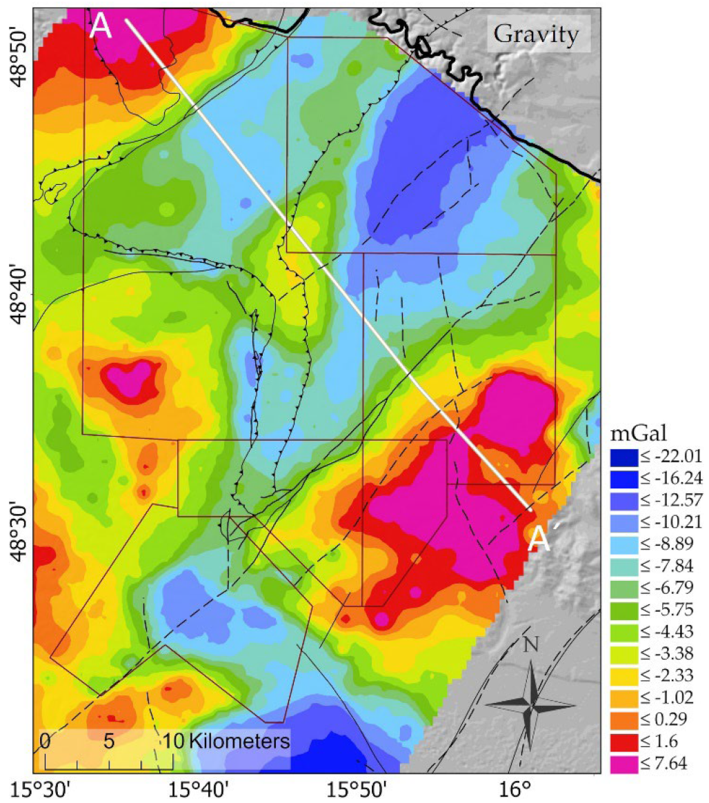
| Map view | Gravity | Bougueranomaly | IDW | Figure 5 | ||||
| Profile Curvature of BA | Profile Curvature | Figure 9 | ||||||
| Aspect Slope of BA | Aspect Slope | Figure 8b | ||||||
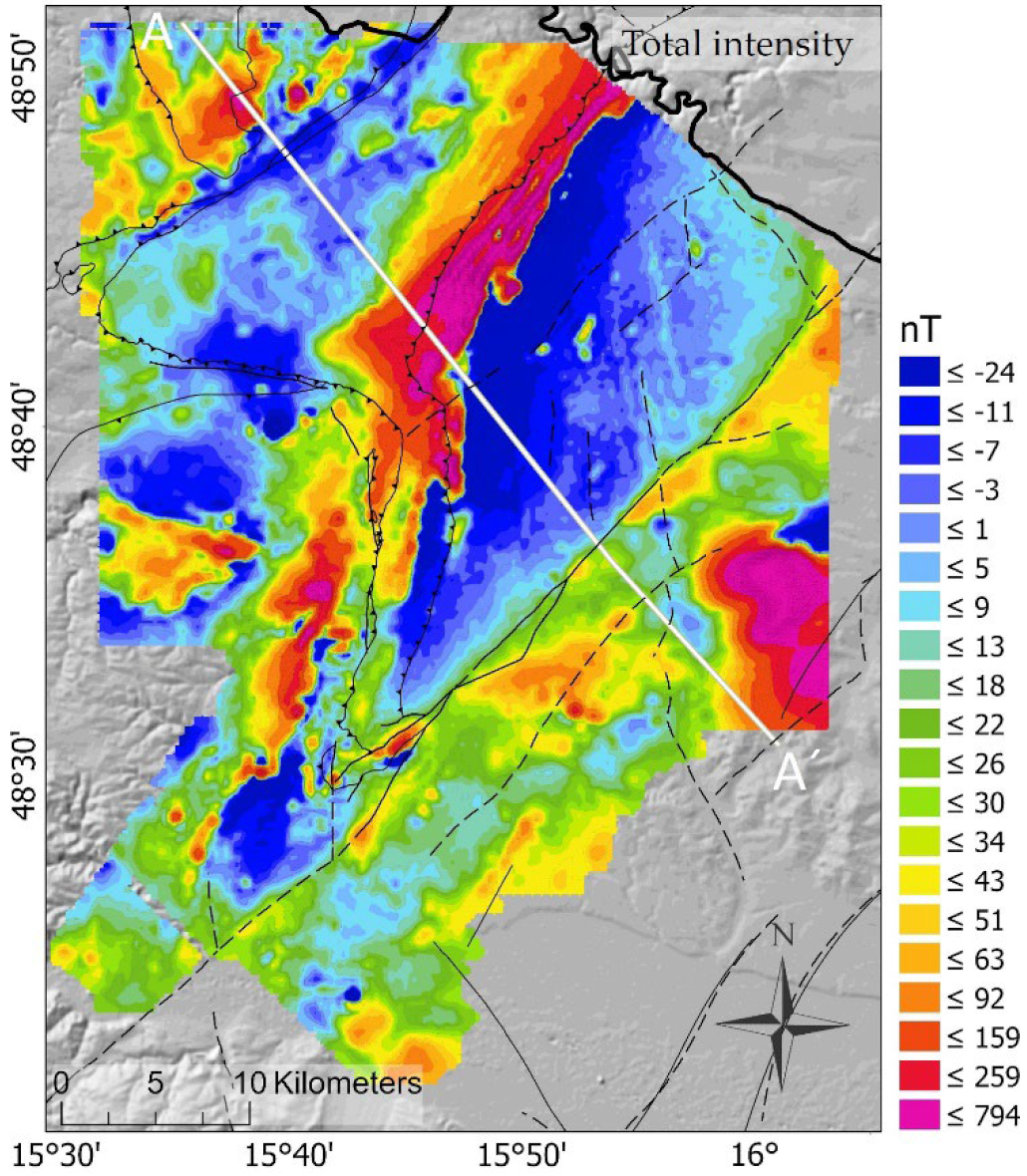
| Magnetics | Total Intensity (TI) | IDW | Figure 2 | |||||
| TI TIN | Raster to TIN | Figure 6 | ||||||
| Slope of TI | Raster to TIN/Slope | Figure 7 | ||||||
| Aspect slope of TI | Aspect Slope | Figure 8a | ||||||
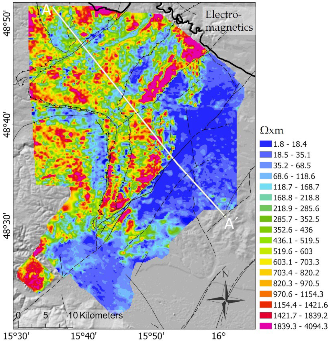
| AEM | Apparent Resistivity | IDW | Figure 3 | |||||
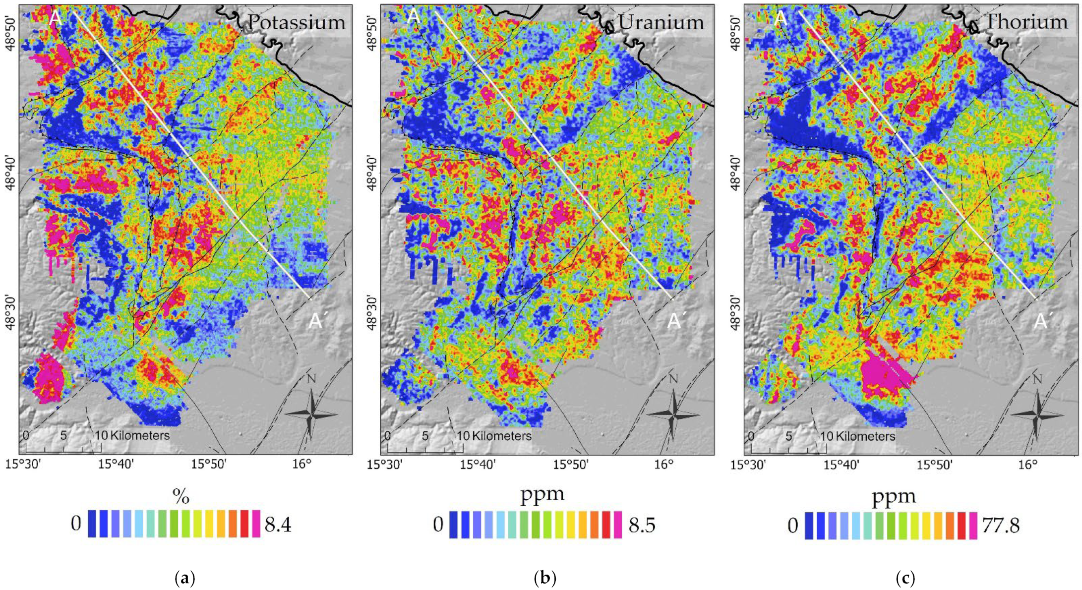
| Radiometrics | Potassium | IDW | Figure 4a | |||||
| Uranium | IDW | Figure 4b | ||||||
| Thorium | IDW | Figure 4c | ||||||
| TIN = triangulated network | visible | |||||||
| Magn. Intensity = Magnetization Intensity [A/m] | visible with limitations | |||||||
| not visible | ||||||||
Publisher’s Note: MDPI stays neutral with regard to jurisdictional claims in published maps and institutional affiliations. |
© 2022 by the authors. Licensee MDPI, Basel, Switzerland. This article is an open access article distributed under the terms and conditions of the Creative Commons Attribution (CC BY) license (https://creativecommons.org/licenses/by/4.0/).
Share and Cite
Schattauer, I.; Hintersberger, E.; Ullrich, C.; Supper, R.; Motschka, K. The Usage of GIS Tools on Vintage Aerogeophysical Data for Simple and Fast Processing with a Focus on Fault Interpretation: An Austrian Case Study. Geosciences 2022, 12, 436. https://doi.org/10.3390/geosciences12120436
Schattauer I, Hintersberger E, Ullrich C, Supper R, Motschka K. The Usage of GIS Tools on Vintage Aerogeophysical Data for Simple and Fast Processing with a Focus on Fault Interpretation: An Austrian Case Study. Geosciences. 2022; 12(12):436. https://doi.org/10.3390/geosciences12120436
Chicago/Turabian StyleSchattauer, Ingrid, Esther Hintersberger, Christian Ullrich, Robert Supper, and Klaus Motschka. 2022. "The Usage of GIS Tools on Vintage Aerogeophysical Data for Simple and Fast Processing with a Focus on Fault Interpretation: An Austrian Case Study" Geosciences 12, no. 12: 436. https://doi.org/10.3390/geosciences12120436