

Deep Electrical Resistivity Tomography for Geophysical Investigations: The State of the Art and Future Directions


1
Institute of Methodologies for Environmental Analysis of CNR, I-85050 Tito, Italy
2
Department of Earth Sciences, University of Ferrara, I-40100 Ferrara, Italy
*
Author to whom correspondence should be addressed.
Geosciences 2022, 12(12), 438; https://doi.org/10.3390/geosciences12120438
Submission received: 28 September 2022
/
Revised: 22 November 2022
/
Accepted: 23 November 2022
/
Published: 28 November 2022
(This article belongs to the Section Geophysics)
Abstract
:Electrical Resistivity Tomography (ERT) is a robust and well-consolidated method largely applied in near-surface geophysics. Nevertheless, the mapping of the spatial resistivity patterns of the subsurface at a depth greater than 1 km was performed in just a few cases by the ERT method, called deep ERT (DERT). Since, in many cases, the term DERT was adopted with ambiguity for geoelectrical explorations varying in depth within a range of 0–500 m, the main goal of this review is to clearly define the DERT method, identifying a threshold value in the investigation depth. The study focuses both on the purely methodological aspects (e.g., geoelectrical data processing in low noise-to-signal ratio conditions; tomographic algorithms for data inversion) and on the technological features (e.g., sensor layouts, multi-array systems), envisaging the future directions of the research activity, especially that based on machine learning, for improving the geoelectrical data processing and interpretation. The results of the more significant papers published on this topic in the last 20 years are analyzed and discussed.
1. Introduction
To date, there has been growing attention paid to novel applications of geophysical tomography for investigating complex geological environments and poorly understood geophysical processes in the shallow part of the Earth’s crust (0–10 km). The exploration of the “Earth Thin Skin” is vital for human life and has an extraordinary social and economic impact (e.g., natural hazards, sustainable geo-energy and geo-resources, climate change and environmental protection, etc.), coherent with the UN Sustainable Development Goals [1].
Electrical and electromagnetic methodologies are currently applied to capture high-resolution 2D, 3D and 4D images of the subsurface resistivity patterns. One of them, Electrical Resistivity Tomography (ERT), is a robust and well-consolidated method for near-surface geophysics, with a wide spectrum of applications in the geological, engineering and environmental sciences. Technological advances (e.g., multi-channel arrays, innovative sensors) and novel tomographic algorithms for data inversion have rapidly transformed ERT into one of the most employed geophysical methods [2].
The first scientific works on the ERT method date back to the period 1990–2000 [3,4,5]. After these pioneer activities, the yearly number of articles focused on this exploration technique published in top-leading journals increased exponentially, testifying the great interest of the scientific community. The ERT method has found an impressive number of applications in near-surface geophysics, from hydrogeology to precision farming, from engineering geology to geohazards, from CO2 storage to the study of the effects of climate change on soil and the subsurface [6,7,8,9,10].
However, most of these applications used the ERT method for investigation depths in the range of 0–200 m (Figure 1), while a very limited number of experimental works have been carried out for exploring deep geological environments (investigation depth greater than 500 m). Information on the electrical properties of the rocks beyond ~1 km depth has been obtained only from direct soundings or passive electromagnetic measurements (e.g., Magnetotelluric—MT) so far. Nevertheless, the MT surveys are strongly affected by anthropic noise in urbanized areas; furthermore, the quality of the MT estimation of the resistivity distribution in the depth range of 0–1 km is quite limited [11], especially if not integrated with other active geophysical techniques. Typically, the MT method is used first as a “pathfinder” role in a large-scale exploration and then, in the shared depth range of investigation, the ERT method can greatly contribute to defining in detail the electrical properties of subsoil. Therefore, it is necessary to improve the efficiency and the capability of the ERT method in deep geological investigations.
The present study reviews the most important scientific results obtained with the ERT method in exploring geological environments with an investigation depth greater than 500 m. Furthermore, a critical analysis of the methodological and technological limits underlying the application of ERT for deep geological investigations is presented and discussed. Finally, the possible and more promising future directions of the research activities about this topic are identified and discussed.
2. Deep ERT Method: Data Processing
When the deep ERT method (DERT) is applied, it is necessary to increase the spacing between the electrodes used for injecting currents into the ground (A and B) and for receiving the voltage signals (M and N). However, this procedure is affected by technical problems due to the use of long electrical cables and the presence of induced currents. For this reason, in the DERT method, the emitting and receiving systems are generally decoupled and the dipole–dipole array configuration is generally adopted. The injecting dipole is physically separated from the receiving one and their mutual distance r is gradually increased along a selected profile on the surface to obtain the 2D resistivity patterns of deep geological environments. Other array configurations can be adopted for obtaining the 3D resistivity models and/or for minimizing the effects of topographic obstacles.
Considering that the amplitude of the voltage signals produced by the emitting sources strongly decreases when the distance r increases (~1/r3 for dipole–dipole array), it is easy to understand that the low signal-to-noise ratio in voltage recordings represents the main problem for the DERT method [12,13]. Furthermore, the presence of conductive zones in the subsurface and of anthropic sources of electromagnetic noise (e.g., pipelines, railway, etc.) on the surface could make this condition worse, reducing the possibility to carry out DERT surveys [13].
For these reasons, the processing and filtering of the noisy voltage recording is the first key action to be approached in any application of the DERT method. The voltage signals recorded during the DERT survey can be modeled as follows:
where s(t) is the useful signal produced by the square wave of a DC current injected into the ground by the emitting dipole and n(t) is the electrical noise. The period of the square wave is generally selected in a range varying from 5 to 60 s. Generally, the noise is due to: (a) a natural component related to the time-dependent changes of the telluric currents induced by the variation of the Earth’s magnetic field; (b) an anthropic component produced by spurious electrical phenomena and man-made activities. To avoid the effects of the electrode polarization, s(t) is a square wave of the DC current with a cyclic inversion of polarity. Previous studies have clearly demonstrated that the geoelectrical noise is not stationary nor Gaussian [14,15].
v(t) = s(t) + n(t)
The amplitude Δs of the useful signal s(t) depends on the intensity of current (I), the apparent resistivity (ϱa) of the investigated subsurface, and the geometry of the electrode array (K):
Δs = (ϱa × I)/K
For the dipole–dipole array configuration:
where a is the spacing of each dipole and n a number for indicating the distance between the electrodes as a multiple of the spacing a. Briefly, the presence of the conductive geological environment, the technological limits for the power intensity of the energizing system and the large distances between the dipoles are the factors that can strongly limit the application of the DERT method.
The main tasks of DERT data acquisition and processing are the following: (i) recordings of the voltage signals with the receiving dipole (MN) in a synchronous mode with the injection of the square wave current by means of the dipole (AB); (ii) removal of the outlier spikes due to the man-made electrical noise and/or technical problems in the electrode contacts; (iii) removal of the long-period drift; and (iv) estimation of the amplitude of the useful signal s(t) [13,14,15].
The first task requires attention to the positioning of the electrodes into the ground to avoid errors in the estimates of the geometrical factor K and perfect synchronization between the emitting and receiving systems with GNSS systems. A DC power generator used to inject currents into the ground with an intensity varying in the range of 5–20A and a set of data loggers able to measure very low-voltage signals (10−3–10−6 Volt) represent the basic hardware for the DERT method. The second task is aimed at controlling the quality of the voltage recordings with a real-time evaluation of the noise level and the use of automatic algorithms for identifying and removing artificial peaks in the voltage signals. The length of the voltage records is modulated on the basis of the noise intensity level [15,16], and this aspect is fundamental to reduce the error in the estimate of the useful signals s(t).
The third task is quite simple and generally approached using the classical polynomial fitting to remove the drift in the voltage recordings [17]. Finally, the last and more relevant task is the estimation of the amplitude of the useful signal s(t) that is generally performed by the stacking, the periodogram, the Fast Fourier Transform (FFT), the Maximum Entropy and the autoregressive model [18,19]. A simplified sequence of the results obtained during the different tasks of the voltage data processing is reported in Figure 2.
Lapenna et al. [15] demonstrated that the most suitable and robust method for evaluating the amplitude of the useful signal Δs is the periodogram technique and the relative error. Since the root-mean-square error associated with the estimate of Δs depends on the variance of the noise and the total number of sampled data (~σ2/N), it strongly decreases with the increase in the time duration of the voltage recordings and, consequently, with the number of samples available for the estimation algorithms [14,15]. Unfortunately, during the field acquisition, a strong increase in the time duration of the energization and voltage data acquisition leads to technical problems, as well as to a relevant increase in the field trip costs. Thus, finding a good compromise between the need to reduce the errors in estimating the amplitude of the useful signals and the duration of the measurement campaigns and cost of field trips, represents a crucial task.
As it concerns the tomographic inversion of the 2D and 3D apparent resistivity values obtained during the field surveys, the published works applied robust and well-consolidated algorithms adopted for the near-surface applications of the ERT method. However, DERT is generally characterized by a low density of data, so that automatic parameterization by near-surface-dedicated software might not be optimal, and adverse effects of regularization might appear in the inversion.
Several inversion methods are well defined in this context, such as the RES2DINV software by Geotomo [3] that is based on the smoothness-constrained least-squares inversion implemented by a quasi-Newton optimization technique, the DCI2D by UBC-GIF [20], which consists of iterative procedures of systems of equations based on objective functions, the BERT software [21], in which the cost function is minimized using a Gauss–Newton scheme, and the ERT-Lab by Multi-Phase Technologies and Geostudi Astier [16], which uses a finite elements (FEM) approach to model the subsoil by adopting a mesh of hexahedrons to correctly incorporate complex terrain topography and is based on a smoothness-constrained least-squares algorithm with Tikhonov model regularization. The only additional critical element is given by the removal of the apparent resistivity values derived from the estimates of the useful signals affected by large errors. Generally, a threshold value of 10% is adopted as the relative error in the estimate of the Δs.
3. Deep ERT Method: Applications
Most of the ERT applications concern near-surface investigations (0–200 m) and are based on the use of the multi-electrode systems and multi-channel cables for data acquisition. The same approach is adopted for investigating electrical resistivity variations with an investigation depth in the range of 200–500 m [22,23,24,25]. The increase in the length of cables and the difficulties of the field acquisition activities that are also time-consuming strongly limit the use of ERT for deeper aims. In fact, to investigate deeper than a 500 m depth threshold, it is necessary to avoid the use of multi-channel cables, to adopt decoupled energizing and measuring systems and to apply advanced approaches for data acquisition and analysis, representing surely a challenging task. Thus, in this section, we review the most relevant works focused on the application of the 2D and 3D DERT method based on the use of decoupled transmitting and receiving systems, for investigation depths greater than 500. It is remarkable to highlight that few papers have been published on this topic in the last 20 years, and only in recent years have novel applications of this method been made available.
One of the first applications of deep electrical imaging was carried out for studying the Ahuachapan–Chipilapa geothermal field (El Salvador) [26]. A total of four resistivity profiles with a maximum length of 10 km were obtained with a dipole–dipole array configuration. In total, two different dipole spacings of 500 m and 1000 m were used, and the measurements were performed using a 35 KW power generator for injecting a square-wave current into the ground. The results of the 2D resistivity images helped to reconstruct the geometry of conductive zones associated with the presence of geothermal fluids and supported the interpretation of the magnetotelluric soundings carried out in the same area.
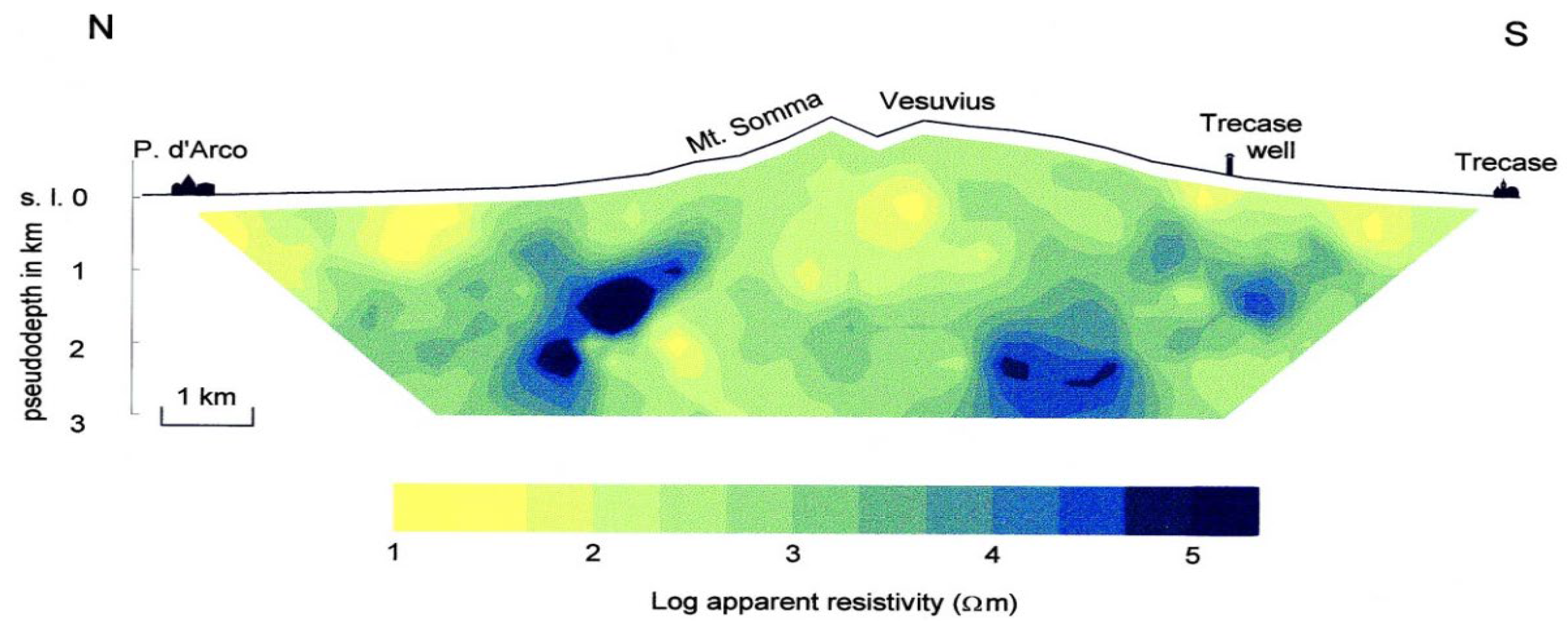
Another pioneering work was planned for investigating the volcanic structure of Mt. Vesuvius (Italy) [27], which is considered the most dangerous volcano in the world. An apparent resistivity pseudosection was carried out across the N–S profile of Vesuvius; the length of the profile was 13 km, and the basic electrode spacing about 500 m.
The 2D pseudosection resistivity profile is reported in Figure 3, where a pseudodepth of about 3 km was depicted. The limit of this application is the absence of a tomographic inversion procedure. However, the general apparent resistivity pattern defined a roughly horizontal alternation of conductive and resistive bodies within the investigated depth range. The main geoelectrical result highlighted the largely extended, relatively low resistivity zone in the central part of the profile, closely in correspondence to the Somma caldera, including, in the middle, the top terminal part of Vesuvius. Finally, these results were compared and integrated with Self Potential (SP) and MT ones to investigate the shallow and deep regions of the volcanic area.
Another one of the pioneering activities that used the DERT method concerned a study performed close to the site of the German Continental Deep Drilling Project (KTB). Storz et al., 2000 [28] carried out a 2D ERT profile using 44 dipoles; they adapted the classical ERT array configuration using separate injecting and receiving dipoles (Figure 4). The length of the profile was 22 km, the electrode distance was 500 m, the maximum amplitude of the injected current was 15 A and the square wave period of the current injected into the ground was 20 s. The temporal duration of the registrations was a maximum of 25 min.
The data processing of 968 voltage recordings was carried out using the classical flowchart based on the drift potential corrections, recursive notch filtering and outliers’ removal, band-pass filtering and stacking. Due to the low signal-to-noise ratio of the voltage recordings and the choice to accept only useful signals affected by a limited error (smaller than 10%), more than 50% of the voltage recordings was eliminated. Finally, the apparent resistivity values were calculated and inverted for obtaining a 2D resistivity image of the subsurface. A simultaneous iterative reconstruction technique (SIRT) was adopted; it is based on the discretization of the subsurface into N grid elements, where the cells are small compared to the dipole spacing [29]. The maximum investigation depth reached during this first test of deep ERT was about 4 km (Figure 5).
The interpretation of the resistivity image was well correlated with other geophysical models, with the results of downhole logging in the KTB drillholes and with resistivity measurements on core geological sounding [30,31]. The spatial resistivity distribution was able to reconstruct the extension of the conductive structures (ρ < 10 Ωm) with a steep inclination related to the presence of faults. In these highly fractured zones, there is the presence of permeable material and fluid circulation. The rapid increase in the resistivity values (ρ > 3000 Ωm) at depths between 2 and 3 km was associated with the presence of the Falkenberg Granite Massif.
This work can be considered the first experimental test of the DERT method with an investigation depth of 4 km; however the spatial resolution of the resistivity pattern was strongly limited by few apparent resistivity values obtained for the large spacings of the dipole–dipole array system.
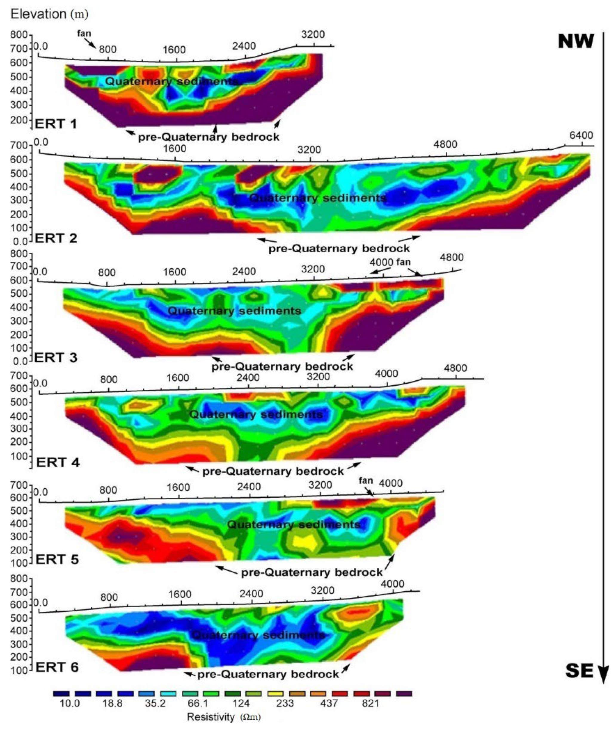
Colella et al., 2004 [32] applied the DERT method for obtaining the first high-resolution resistivity imaging of the High Agri Valley basin (southern Italy), representing one of the more complex components of the Quaternary fault network of the Apennine chain. During the field campaigns, six 2D DERT profiles perpendicularly oriented to the longitudinal basin direction were carried out using the dipole–dipole array configuration. The spacing of dipoles was 200 m, the maximum distance between emitting and receiving dipoles was n times the basic electrode spacing, with a mean investigation depth of about 500 m. The lengths of the profiles were in the range of 4–7 km. Algorithms for detrending and filtering voltage recordings and the FFT method were used for extracting the useful voltage signals. The high resolution of the electrical images delineated the complex geometry of the High Agri Valley basin (Figure 6).
A comparison between the results of the 2D DERT profiles and some seismic reflection profiles carried out in the same area confirmed the high spatial resolution of the DERT. The electrical imaging highlights the irregular shape of the basin, which is bordered by shallow faults and filled with Pleistocene alluvial deposits.
In the longitudinal cross-section, the basin appears as a mosaic of fault-bounded blocks forming three different depocenters separated by intrabasinal highs. In the transverse cross-section, the basin is an irregular graben, locally asymmetric to the northeast, and with secondary grabens due to antithetic faults. The geophysical study of the High Agri Valley basin has been improved with new DERT field measurements [33]. One of them is 27 km long with an electrode distance of about 400 m. The papers describe the new acquisition system composed of a multi-electrode and a multichannel automatic system with 12 channels. To date, a 3D resistivity model of the basin is available [16].
The same methodological approach was adopted in other interesting studies concerning the investigation of geothermal areas and groundwater aquifer in a karst environment located in the southern Apennine chain (Italy) [34,35].
Balasco et al. [36] applied the DERT and the MT methods to investigate the Aterno Valley (central Italy) that was struck by the 2009 L’Aquila earthquake. The integration of these two different methods allowed the authors to increase the spatial resolution of the subsurface resistivity images. The MT method is suitable for investigating deep geological structures in a depth range of 0–10 km, but it is characterized by low spatial resolution in shallow subsurface investigations. Therefore, using the DERT method in the common depth range of investigation (01.2 km), a resistivity model with a high resolution could be obtained, suggesting that integrating DERT with MT seems to optimize the spatial resolution of the resistivity subsurface pattern at different investigation depths.
The length of the DERT profile was 8 km, the electrode spacing was 400 m and the maximum distance between the injecting and receiving systems was eight times the electrode spacing. The measurements were performed with a dipole–dipole array configuration. The system consisted of a transmitting station, which injected a square-wave current, with a maximum energizing current of 5A, into the ground and a multichannel receiver system composed of four remotely multichannel dataloggers controlled by a laptop. For each current injection, eight voltage recordings lasting from 5 to 20 min were simultaneously acquired. A total of 112 voltage recordings, related to the different position of the electrodes along the profile, were collected. The data processing was carried out using the classical stacking and FFT methods.
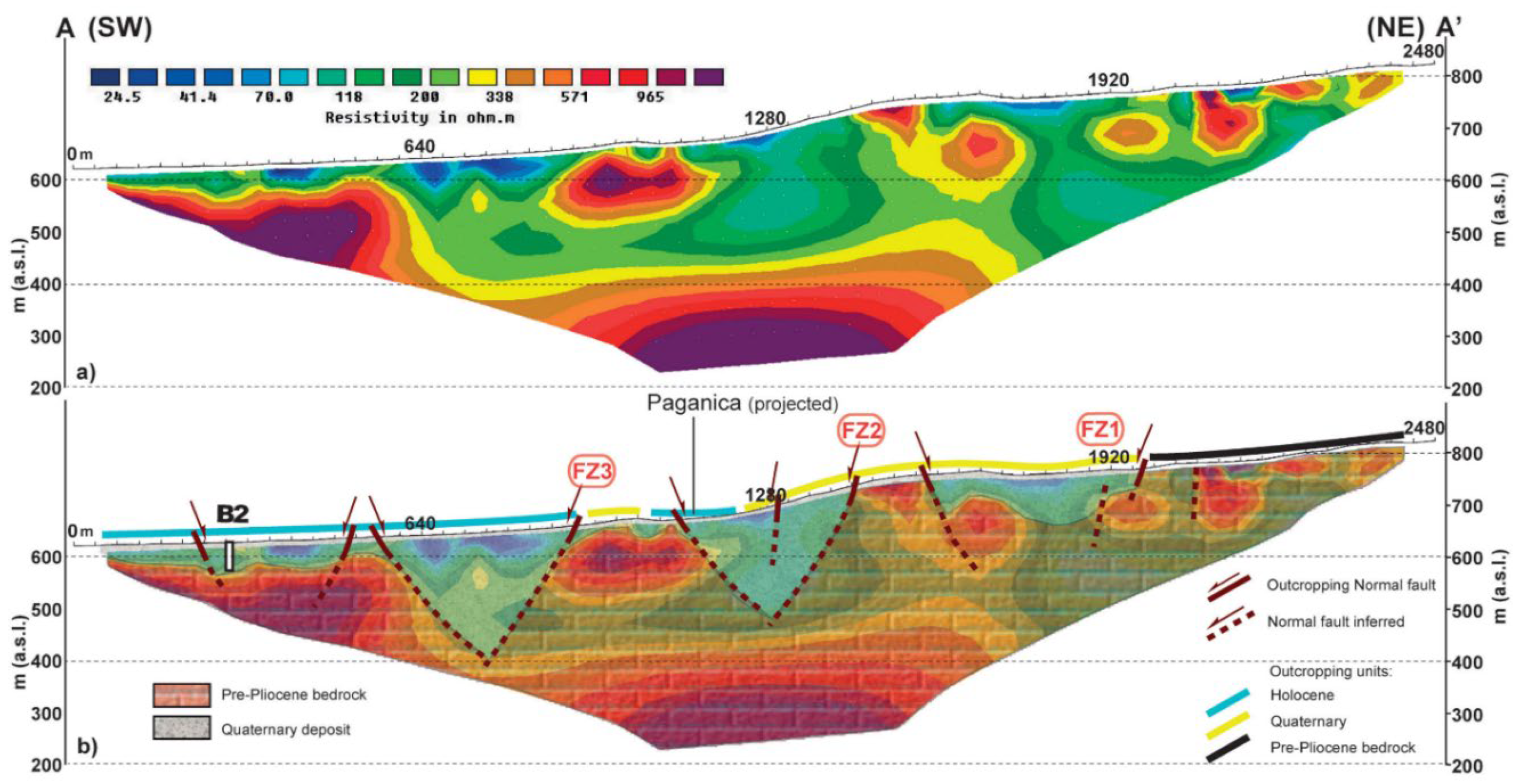
The apparent resistivity values were inverted by means of the inversion algorithm DCIP2D [20,37]. Figure 7 shows the resistivity tomographic image that is characterized by resistivity values varying from 10 Ωm to over 2500 Ωm and many lateral discontinuities related to many regional faults, both thrusts and successive extensional features. To the end of the DERT profile, several highly resistive (ρ > 1000 Ωm) zones, separated by relative conductive (200–500 Ωm) areas, are observed, testifying a complex tectonic-stratigraphical structure. At about 7000 m along the DERT profile, the sharp vertical resistivity contrast highlights the Paganica Fault.
In this area of Central Italy, Pucci et al. [38] studied and improved the knowledge of the complex geometry of the Paganica–San Demetrio basin using the DERT method. They carried out the 2D DERT measurements along three different profiles perpendicularly oriented to the eastern edge of the Quaternary basin and the Paganica fault (Figure 8).
A multi-electrode 2D device by means of the ABEM Terrameter SAS-4000 instrument connected to ABEM ES1064 C multiplexer was adopted for the field data acquisition. They used a 2.52 km long cable, with a set of 64 stainless steel electrodes and offset of 40 m, and a roll-along scheme for data acquisition with Wenner-alpha and pole-dipole array configurations. The length of the three profiles was, respectively, 2.52 km, 6.38 km and 3.8 km.
They processed apparent resistivity data using the X2IPI software for data filtering, while data inversion was carried out with RES2DINV software [2]. The interpretation of the 2D resistivity models with geological constraints contributed to better describing the shape of the basin. The results suggested a southeastward deepening of the Paganica–San Demetrio Basin from ∼200–300 m to the maximum depocenter of ∼600 m, largely exceeding the known thickness of the continental sequence. Complex lateral and vertical heterogeneous resistivity regions suggested the existence of several tectonic features that displaced the original Meso-Cenozoic multilayer producing buried cumulative landforms and controlling the development of depressions, later filled with sequences of Plio-Quaternary continental deposits. The geological interpretation of the tomographic images showed a structural style consisting of SW dipping, leading normal faults from which NE dipping, antithetic faults splay out, defining grabens acting as sedimentary traps.
Carrier et al. [39] adopted, for the first time, the new Fullwaver instrument of the Iris company for exploring the geothermal field in the Greater Geneva Basin (Switzerland). A 2D DERT profile with a length of 4.8 km and an investigation depth of about 1 km was planned in an urbanized area affected by electrical noise.
The new system consists of 25 V Fullwaver nodes for receiving voltage signals and 1I Fullwaver nodes for the injection of the current with reverse polarity into the subsurface with a maximum intensity of 10 A. For each receiving node, a set of three aligned electrodes with spacing of 50 m is installed. This new system is extremely user-friendly and can be easily adopted for DERT surveys in urban areas. Furthermore, the system does not require long cables and any fixed array configurations, 2D and 3D DERT surveys can be carried out without any geometrical constraints. During the field surveys, a set of 2318 voltage recordings was obtained; a post-processing and a quality control of the data were carried out using the PROSYS software and ERT-Lab [40]. After this step, a total of 1746 useful voltage signals were selected and used for estimating the apparent resistivity values. Finally, the BERT algorithm [37] allowed the authors to obtain the 2D resistivity model (Figure 9).
The result of the 2D DERT highlights a high-resistivity zone in the SE part of the profile and at a depth between 250 m and 650 m. In the central part of the DERT profile, the low resistivity values are related to the presence of groundwater, while the low resistivity values at greater depths crosscut the Upper Cretaceous–Lower Cenozoic limits. For this study, the good agreement between the results obtained with the DERT method with other more robust and consolidated geophysical methods, the gravity and seismic exploration methods, is remarkable.
Lajaunie et al. [41] applied the deep ERT method for investigating the Sèchilienne slope, which is one of the largest and most active landslides in the European Alps (France). The geological and hydrogeological settings of this complex landslide were largely studied with different geophysical methods, but the surveys produced only 1D and 2D images of the subsurface. This work represents one of the first applications of the deep 3D ERT method to investigate a landslide area. They obtained a 3D resistivity model of the Sèchilienne slope up to a depth of 500 m.
The geophysical field campaign was carried out using a FullWaver system made of 23 V receiving nodes with two orthogonal MN dipoles with spacing of 50 m and a 1 I energizing node with a fixed electrode and a moving electrode B along 30 selected points within the landslide area. The PROSYS and the BERT software were used for the voltage data processing and the resistivity data inversion, respectively (Figure 10).
The 3D model is characterized by two different resistivity anomalies. An anomaly with high resistivity values was identified in the western sector of the model and associated with very fractured and dry material. The absence of the water sources in this area confirms the high permeability of the slope material. At the surface, the high resistivity values seem to be aligned with the major faults. The conductive-zone anomaly at the east of the landslide (Sabot fault) was detected and interpreted as a perched aquifer. On the basis of geological and hydrogeological studies, the unstable zones are correspond with the resistive anomaly. Notwithstanding the poor spatial resolution of the resistivity measurements, the results contributed to better describing the hydrogeological setting of the investigated area.
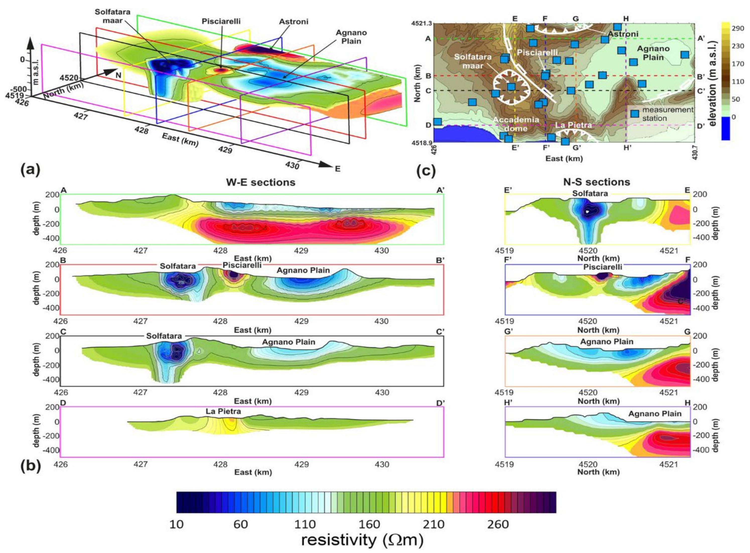
Troiano et al. [42] studied the complex geometry of the central sector of the Campi Flegrei caldera (Italy), applying a deep 3D ERT tomographic approach. They adopted the new Iris FullWaver instrument system consisting of 12 dual-channel receivers with a sampling rate of 10 ms and an Iris VIP 10,000 electrical transmitter for injecting DC current into the ground, with a change of polarity every 2 s. In a selected area of the Campi Flegrei caldera, the field measurements were carried out with a dense spatial distribution of receiving stations; for each point, two dipoles with a spacing of 100 m perpendicularly oriented were installed. The scholars adopted the principal component decomposition method to remove the electrical noise and extracting the useful voltage signals.
The inversion of the apparent resistivity values was carried out using the commercial software ERTlab3D, and a 3D resistivity imaging of the investigated area was obtained (Figure 11). The maximum investigation depth was about 400 m, which was evaluated using a robust and quantitative method for evaluating the depth of investigation.
The 3D resistivity model of the investigated area clearly identifies two very conductive zones: the Solfatara maar and the Agnano Plain. The high resolution of the tomographic image allowed the authors to reconstruct the geometry of these structures. Furthermore, a resistive zone is clearly visible with a conical shape that is associated with the Pisciarelli fumarole. The quality of the results confirms the capacity of deep ERT to contribute to describing the geometry of geological structures in active volcanic areas.
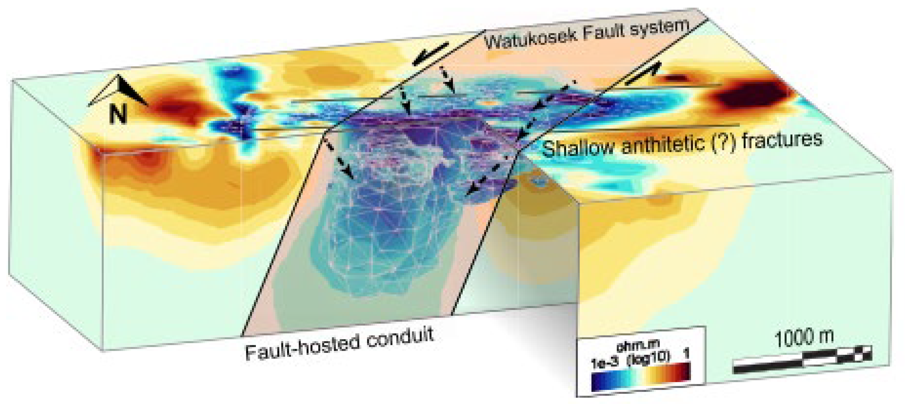
Mazzini et al. [43] applied the deep ERT method for studying an interesting volcanic area located in the East Java Basin representing the largest eruptive clastic system on Earth. The geoelectrical survey was planned for investigating the Lusi eruptive site, where a geothermal system was pierced onto the surface along the Watukosek fault system in May 2006.
During the field campaigns, the Fullwaver system of the IRIS company was used for carrying out 3D deep ERT in an area of 15 km2. The main characteristics and performances of the hardware and the software of this system were already described in the previous paragraphs. A set of 25 V Fullwaver receiving nodes and 1 I Fullwaver energizing nodes was used for obtaining 3596 values of the useful voltage signals. After the pre-processing and filtering procedures to remove the voltage recordings with a very low signal-to-noise ratio, a set of 2331 values was selected to perform the inversion with the BERT software.
The main results of the 3D ERT opened the way for investigating the possible correlation between the presence of the Watukosek fault system, the movements of the deep fluids and the formation of the Lusi geothermal system (Figure 12). Furthermore, the results have great implications for supporting the local authorities in planning and managing hazard mitigation activity.
Rizzo et al. [44] carried out an innovative experiment with the 3D deep ERT method for exploring the Larderello geothermal area (Italy), the oldest geothermal field in the world under exploitation for power production. For the first time, a 3D Surface-Hole Deep Electrical Resistivity Tomography (SH-DERT) was designed and carried out for studying a complex geothermal field and operating in extreme environmental conditions.
The injecting and receiving systems were distributed on a surface with an extension of 6 km2 and in the Venelle-2 well with a depth of 1.6 km. A log cable with the capacity to operate at high temperatures was used to manage and control 12 cylindrical steel electrodes with a diameter of 20 mm and a length of 1.5 m. All the measurements were carried out by means of a multi-channel datalogger synchronized with the injecting systems (square-wave of DC current with a maximum intensity of 10 A and polarity inversion of 32 s). A dipole–dipole array configuration was adopted with a maximum distance between injecting and receiving dipoles of 1.600 m.
The data processing of the voltage signals recorded during the field surveys was performed with classical methods (detrending, filtering and FFT technique). A total of 10% of the data collected was removed due to the very low signal-to-noise ratio. To perform the resistivity data inversion, the authors applied the ERT-Lab software. In a first step, they inverted only the apparent resistivity data estimated with data coming from dipoles installed on the surface; in a second step, they used all data available, including the apparent resistivities calculated using the sensors in the borehole too (Figure 13). The investigation depth of the surface 3D DERT was about 800 m, while the 3D SH-DERT was 1600 m. A shallow conductive nucleus (ϱ < 10 Ωm) bound by zones with relatively high resistivity zones is clearly identified. The DERT measurements carried out with electrodes in the borehole and on the surface strongly increase the spatial resolution of the 3D resistivity pattern and are of great interest for the scientific community involved in the study of geothermal fields.
4. Discussion
To date, the application of the DERT method still remains limited to a few case studies with an investigation depth greater than 500 m. The main characteristics of the DERT applications discussed in the previous paragraph are summarized in Table 1.
However, in the last five years, this topic raised important attention in the scientific community, with an increase in interesting and challenging works. The main applications concern the investigation of the complex geometry of the seismically active structures, the mapping of fluids and gases in volcanic zones and the exploration of the geothermal fields for energy production. Moreover, in these recent papers, technological advances permitted an increase in the maximum investigation depth. For this reason, we can define a survey carried out with an exploration depth of at least 500 m as deep ERT (DERT) investigation.
As it concerns the field survey, distributed and high-spatial-density sensor networks of measuring and energizing dipoles are generally adopted. The measuring dipoles are equipped with instruments to record low-voltage signals (10−3–10−6 V), while a mobile system equipped with a high-electrical-power generator is used for the injection of the current square wave (max 20 A) into subsoil with the polarity regularly inverted. The frequency of these inversions is extremely low, and the approximation of the direct electrical current (f = 0) is acceptable. Furthermore, there is great attention paid to the sensors realized with materials to ensure an optimal contact between electrodes and hosting to reduce the anthropic noise, especially when they are installed in boreholes. All the sensors for measuring electrical potential are remotely controlled by means of a multi-channel datalogger.
As it concerns methodological advances, tomographic inversion is carried out with robust and well-assessed algorithms used for the application of the ERT method in near-surface investigations. Recently, there has been a growing interest in open-source software based on Python tools and extraordinary opportunities related to the use of high-performance computing facilities. Then, there are no limits or critical problems in applying the large spectrum of commercial and open-sources software already available for DERT data inversion.
In this scenario, a critical aspect is the absence of innovative algorithms for the data processing and filtering of the voltage recordings with a low signal-to-noise ratio. They are generally based on standard statistical and spectral decomposition techniques, as well as detrending, outlier removal and Fourier analysis for evaluating the amplitude of the useful voltage signals.
One of the most promising future directions of research on the DERT method could be represented by the application of Machine Learning algorithms for noise removal and signal identification in the voltage recordings [45,46,47,48]. The novel distributed sensors that are remotely controlled can acquire a long time series of voltage measurements, and this large amount of data could be easily processed with Machine Learning algorithms.
Another promising research activity could be based on the application of advanced statistical approaches for better characterizing the inner dynamical structure of the electrical noise that is generally assumed to be Gaussian, although it is widely recognized that this assumption is too simple for many geophysical signals [49,50,51].
5. Conclusions
In this work, a critical analysis of the main advantages and limitations concerning the applications of the deep ERT method is presented and discussed.
The main technological advances are related to the use of a dense network of receiving and injecting dipoles that can easily installed on the surface and in boreholes without any geometrical limitations. The dipoles are decoupled and separately distributed, so that the connection with long cables is not necessary. Furthermore, a new class of power generators for injecting DC currents into the ground with a maximum intensity of 20A is available. These technological advances make it possible to increase the distance between emitting and receiving systems and, consequently, to investigate the resistivity pattern of the subsurface at greater depths.
The main limitation of the DERT method is related to the degradation of the quality of voltage recordings when the distance between the dipoles increases. The amplitude of the useful voltage signals generated by the current strongly decrease (~1/r3) and it becomes gradually contaminated by the electrical noise; the extreme low signal-to-noise ratio makes an accurate estimate of the useful signal impossible.
To reduce the errors associated with the extraction of the useful signals from the voltage time series and, as a consequence, to obtain apparent resistivity values for deep layers, it is mandatory to adopt advanced statistical and mathematical tools. One of the most promising research directions is the introduction of algorithms based on Artificial Intelligence and Machine Learning methods that could strongly improve the ability to process large numbers of voltage recordings.
Finally, an improvement of the DERT investigation depth (>1 km) could open the way for a more relevant contribution for studying a wide class of challenging geological problems (e.g., monitoring CO2 storage, migration of deep gases and fluids in volcanic areas, evaluation of the ice thickness in polar regions).
Author Contributions
Conceptualization, M.B.; V.L.; E.R.; L.T.; methodology, M.B.; V.L.; E.R.; L.T.; writing—original draft preparation, M.B.; V.L.; E.R.; L.T.; supervision and project administration, V.L. All authors have read and agreed to the published version of the manuscript.
Funding
This research received no external funding.
Conflicts of Interest
The authors declare no conflict of interest.
References
- Capello, M.A.; Shaughnessy, A.; Caslin, E. The Geophysical Sustainability Atlas: Mapping geophysics to the UN Sustainable Development Goals. Lead. Edge 2021, 40, 1. [Google Scholar] [CrossRef]
- Loke, M.H.; Chambers, J.E.; Rucker, D.F.; Kuras, O.; Wilkinson, P.B. Recent developments in the direct-current geoelectrical imaging method. J. Appl. Geophys. 2013, 95, 135–156. [Google Scholar] [CrossRef]
- Loke, M.H.; Barker, R.D. Rapid least-squares inversion of apparent resistivity pseudosections using a quasi-Newton method. Geophys. Prospect. 1996, 44, 131–152. [Google Scholar] [CrossRef]
- Loke, M.H.; Barker, R.D. Practical techniques for 3D resistivity surveys and data inversion. Geophys. Prospect. 1996, 44, 499–523. [Google Scholar] [CrossRef]
- Binley, A.; Henry-Poulter, S.; Shaw, B. Examination of solute transport in an undisturbed soil column using electrical resistance tomography. Water Resour. Res. 1996, 32, 763–769. [Google Scholar] [CrossRef]
- Perrone, A.; Lapenna, V.; Piscitelli, S. Electrical resistivity tomography technique for landslide investigation: A review. Earth Sci. Rev. 2014, 135, 65–82. [Google Scholar] [CrossRef]
- Bellanova, J.; Calamita, G.; Giocoli, A.; Luongo, G.; Macchiato, M.; Perrone, A.; Uhlemann, S.; Piscitelli, S. Electrical resistivity imaging for the characterization of the Montaguto landslide (southern Italy). Eng. Geol. 2018, 243, 272–281. [Google Scholar] [CrossRef] [Green Version]
- Finizola, A.; Revil, A.; Rizzo, E.; Piscitelli, S.; Ricci, J.; Morin, B.; Angeletti, L.; Mocochain, L.; Sortino, F. Hydrgeological insights at Stromboli volcano (Italy) from geoelectrical, temperature, and CO2 soil degassing investigations. Geophys. Res. Lett. 2006, 33, L17304. [Google Scholar] [CrossRef] [Green Version]
- Bergmann, P.; Schmidt-Hattenberger, C.; Labitzke, T.; Wagner, F.M.; Just, A.; Flechsig, C.; Rippe, D. Fluid injection monitoring using electrical resistivity tomography five years of CO2 injection at Ketzin, Germany. Geophys. Prospect. 2017, 65, 859–875. [Google Scholar] [CrossRef]
- Oldenborger, G.A.; LeBlanc, A.M. Monitoring changes in unfrozen water content with electrical resistivity surveys in cold continuous permafrost. Geophys. J. Int. 2018, 215, 2. [Google Scholar] [CrossRef]
- Zhdanov, M. Geophysical Electromagnetic Theory and Methods, 1st ed.; Elsevier: Amsterdam, The Netherlands, 2009; ISBN 9780444529633. [Google Scholar]
- Alfano, L. Dipole-dipole deep geoelectrical soundings over geological structures. Geophys. Prospect. 1980, 28, 283–296. [Google Scholar] [CrossRef]
- Lapenna, V.; Satriano, C.; Patella, D. On the methods of evaluation of apparent resistivity under conditions of low message-to-noise. Geothermics 1987, 16, 487–504. [Google Scholar] [CrossRef]
- Cuomo, V.; Lapenna, V.; Macchiato, M.; Patella, D.; Satriano, C.; Serio, C. Statistical analysis of stationary noisy voltage recordings in geoelectrics. Boll. Geofis. Teor. Appl. 1990, 24, 205–210. [Google Scholar]
- Lapenna, V.; Macchiato, M.; Patella, D.; Satriano, C.; Serio, C.; Tramutoli, V. Statistical analysis of non-stationary voltage recordings in geoelectrical prospecting. Geophys. Prospect. 1994, 42, 917–952. [Google Scholar] [CrossRef]
- Rizzo, E.; Giampaolo, V. New Deep Electrical Resistivity Tomography in the High Agri Valley Basin (Basilicata, Southern Italy). Geomat. Nat. Hazards Risk 2019, 10, 197–218. [Google Scholar] [CrossRef] [Green Version]
- Bendat, J.S.; Piersol, A.G. Random Data: Analysis and Measurements Procedures; John Wiley & Sons: New York, NY, USA, 1986. [Google Scholar]
- Box, G.E.P.; Jenkins, G.M. Time Series Analysis Forecasting and Control; Holden Day: San Francisco, CA, USA, 1976. [Google Scholar]
- Jenkins, G.M.; Watts, D.G. Spectral Analysis and Its Applications; Holden Day: San Francisco, CA, USA, 1968. [Google Scholar]
- Oldenburg, D.W.; Mcgillivray, P.R.; Ellis, R.G. Generalized subspace method for large scale inverse problems. Geophys. J. Int. 1993, 114, 12–20. [Google Scholar] [CrossRef] [Green Version]
- Rucker, C. Advanced Electrical Resistivity Modelling and Inversion Using Unstructured Discretization. Ph.D. Thesis, University of Leipzig, Leipzig, Germany, 2010. [Google Scholar]
- Goebel, M.; Pidlisecky, A.; Knight, R. Resistivity imaging reveals complex pattern of saltwater intrusion along Monterey coast. J. Hydrol. 2017, 551, 746–755. [Google Scholar] [CrossRef]
- Legaz, A.; Vandemeulebrouck, J.; Revil, A.; Kemna, A.; Hurst, A.W.; Reeves, R.; Papasin, R. A case study of re-sistivity and self-potential signatures of hydrothermal instabilities, Inferno Crater Lake, Waimangu, New Zealand. Geophys. Res. Lett. 2009, 36, L12306. [Google Scholar] [CrossRef]
- Lévy, L.; Maurya, P.K.; Byrdina, S.; Vandemeulebrouck, J.; Sigmundsson, F.; Árnason, K.; Ricci, T.; Deldicque, D.; Roger, M.; Gilbert, B.; et al. Electrical resistivity tomography and time-domain induced polarization field investigations of geothermal areas at Krafla, Iceland: Comparison to borehole and laboratory frequency-domain electrical observations. Geophys. J. Int. 2019, 218, 1469–1489. [Google Scholar] [CrossRef] [Green Version]
- Revil, A.; Finizola, A.; Piscitelli, S.; Rizzo, E.; Ricci, T.; Crespy, A.; Angeletti, B.; Balasco, M.; Cabusson, S.B.; Bennati, L.; et al. Inner structure of La Fossa (Volcano Island, southern Tyrrhenian Sea, Italy) revealed by high-resolution electric resistivity tomography coupled with self-potential, temperature, and CO2 diffuse degassing measurements. J. Geophys. Res. Solid Earth 2007, 113, B07207. [Google Scholar] [CrossRef] [Green Version]
- Flores, M.A.; Gomez Trevino, E. Dipole-dipole resistivity imaging of the Ahuachapan-Chipilapa geothermal field, El Salvador. Geothermics 1997, 26, 657–680. [Google Scholar] [CrossRef]
- Di Maio, R.; Mauriello, P.; Patella, D.; Petrillo, Z.; Piscitelli, S.; Siniscalchi, A. Electric and electromagnetic outline of the Mount Somma–Vesuvius structural setting. J. Volcanol. Geotherm. Res. 1998, 82, 219–238. [Google Scholar] [CrossRef]
- Storz, H.; Storz, W.; Jacobs, F. Electrical resistivity tomography to investigate geological structures of the earth’s upper crust. Geophys. Prospect. 2000, 48, 455–471. [Google Scholar] [CrossRef]
- Weller, A.; Gruhne, M.; Seichter, M.; Boerner, F.D. Monitoring hydraulic experiments by complex conductivity tomography. Eur. J. Environ. Eng. Geophys. 1997, 1, 209–228. [Google Scholar] [CrossRef]
- Bosum, W.; Casten, U.; Fiedberg, F.C.; Heyde, I.; Soffel, H.C. Three-dimensional interpretation of the KTB gravity and magnetic anomalies. J. Geophys. Res. 1997, 102, 18307–18321. [Google Scholar] [CrossRef]
- ELEKTB Group. KTB and the electrical conductivity of the crust. J. Geophys. Res. 1997, 102, 18289–18305. [Google Scholar] [CrossRef]
- Colella, A.; Lapenna, V.; Rizzo, E. High-resolution imaging of the High Agri Valley Basin (Southern Italy) with electrical resistivity tomography. Tectonophysics 2004, 386, 29–40. [Google Scholar] [CrossRef]
- Rizzo, E.; Colella, A.; Lapenna, V.; Piscitelli, S. High-resolution images of the fault-controlled High Agri Valley basin (Southern Italy) with deep and shallow electrical resistivity tomographies. Phys. Chem. Earth 2004, 29, 321–327. [Google Scholar] [CrossRef]
- Tamburriello, G.; Balasco, M.; Rizzo, E.; Harabaglia, P.; Lapenna, V.; Siniscalchi, A. Deep electrical resistivity tomography and geothermal analysis of Bradano foredeep deposits in Venosa area (southern Italy): First results. Ann. Geophys. 2008, 51, 203–212. [Google Scholar] [CrossRef]
- Rizzo, E.; Giampaolo, V.; Capozzoli, L.; Grimaldi, S. Deep electrical resistivity tomography for the hydrogeological setting of Muro Lucano Mounts Aquifer (Basilicata, Southern Italy). Geofluids 2019, 2019, 6594983. [Google Scholar] [CrossRef]
- Balasco, M.; Galli, P.; Giocoli, A.; Gueguen, E.; Lapenna, V.; Perrone, A.; Piscitelli, S.; Rizzo, E.; Romano, G.; Siniscalchi, A.; et al. Deep geophysical electromagnetic section across the middle Aterno Valley (central Italy): Preliminary results after the 6 April 2009 L’Aquila earthquake. Boll. Geofis. Teor. Appl. 2011, 52, 443–455. [Google Scholar] [CrossRef]
- Oldenburg, D.W.; Li, Y. Inversion of induced polarization data. Geophysics 1994, 59, 1327–1341. [Google Scholar] [CrossRef]
- Pucci, S.; Civico, R.; Villani, F.; Ricci, T.; Delcher, E.; Finizola, A.; Sapia, V.; De Martini, P.M.; Pantosti, D.; Barde-Cabusson, S.; et al. Deep electrical resistivity tomography along the tectonically active Middle Aterno Valley (2009 L’Aquila earthquake area, central Italy). Geophys. J. Int. 2016, 207, 967–982. [Google Scholar] [CrossRef] [Green Version]
- Carrier, A.; Fischanger, F.; Gance, J.; Cocchiararo, G.; Morelli, G.; Lupi, M. Deep electrical resistivity tomography for the prospection of low- to medium-enthalpy geothermal resources. Geophys. J. Int. 2019, 219, 2056–2072. [Google Scholar] [CrossRef] [Green Version]
- Fischanger, F.; Morelli, G.; Ranieri, G.; Santarato, G.; Occhi, M. 4d cross-borehole electrical resistivity tomography to control resin injection for ground stabilization: A case history in Venice (Italy). Near Surf. Geophys. 2013, 11, 41–50. [Google Scholar] [CrossRef]
- Lajaunie, J.; Gance, J.; Nevers, P.; Malet, J.P.; Bertrand, C.; Garin, T.; Ferhat, G. Structure of the Sèchilienne unstable slope from large-scale three dimensional electrical tomography using a Resistivity Distributed Automated System(R-DAS). Geophys. J. Int. 2019, 219, 129–147. [Google Scholar] [CrossRef]
- Troiano, A.; Isaia, R.; Di Giuseppe, M.G.; Tramaruolo, F.D.A.; Vitale, S. Deep Electrical Resistivity Tomography for a 3D picture of the most active sector of Campi Flegrei caldera. Sci. Rep. 2019, 9, 15124. [Google Scholar] [CrossRef] [Green Version]
- Mazzini, A.; Carrier, A.; Sciarra, A.; Fischanger, F.; Winarto-Putro, A.; Lupi, M. 3D deep electrical resistivity tomography of the Lusi eruption site in East Java. Geophys. Res. Lett. 2021, 48, e2021GL092632. [Google Scholar] [CrossRef]
- Rizzo, E.; Giampaolo, V.; Capozzoli, L.; De Martino, G.; Romano, G.; Santilano, A.; Manzella, A. 3D deep geoelectrical exploration in the Larderello geothermal sites (Italy). Phys. Earth Planet. Inter. 2022, 329, 329–330. [Google Scholar] [CrossRef]
- Berger, K.J.; Johnson, P.A.; de Hoop, M.V.; Beroza, G.C. Machine Learning for data-driven discovery in solid Earth geosciences. Science 2019, 363, eaau0323. [Google Scholar] [CrossRef]
- Stallone, A.; Cicone, A.; Materassi, M. New insights and best practices for the successful use of Empirical Mode Decomposition, Iterative Filtering and derived algorithms. Sci. Rep. 2020, 10, 15161. [Google Scholar] [CrossRef] [PubMed]
- Ierley, G.; Kostinski, A. Extraction of unknown signals in arbitrary noise. Phys. Rev. 2021, 103, 022130. [Google Scholar] [CrossRef] [PubMed]
- Yu, S.; Ma, J. Deep learning for geophysics: Current and future trends. Rev. Geophys. 2021, 59, e2021RG000742. [Google Scholar] [CrossRef]
- Guo, X.; Zhao, Q.; Ditmar, P.; Sun, Y.; Liu, J. Improvements in the monthly gravity field solutions through modeling the colored noise in the GRACE data. J. Geophys. Res. Solid Earth 2018, 123, 7040–7054. [Google Scholar] [CrossRef]
- Bogusz, J.; Rosat, S.; Klos, A.; Lenczuk, A. On the noise characteristics of time series recorded with nearby located GPS receivers and superconducting gravity meters. Acta Geod. Geophys. 2018, 53, 201–220. [Google Scholar] [CrossRef] [Green Version]
- Chen, H.-J.; Ye, Z.-K.; Chiu, C.-Y.; Telesca, L.; Chen, C.-C.; Chang, W.L. Self-potential ambient noise and spectral relationship with urbanization, seismicity, and strain rate revealed via the Taiwan Geoelectric Monitoring Network. J. Geophys. Res. Solid Earth 2020, 125, e2019JB018196. [Google Scholar] [CrossRef]
Figure 1.
(Left) Geological map of the Montaguto earthflow (Campania region, southern Italy) with the location of direct and indirect investigations. Red lines: ERT profiles. Green line: water drainage structures. Green dot: borehole. Blue triangle: piezometers. (Right) Fence diagram showing the locations of the 2D ERT (ERT 3–ERT 13) within a 3D space. (Reprinted with permission from [7], Copyright (2018) Elsevier).

Figure 2.
(a) Example of a voltage recording affected by trend. (b) The trend estimation (red line) by a polynomial fitting. (c) An example of a signal recording with a good signal-to-noise ratio. (d) Spectral amplitude of the Fourier Transform of the signal reported in (c), the peak at the energization frequency (0.025 Hz) representing the amplitude of the useful signal s(t). (e) An example of a signal recording with a very low signal-to noise ratio. (f) Fourier analysis of the signal reported in (e); the main peak is not at the energization frequency. (Reprinted with permission from [16], Copyright (2019), Taylor and Francis).

Figure 3.
2D Apparent resistivity pseudosection carried out on Vesuvius (Reprinted with permission from [27], Copyright (1998), Elsevier).
Figure 3.
2D Apparent resistivity pseudosection carried out on Vesuvius (Reprinted with permission from [27], Copyright (1998), Elsevier).

Figure 4.
Schematic description of the field procedure adopted for the deep ERT carried out close to the KTB drill project facility. (Reprinted with permission from [28], Copyright (2000), Wiley-Blackwell Publishing Ltd.).
Figure 4.
Schematic description of the field procedure adopted for the deep ERT carried out close to the KTB drill project facility. (Reprinted with permission from [28], Copyright (2000), Wiley-Blackwell Publishing Ltd.).
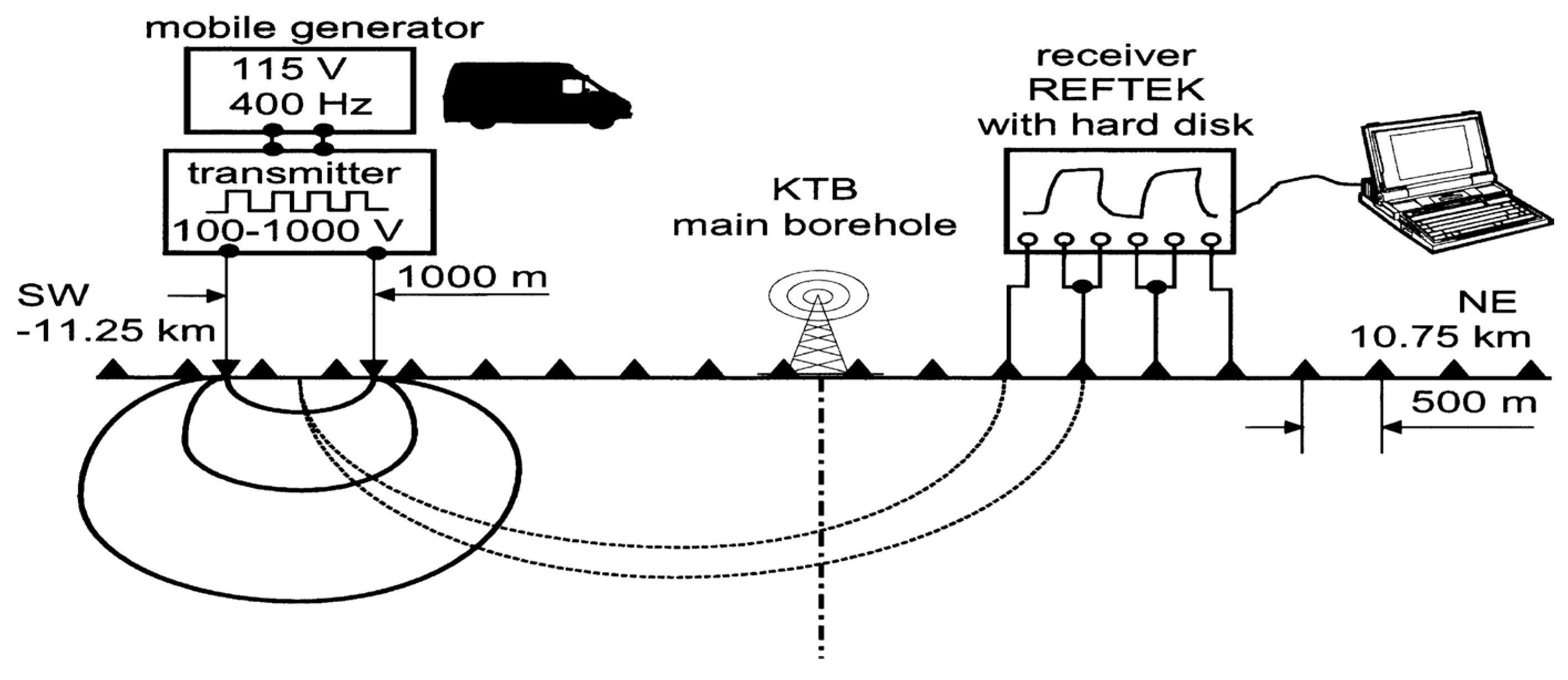
Figure 5.
Deep ERT image obtained close to KTB facility (Germany); the conductive anomaly in the central part of the profile is associated to the presence of a fault zone with fluids. (Reprinted with permission from [28], Copyright (2000), Wiley-Blackwell Publishing Ltd.).
Figure 5.
Deep ERT image obtained close to KTB facility (Germany); the conductive anomaly in the central part of the profile is associated to the presence of a fault zone with fluids. (Reprinted with permission from [28], Copyright (2000), Wiley-Blackwell Publishing Ltd.).

Figure 6.
ERTs carried out in the northernmost (ERT 1, 2 and 3) and southernmost (ERT 4, 5 and 6) part of the High Agri Valley basin. The relatively high resistivity contrast between the shallow alluvial deposits and the pre-Quaternary bedrock highlights the geometry of the fault-bonded basin. The resistivity zones on the shallow layers are associated with the presence of fans on the flanks of the basin. The shape of the basin floor is asymmetric and the maximum sediment thickness occurs along the northeastern margin (Reprinted with permission from [32], Copyright (2004), Elsevier).

Figure 7.
DERT image elaborated by the DCIP2D inversion code. Major features are labeled with letters. (A) represents alluvial deposits and the Messinian turbidite complex; (B) Unfractured calcareous block. The more resistive blocks are probably associated to Miocene units. Black dashed lines indicate presumed faults [36].

Figure 8.
(a) Model of the first ERT profile obtained using a Wenner-alpha array configuration; (b) ERT interpretation of the tomographic image with the bedrock/basin infill bodies and main faults highlighted (Reprinted with permission from [38], Copyright (2016) Oxford University Press).
Figure 8.
(a) Model of the first ERT profile obtained using a Wenner-alpha array configuration; (b) ERT interpretation of the tomographic image with the bedrock/basin infill bodies and main faults highlighted (Reprinted with permission from [38], Copyright (2016) Oxford University Press).

Figure 9.
(a): Results of the deep ERT tomographic inversion. (b) Coverage (log10) of the penetration depth (Reprinted with permission from [39], Copyright (2019) Oxford University Press).
Figure 9.
(a): Results of the deep ERT tomographic inversion. (b) Coverage (log10) of the penetration depth (Reprinted with permission from [39], Copyright (2019) Oxford University Press).
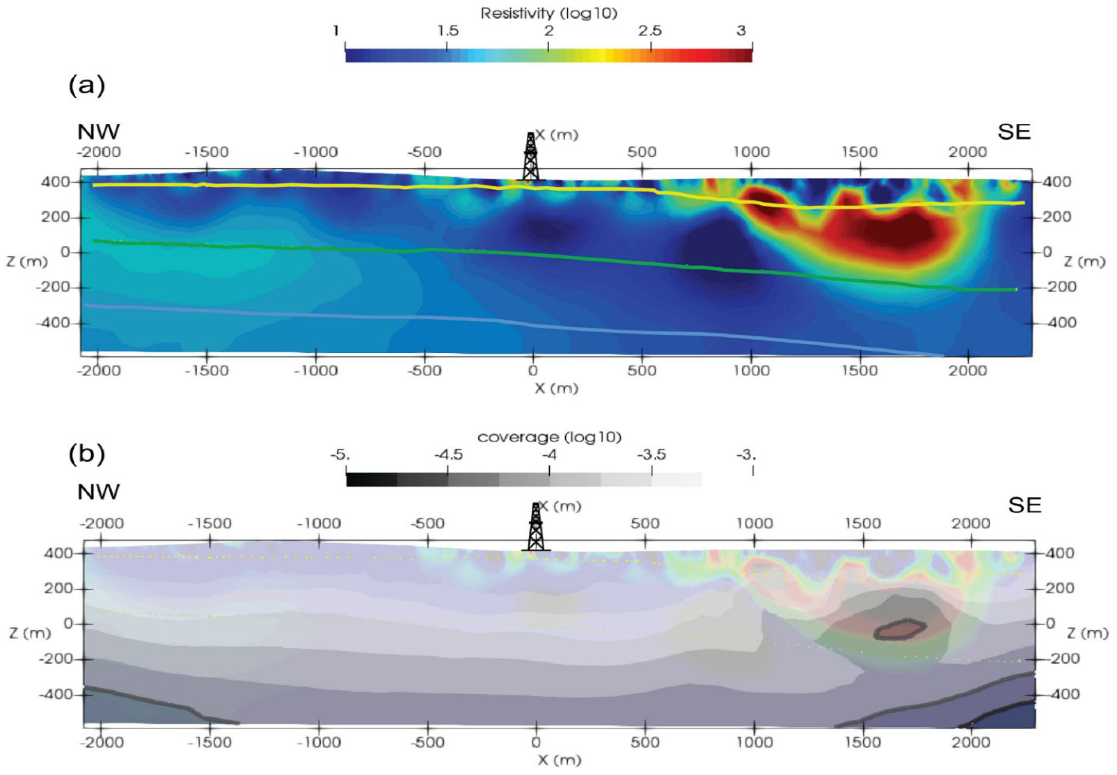
Figure 10.
3D representation of the interpreted model superimposed on the geological map of the slope. The squares represent the resistivity (log10) of the surface waters sampled in spring or at surface runoff locations. The black lines represent the major faults. (Reprinted with permission from [41], Copyright (2019) Oxford University Press).

Figure 11.
(a) Electrical resistivity 3D model obtained through the deep ERT imaging. (b) Electrical resistivity cross-sections along selected traces. (c) Map of the area resolved by the ER survey [42].
Figure 11.
(a) Electrical resistivity 3D model obtained through the deep ERT imaging. (b) Electrical resistivity cross-sections along selected traces. (c) Map of the area resolved by the ER survey [42].

Figure 12.
3D projection of the acquired deep electrical resistivity tomography data. Extracted cells with resistivities below 2.5 Ohm.m underneath the active vents highlight the area of collapse (dashed black arrows). The red-shaded area indicates the Watukosek fault system that intersects Lusi [43].

Figure 13.
(a) 3D SH-DERT; (b) Resistivity isosurfaces obtained using only surface electrodes; (c) 3D full-data DERT; (d) Resistivity isosurfaces obtained using both surface and borehole electrodes. (Reprinted with permission from [44], Copyright (2022, Elsevier).
Figure 13.
(a) 3D SH-DERT; (b) Resistivity isosurfaces obtained using only surface electrodes; (c) 3D full-data DERT; (d) Resistivity isosurfaces obtained using both surface and borehole electrodes. (Reprinted with permission from [44], Copyright (2022, Elsevier).


Table 1.
Simplified classification of the main characteristics (geological context, array configurations, algorithms for data processing and inversion, investigation depth) of the DERT applications presented and discussed in Section 3.
Table 1.
Simplified classification of the main characteristics (geological context, array configurations, algorithms for data processing and inversion, investigation depth) of the DERT applications presented and discussed in Section 3.
| Authors | Geological Context, Country | Array and Electrode Spacing | Processing; Inversion | Investigation Depth |
|---|---|---|---|---|
| Flores et al., 1997 | Geothermal, El Salvador | dipole–dipole, 500 m up to 1000 m | pseudosection | 2 km (pseudodepth) |
| Di Maio et al., 1998 | Volcanic, Italy | 500 m | stacking; pseudsection | 3 km (pseudodepth) |
| Storz et al., 2000 | Faults, Germany | dipole–dipole, 500 m | stacking; SIRT | 4 km |
| Colella et al., 2004 | Faults, Italy | dipole–dipole, 200 m | detrending, filtering and FFT; RES2DINV | 0.5 km |
| Balasco et al., 2011 | Geothermal, Italy | dipole–dipole, 400 m | stacking and FFT method; DCIP2D | 1.2 km |
| Pucci et al., 2016 | Faults, Italy | Wenner-alpha and pole–dipole, 40 m | X2IPI software for data filtering; RES2DINV | ~0.75 km |
| Carrier et al., 2019 | Geothermal, Switzerland | dipole–dipole, 50 m | Full-wave viewer software; BERT | ~1 km |
| Lajaunie et al., 2019 | Landslide, France | dipole–dipole, 50 m | Full-wave viewer software; BERT | 0.5 km |
| Troiano et al., 2019 | Volcanic, Italy | 100 m | Principal component decomposition, ERTlab3D | 0.4 km |
| Mazzini et al., 2021 | Volcanic, Indonesia | dipole–dipole, 50 m | Full-wave viewer software; BERT | 0.5 km |
| Rizzo et al., 2022 | Geothermal, Italy | dipole–dipole, 50 m | detrending, filtering and FFT; ERTlab | 1.6 km |
Publisher’s Note: MDPI stays neutral with regard to jurisdictional claims in published maps and institutional affiliations. |
© 2022 by the authors. Licensee MDPI, Basel, Switzerland. This article is an open access article distributed under the terms and conditions of the Creative Commons Attribution (CC BY) license (https://creativecommons.org/licenses/by/4.0/).
Share and Cite
MDPI and ACS Style
Balasco, M.; Lapenna, V.; Rizzo, E.; Telesca, L. Deep Electrical Resistivity Tomography for Geophysical Investigations: The State of the Art and Future Directions. Geosciences 2022, 12, 438. https://doi.org/10.3390/geosciences12120438
AMA Style
Balasco M, Lapenna V, Rizzo E, Telesca L. Deep Electrical Resistivity Tomography for Geophysical Investigations: The State of the Art and Future Directions. Geosciences. 2022; 12(12):438. https://doi.org/10.3390/geosciences12120438
Chicago/Turabian StyleBalasco, Marianna, Vincenzo Lapenna, Enzo Rizzo, and Luciano Telesca. 2022. "Deep Electrical Resistivity Tomography for Geophysical Investigations: The State of the Art and Future Directions" Geosciences 12, no. 12: 438. https://doi.org/10.3390/geosciences12120438
Note that from the first issue of 2016, this journal uses article numbers instead of page numbers. See further details here.