1. Introduction
A great number of Russian oil and gas fields are located in the Arctic region, where vast expanses, harsh climate, geotechnical, logistic, and infrastructure issues pose problems to the production and transportation of hydrocarbons. Particular risks are due to the presence of permafrost, as well as of sub- or intrapermafrost gas hydrates [
1,
2,
3]. Intrapermafrost gas hydrates at relatively shallow depths within 150 m can stay metastable for a long time due to self-preservation [
4,
5]. The dissociation of relict intrapermafrost gas hydrates deteriorates the bearing capacity and continuity of permafrost and causes excess pore pressure, leading to an explosive methane emission with the formation of crater landforms [
6,
7,
8,
9,
10,
11,
12].
The problem of thermal and mechanic interactions between production wells and permafrost was formulated in the 1970s, with the onset of development in the Russian Arctic petroleum provinces. The first models for estimating the size of thaw around wells appeared in the 1970–1980s [
13,
14,
15,
16,
17,
18,
19,
20,
21]. With various techniques available at present, the thermal field of permafrost around wells can be modeled as a function of user-specified temperatures inside wells [
17,
22,
23,
24,
25,
26,
27,
28,
29,
30,
31].
One of the key problems related to well completion in permafrost is the control of thaw subsidence and mechanic stability of wells. Correspondingly, the mechanic well–permafrost interaction has been modeled since the 1980s [
32,
33,
34,
35,
36]. Today, the mechanic and thermal issues associated with production from northern oil and gas fields are considered in publications and regulation documents of Gazprom [
19,
25,
26].
Several successes were achieved by foreign specialists in oil fields of the North Slope of Alaska, mainly, the Prudhoe Bay, where wellbore stability was principally ensured by solving the mechanical problem [
37,
38,
39]. This is caused by the specificity of the North American permafrost, which mostly consists of cemented sedimentary or coarse grain (boulders, cobbles, and gravels) rocks [
40]. This is fundamentally different from the approaches of Russian (or Soviet) specialists, who first always solved the thermal problem for the wellbore stability assurance because Russian permafrost (mainly north of Western Siberia) is represented by deep ice-rich dispersed sediments, which have high strength in the frozen state, but completely lose their bearing capacity after thawing.
According to the wealth of gained experience, the placement and operation of Arctic wells face serious engineering problems aggravated by weather conditions and related emergencies, which increase operational costs [
41,
42,
43,
44,
45,
46,
47,
48,
49,
50]. The existing models do not account for the interstitial free and clathrate gas components of permafrost and thermal impacts. Meanwhile, the emission of gas liberated by the dissociation of sub- or intrapermafrost gas hydrates in oil and gas fields is a frequent but poorly investigated event [
51,
52,
53]. Other problems include the formation of voids during drilling in permafrost, rapid thawing around wells that leads to soil subsidence, damage to casing and wellhead equipment upon freezing, hydrate or paraffin-hydrate clogging, etc.
Most of the previously conducted modeling was performed for ideal geological cases, without due attention to the real geocryological conditions of Arctic oil and gas fields. We formulate a problem for the forward modeling of the well–permafrost thermal interaction applied to the Bovanenkovo gas field in the Yamal Peninsula. The model accounts for the presence of relict gas hydrates in shallow permafrost as a key control factor of its thermal patterns [
54].
2. Thermal Interaction of a Well with Permafrost: Physical Problem Formulation
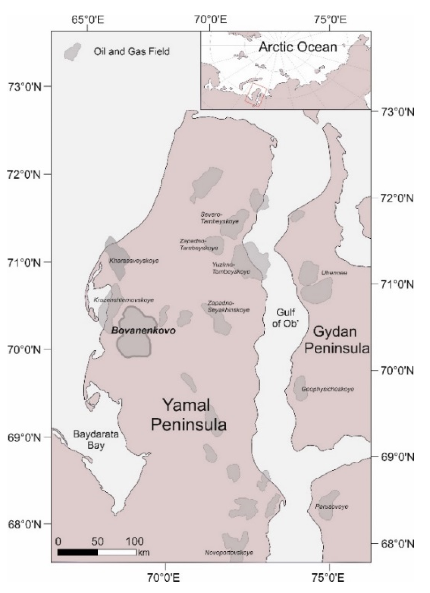
The Bovanenkovo gas field is located in the central part of the Yamal Peninsula (
Figure 1). Its geological and geocryological conditions have been well studied [
55,
56,
57].
This is an area of continuous ice-rich 140 to 230 m thick permafrost, with temperature ranging from −4 to −7 °C, composed of wet silt and clay silt. The contents of pore water and ice decrease depthward, with the total moisture varying from 40–45% in the upper part to 25–30% near the permafrost base. The soil is saline and freezes at ≤−2 °C. A The high gas saturation in the upper 130 m of permafrost is evident in spontaneous gas and shows during the drilling of geotechnical, test, and exploratory wells. The daily gas flow rates can reach hundreds or even thousands of cubic meters, possibly, due to the presence of metastable relict gas hydrates in shallow permafrost [
5,
10,
55,
58].
The well–permafrost interaction was simulated using data on the permafrost structure and physical properties from the Bovanenkovo gas-condensate field [
51]. The modeling domain extended to a depth of 550 m, while the permafrost thickness was assumed to be ~210 m. The model consisted of three layers (Layer 1, Layer 2, and Layer 3), with different user-specified thermal properties and an unfrozen water content at <0 °C (
Table 1;
Figure 2).
Layer 1, 0 to 150 m: Quaternary glacial-marine lean clay (mgII2–4), with relict methane hydrates possibly occurring in the 60–120 m interval; average moisture content 32%; freezing point is around −1 °C.
Layer 2, 150 to 250 m: Glacial-marine lean clay (mgI1); 22% moisture content; freezing point is −2 °C.
Layer 3, 250 to 550 m: Marine fat clay (P1-mK2); 23% average moisture content; freezing point is −2 °C.
The model parameters represented changes in the amount of unfrozen water in permafrost soils, as well as the enthalpy of phase transitions in pore gas hydrates (dissociation) and ice (melting). The modeling was run in Ansys Fluent in two steps.
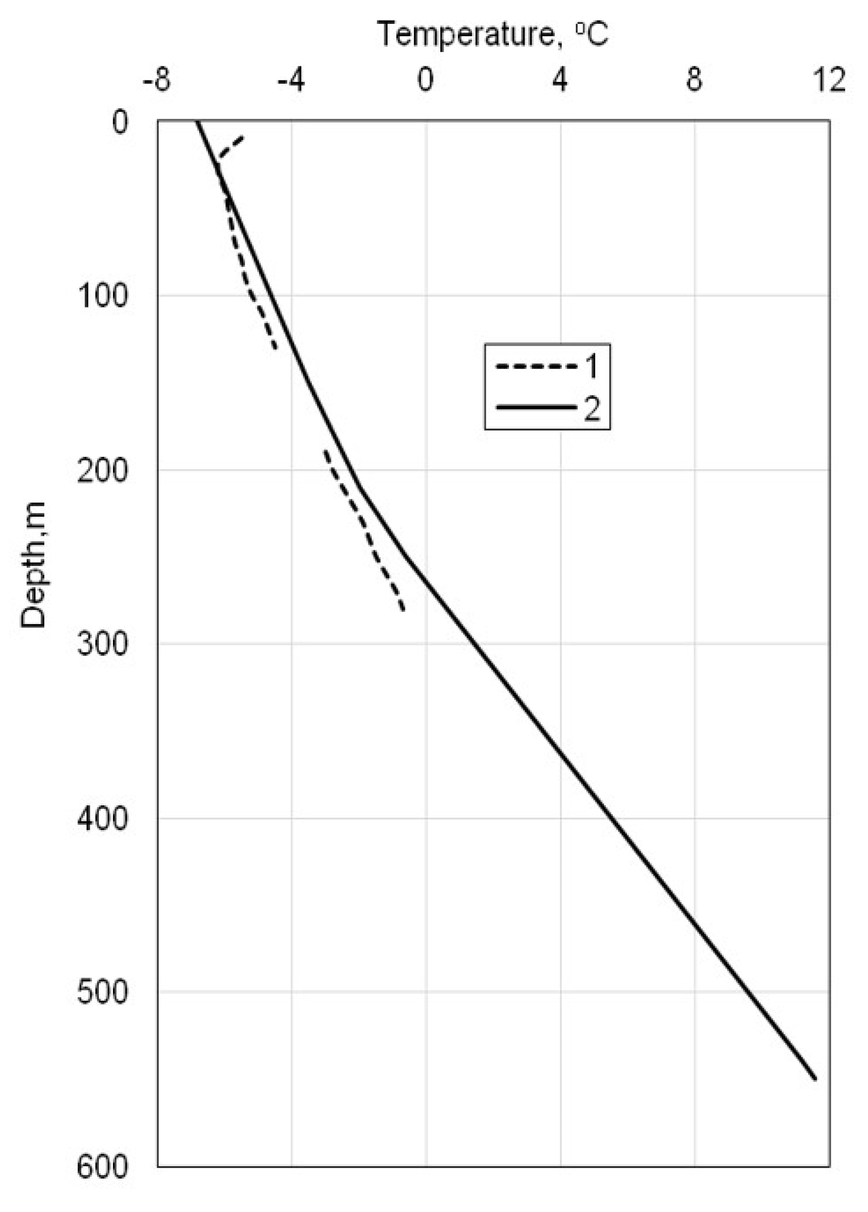
At the first step, the behavior of permafrost in the area of future drilling was predicted based on paleoclimatic scenarios [
59,
60], with reference to the modeled middle-late Pleistocene and Holocene permafrost evolution in the Yamal Peninsula. Then, present permafrost thickness and depthward temperature patterns were fitted to field data, while the lower boundary condition (deep heat flux) was allowed to vary. Thus, an estimated permafrost thickness, corresponding to the soil surface temperature −6.8 °C (upper boundary condition) and a heat flux of 49.17 mW/m
2 (lower boundary condition), was around 210 m, and the temperature-depth profile fitted the pattern of a well from the Bovanenkovo field (
Figure 3).
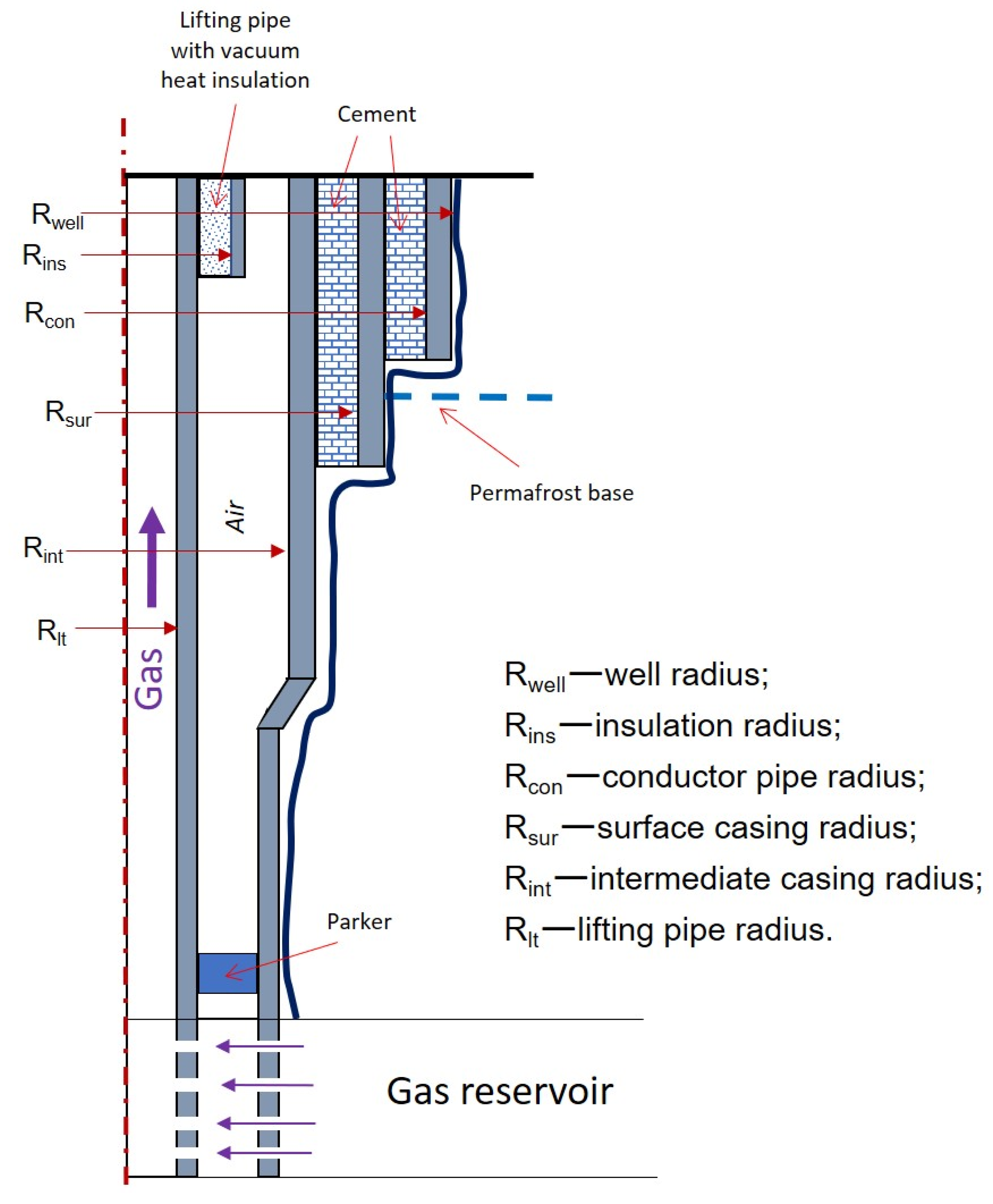
At the second step, modeling was performed for a well completion with three casing strings (
Figure 4;
Table 2): lifting pipe (model 168/114) with vacuum heat insulation to a depth of 55 m; conductor pipe to a depth of 120 m; surface casing to a depth of 450 m; intermediate casing reaching the reservoir; cement between the surface casing and conductor pipe and between the surface and intermediate casings. This design has been used in >50 m ice-rich permafrost of northern West Siberia [
25].
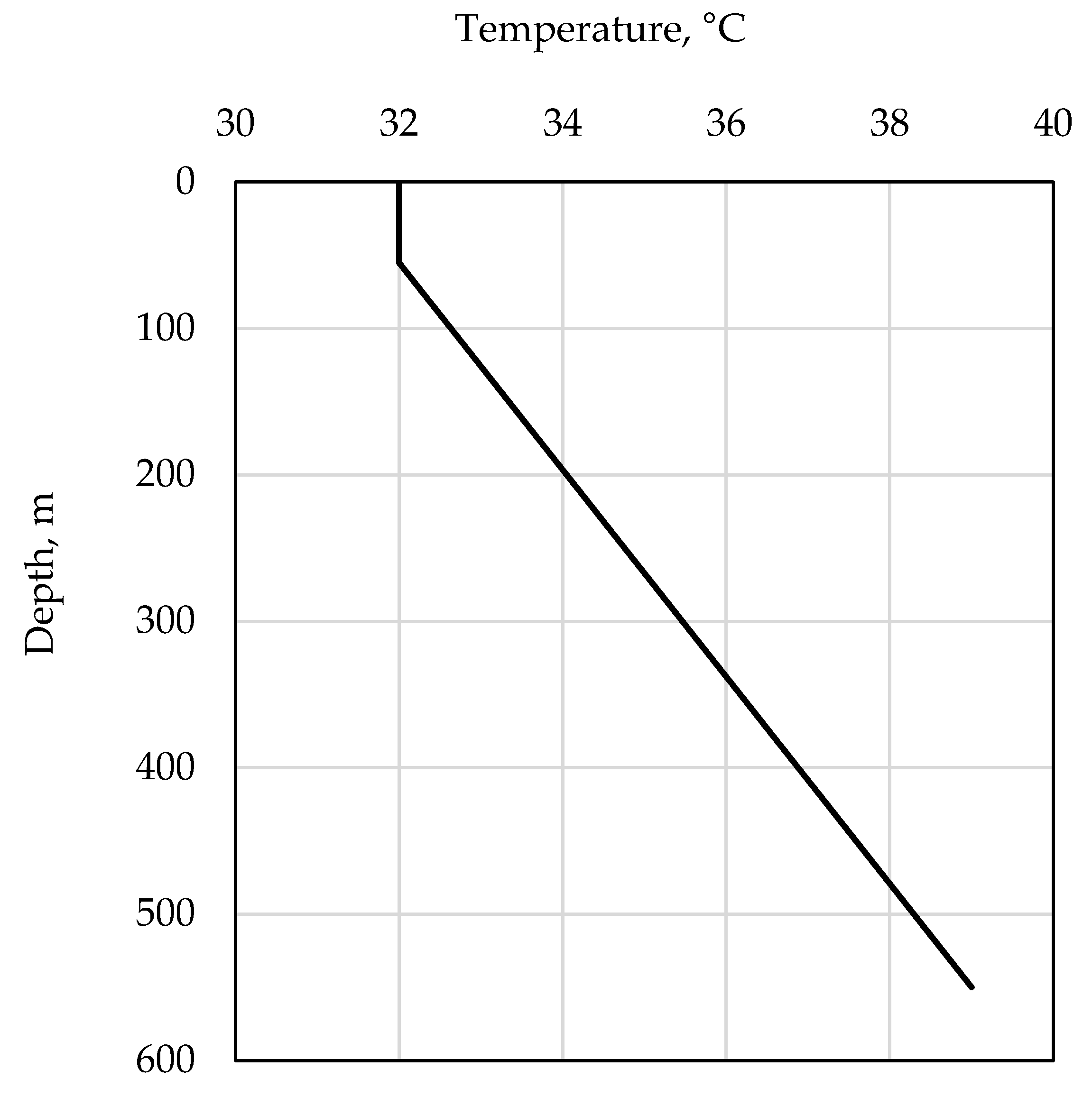
The 55 m heat insulation depth used in the model was common to some production wells at the Bovanenkovo gas field [
61]. The temperature on the lifting pipe/permafrost interface within the insulation interval was assumed to be constant at 32 °C. It was estimated to proceed from the reservoir temperature, local geothermal gradient, and gas flow rate. The gas temperature in the lifting pipe increased almost linearly with the depth to reach +39 °C at 550 m below the wellhead (
Figure 5). The gas reservoir is a Cenomanian sandstone at the depth interval of 1200–1400 m with a temperature of about +50 °C. The gas was recovered at a daily flow rate of ~400,000–500,000 m
3, and its pressure was ~10 MPa.
The steel casing was assumed to have a heat capacity of 600 J/(kg·K) and a thermal conductivity of 58 W/(m·K). The thermal conductivity of vacuum insulation was ~0.08 W/(m·K), and that of gas in the lifting pipe was 0.09 W/(m·K). The respective thermal properties of cement (2400 kg/cm3 density) were 840 J/(kg·K) and 1 W/(m·K).
The well–permafrost interaction was simulated using the enthalpy formulation for the Stefan problem [
62]. The Stefan solution, in this case, was a solution to a quasilinear thermal conductivity equation that expressed the conservation law within the modeling domain with regard to phase transitions (ice melting and gas hydrate dissociation). This approach was based on the previous models for estimating the thaw radius around producing petroleum wells [
60]. It accounts for variations in the content of unfrozen pore water in warming permafrost, as well as for the presence of intrapermafrost metastable gas hydrates.
The quasilinear thermal conductivity equation that expressed the conservation law within the modeling domain Ω
r with regard to phase changes, in the axisymmetric case, was
here
are, respectively, the spatial variables of the radius and depth;
is the time;
is the temperature;
is the thermal conductivity;
is the volumetric (effective) heat capacity. The effective heat capacity
in Equation (1) allowed for two types of phase changes: (i) the melting of pore ice and formation of free pore moisture (unfrozen water) at negative temperatures and (ii) the dissociation of metastable relict gas hydrates, which was likewise considered as a first-kind phase transition. The model represents a typical case of hydrate dissociation upon permafrost warming within −2.5 to −1.5 °C around a well, while the released water froze up immediately. The heat was consumed during dissociation but released during freezing, and the total heat budget was positive:
, where
are, respectively, the saturation (volume fraction), density, and specific latent heat of pore methane hydrate. As the temperature increased further, pore ice melted within the ranges −1.0 to −0.9 °C and −2.0 to −1.9 °C for Layer 1 and Layer 2, respectively.
The thermal properties of permafrost were specified using a model of a porous solid with interstitial space filled with a solid or liquid material with (or without) a free gas phase.
The input parameters for the problem, specified separately for each geological layer, were:
—density, specific heat, and thermal conductivity of solid particles, respectively. Thermal conductivity was calculated as a function of temperature, tabulated, or polynomial;
—density, specific heat, and thermal conductivity of fluid, respectively.
—porosity, phase composition (ice saturation, possibly depending on temperature according to the unfrozen water curve), specific heat of phase transitions, and the temperature at the beginning and end of phase transitions, respectively;
Properties of the fluid depending on its state (with possible regard for salinity), found via water and ice properties [
63,
64] as:
- density, effective heat capacity, and thermal conductivity of permafrost, respectively, found as:
Effective heat capacity associated with the freezing of unfrozen pore water was found as:
Equation (4) is applicable outside the range of pore moisture freezing and hydrate dissociation. The obtained effective heat capacity values (without free moisture) for Layers 1–3 are listed in
Table 2,
Table 3 and
Table 4. Blue and orange highlighted the temperature range with active phase transitions of pore ice–water and gas hydrate–ice, respectively.
In the presence of interstitial gas (either free or hydrate), Equation (3) included additional terms or factors:
where the volumetric fractions are related to as
, with temperature-dependent fractions of ice or gas hydrate
controlling the rate of the respective phase transitions [
65].
The dissociation of gas hydrates was given by:
Equation (6) is applicable outside the range of pore moisture freezing and unfrozen water.
Note, again, that the equation was valid only for negative temperatures, while the dissociation of gas hydrates at positive temperatures consumed latent heat , without the subtraction of latent ice formation heat.
The freezing of free moisture (Stefan problem) was expressed by Equation (4), with a stepwise ice content, but the iteration convergence requires smoothing of the step, for instance, by a linear function determined within a narrow (<0.1 °C) temperature range
, or in a more complicated way. Note that the phase change of free moisture was handled in a special
Fluent module inaccessible for programming, and, thus, missed from the effective heat capacity in (5) and (6) and respective
Table 3,
Table 4,
Table 5 and
Table 6.
The modeling domain Ωr is a rectangle (in cylindrical coordinates) bounded by the lifting pipe/air interface on the left and by the ground surface on the top, with its vertical and horizontal (radial) sizes of 550 m and 50 m, respectively.
Equation (1) was extended with a boundary and initial conditions of the first kind: the constant temperature of −6.8 °C on the ground surface and the temperature on the lifting pipe/air interface changing stepwise with depth (
Figure 4). Note that we used the first-kind boundary condition on the lifting pipe surface instead of the commonly applied third-kind one because the heat output in the problem was quite high.
The lower boundary conditions were fitted to the known permafrost thickness of 210 m by solving the steady-state problem for undrilled permafrost, and the solution (
Figure 2) was used as an initial condition. As a result, the heat flux was assumed to be constant, 49.17 mW/m
2, at the base of the modeling domain and zero along the side boundaries, provided that the thermal effect of the well remained within the <50 m radius for 30 years of operation.
The physical properties of the solid and fluid components of permafrost were modeled using the gravimetric water content
, as a weight ratio of all moisture types to dry soil, and the dry (soil skeleton) density
Thus, the porosity was found as
with
for soil porosity. Then, the unfrozen water saturation in the porous media (
) (
Figure 2) was calculated by the following formula:
, where
is a relative moisture content
.
The thermal parameters for modeling were chosen with regard to the presence of pore gas hydrates in permafrost, which increased its effective heat capacity and decreased thermal conductivity (
Table 4,
Table 5 and
Table 6). In the tables, the temperature intervals in which free moisture freezes
and hydrates dissociate are highlighted blue and orange, respectively.
Note that we used free moisture for all unfrozen water in the presence of gas hydrates at the respective depths, i.e., physically, it was the Stefan solution. Allowing for hydrate dissociation and ice melting according to the unfrozen water curve within the same temperature range would require other (e.g., kinetic) models of hydrate dissociation and would complicate the model for no reason.
The thermal properties missing from
Table 3,
Table 4,
Table 5 and
Table 6 were specified as standard values; the assumptions were:
= 333.4 kJ/kg for the latent heat of ice melting;
= 501 kJ/kg for the heat of hydrate dissociation. Hydrates dissociated between −2.5 and −1.5 °C (
Table 4), i.e., the phase transition of the metastable hydrate was assumed to be smoother than the ice melting, due to the algorithm features.
Note that the effective heat capacity of lean clay was higher in the presence of pore hydrates (orange in
Table 4,
Table 5 and
Table 6).
The calculations were run on a non-uniform rectangular grid of more than 1000,000 nodes in total, with the minimum radial spacing (0.4 mm) near the lifting pipe/air interface. The depth grid spacing varied from 0.1 m near the ground surface to 10 m near the model base.
3. Results and Discussion
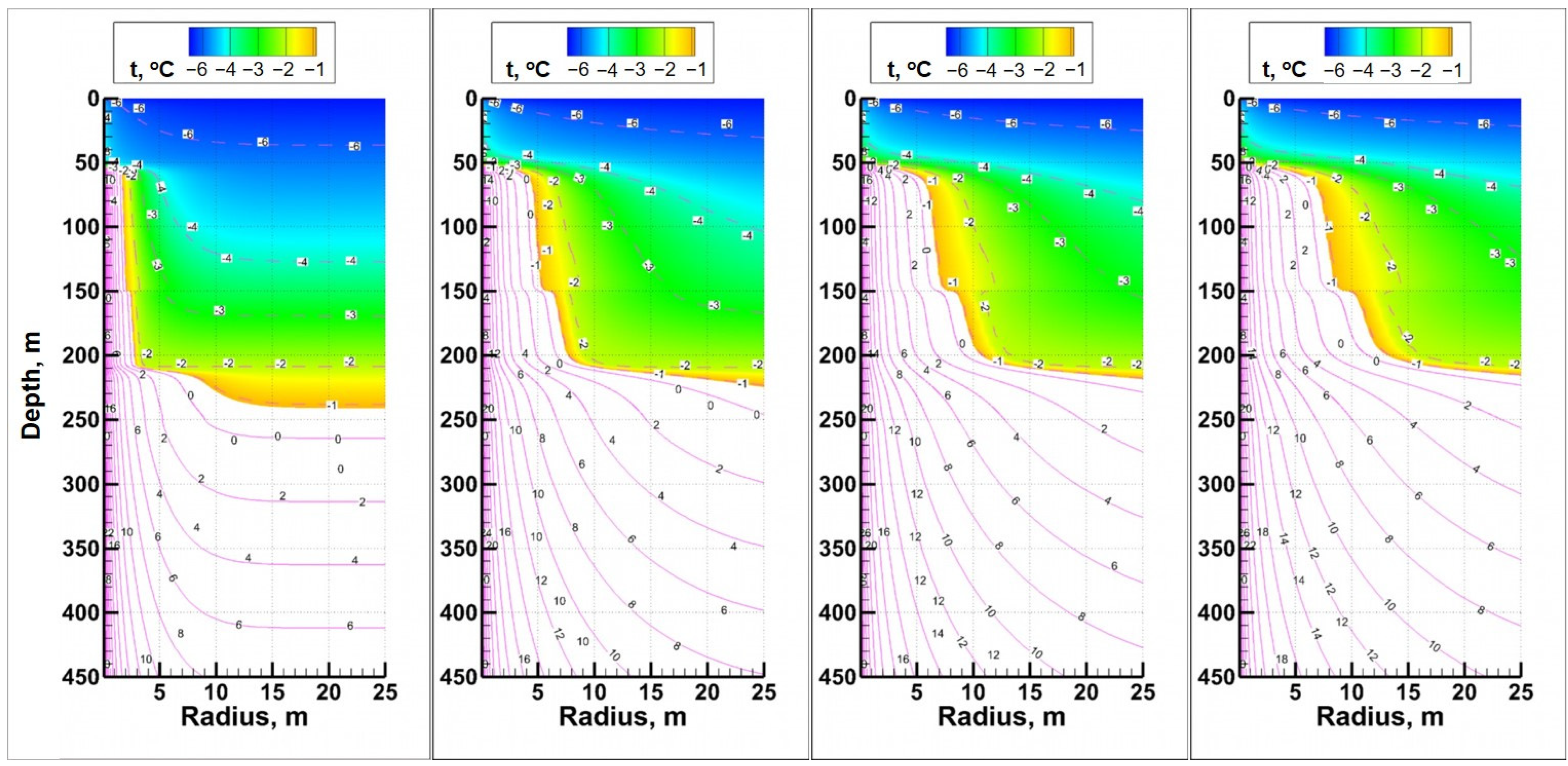
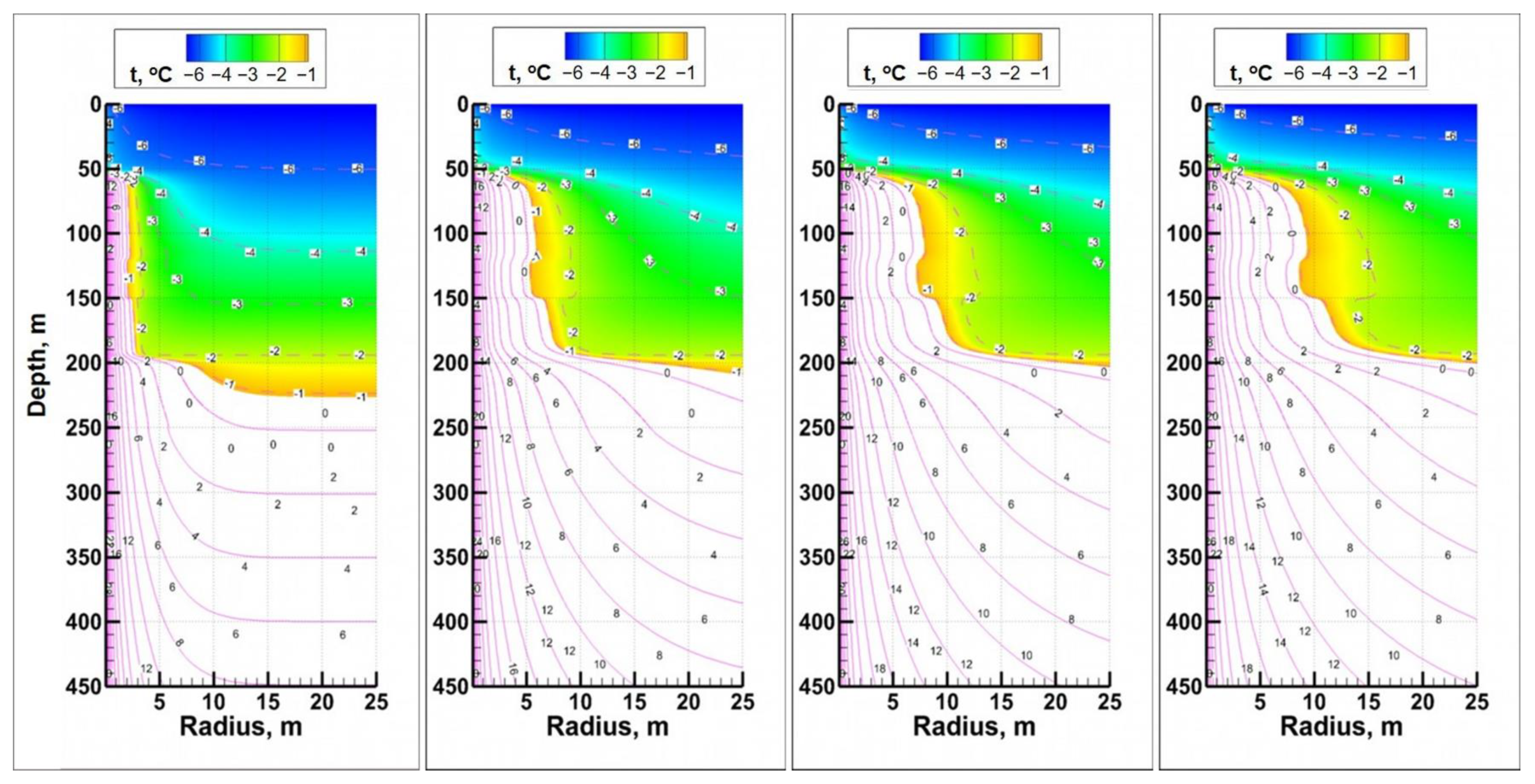
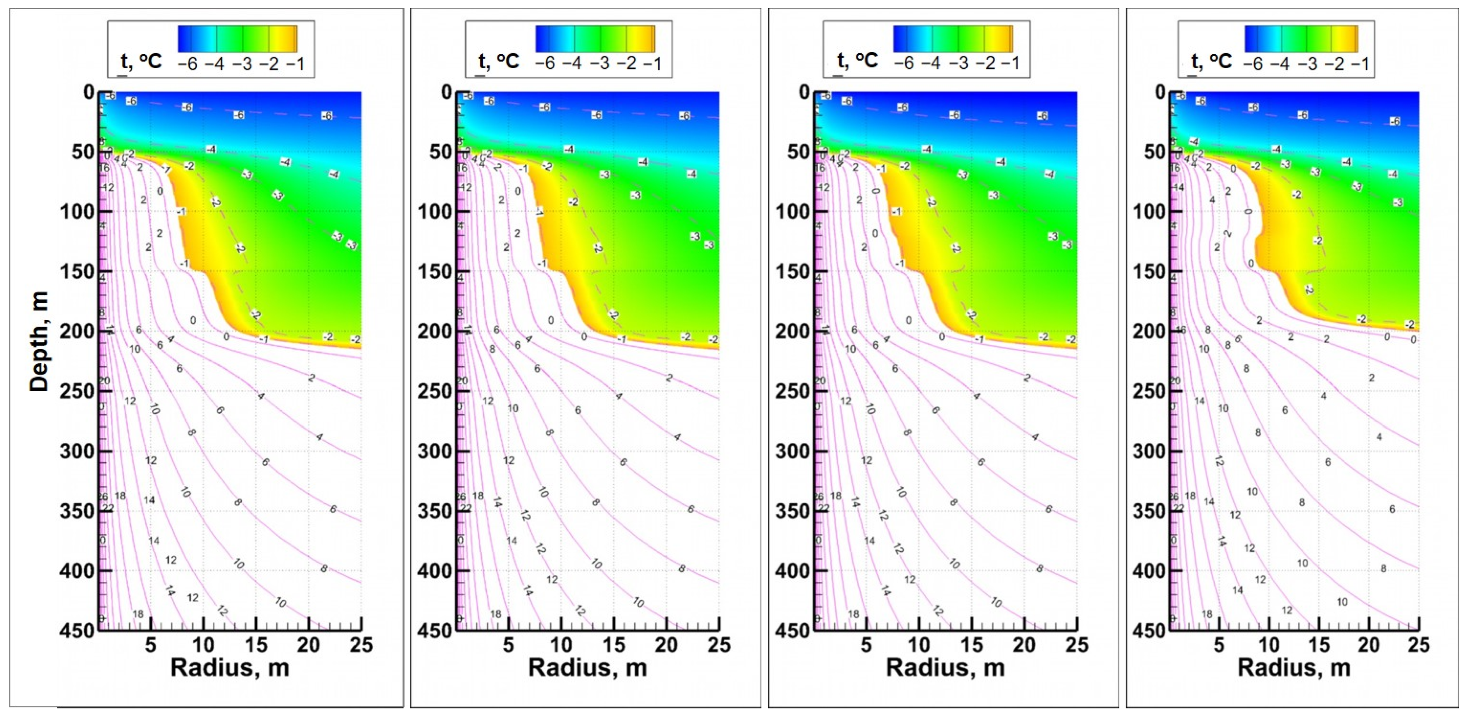
The thermal interaction of a producing gas well with permafrost was modeled for different pore fluid compositions and saturation values, within the 60 to 120 m depth interval (
Figure 6,
Figure 7 and
Figure 8).
Case 1: Relict gas hydrates, with 20% hydrate saturation (
) and 80% ice saturation (
), i.e., 100% of the pore space was filled with gas hydrate and ice. This saturation value was chosen proceeding from experiments on methane hydrates prone to self-preservation [
5].
Case 2: Relict gas hydrates, with 20% hydrate saturation (
) and 50% ice saturation (Si), i.e., 70% of the pore space was filled with gas hydrate and ice; plus, a 30% gas saturation (
). The presence of 20 to 30% of free pore space in permafrost that contains metastable gas hydrates was observed earlier in experiments on hydrate self-preservation [
3,
5].
In other cases, hydrate saturation was = 40% or zero at = 100%.
In all cases, the thermal conductivity of permafrost depending on hydrate saturation was specified proceeding from earlier experimental results [
54,
66].
The predicted thaw radius in hydrate-bearing permafrost around petroleum wells operating for 30 years may reach 7–10 m at 32 °C on the inner surface of a noninsulated lifting pipe till a depth of 55 m, and 12–15 m below this depth within the modeling domain. The heat insulation demonstrated its high efficiency; the permafrost around the well with the insulated lifting pipe (down to 55 m) could hold frozen for the whole lifespan of 30 years (
Figure 9).
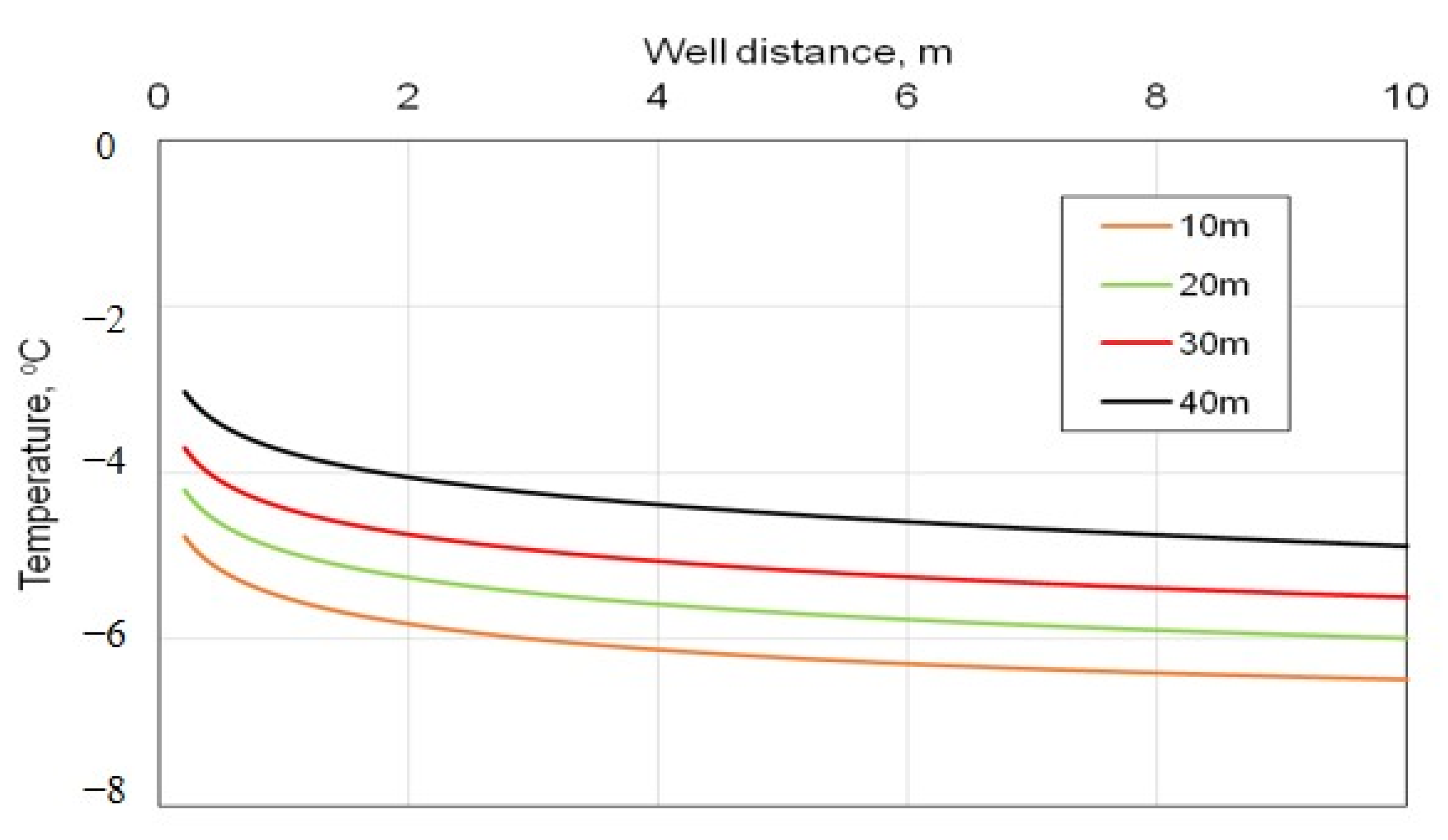
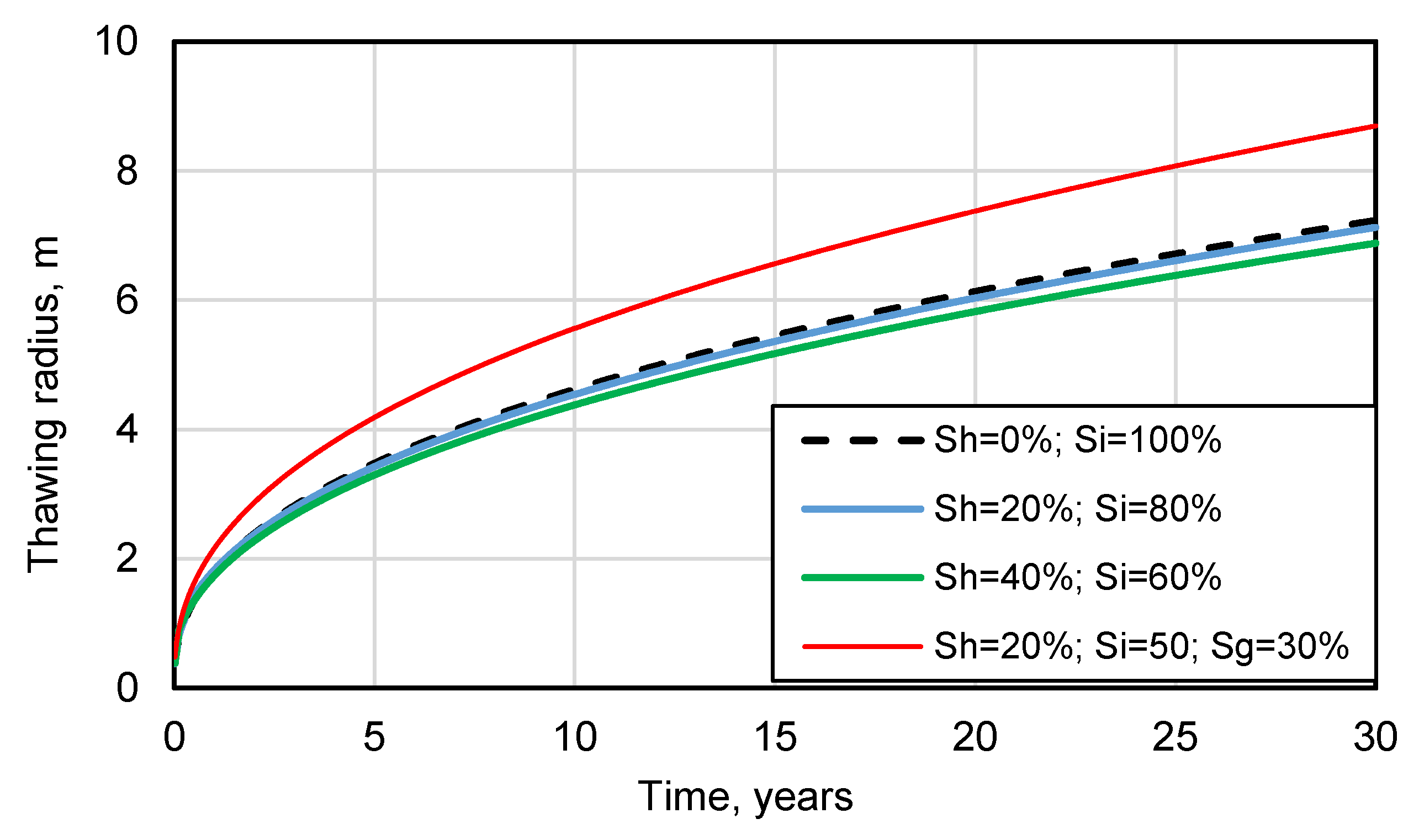
The thaw radius in permafrost-bearing gas hydrates depends on the total
Sh +
Si saturation (
Figure 10), that is, about 25% larger in the case of
= 70% than at
= 100%. The reason is that the presence of free pore space filled with methane (30% in our case) decreased the phase transition enthalpy for both ice and gas hydrate and, thus, accelerated the thawing.
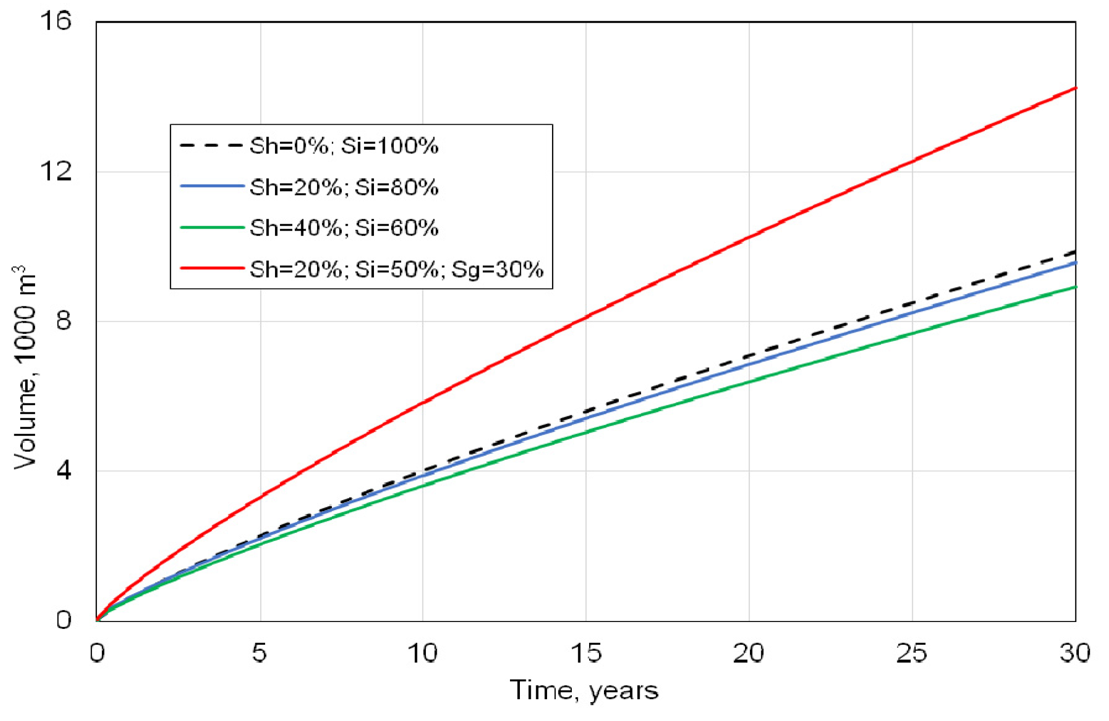
The thaw size in permafrost within the 60–120 m (
Figure 11) increased almost linearly with time (R
2 ≥ 0.99 for all fluid types). This is an illustration of quasiparabolic self-similar asymptotic thaw behavior after short initial heating till the end of the 30 yr well lifespan.
Pore gas hydrates turned out to only slightly affect the thawing rate; the thawing of permafrost with = 20% was <5% slower than in the absence of hydrates. This, apparently, unexpected result may be due to the starting conditions of about −5 °C permafrost temperature and 20% chosen according to field and laboratory experimental evidence from the Bovanenkovo field. The thawing was only slightly slower also at = 40% and + = 100%. As shown by more detailed studies, the effect of the hydrate component on the thawing rate is additionally controlled by thermal conductivity, which is inversely proportional to the hydrate saturation and initial permafrost temperature. On the other hand, thawing decelerated due to heat flux toward colder rocks. However, these issues require special consideration and are planned to be the subject of a separate study.
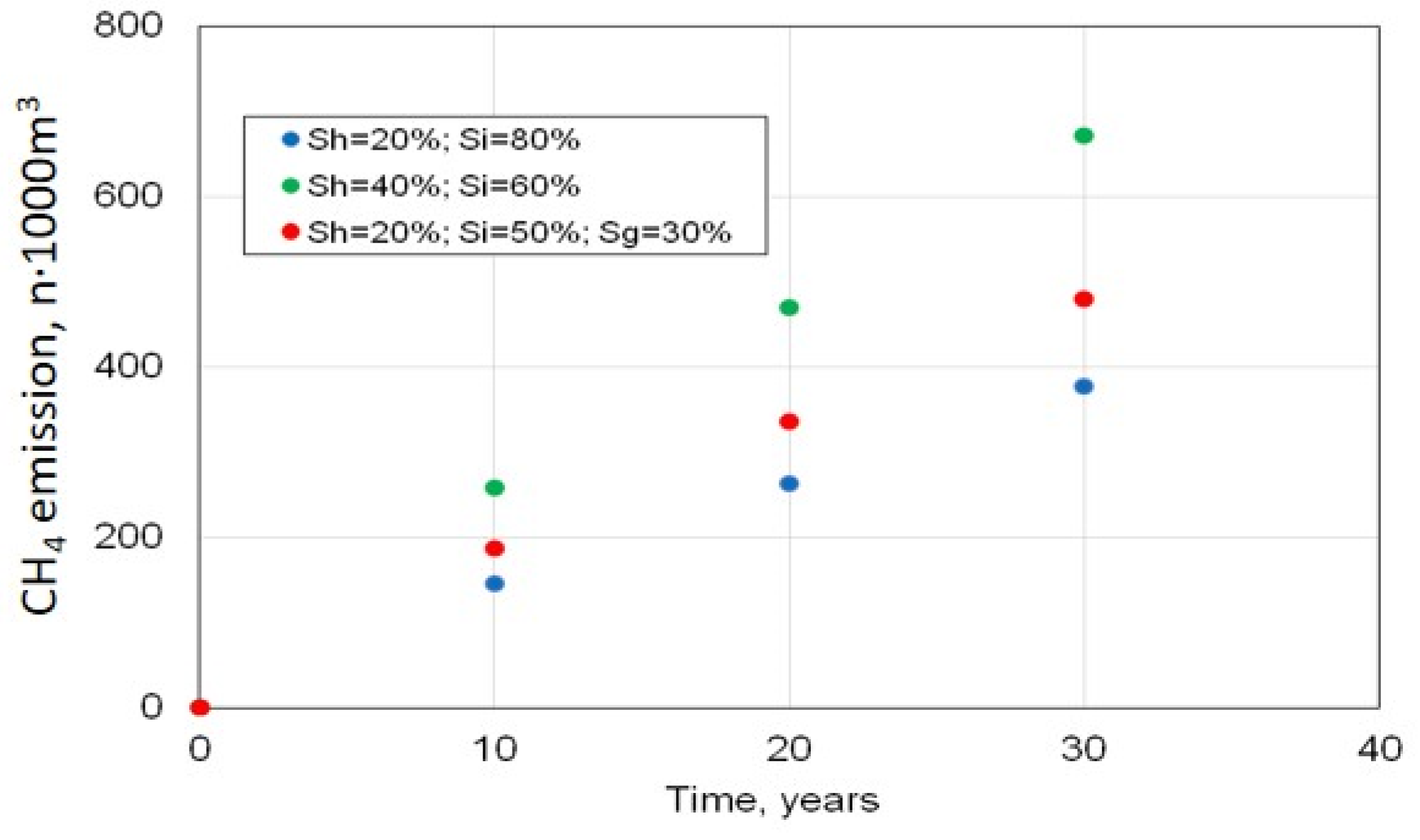
As predicted by the model, methane emission from permafrost that contained 20% of metastable pore gas hydrates could reach 400,000 to 500,000 m
3 after 30 years of gas production, corresponding to a daily emission of 50 m
3 (
Figure 12).
The amount of methane emission from hydrate-bearing permafrost exposed to warming upon the interaction with petroleum wells depends on the thaw size, as well as on the temperature and saturation (with hydrate and ice) of permafrost around the casing. The saturation, in turn, affects the thawing rate of permafrost via its thermal properties. For the considered cases, the potential emission became 80% greater as the hydrate saturation increased from 20 to 40%, but the increment was only 30% in the case of 20% hydrate saturation.
4. Conclusions
Active gas emission from permafrost associated with drilling and petroleum production in northern West Siberia, including the Yamal Peninsula, is due to the presence of intrapermafrost metastable (relict) gas hydrates. The thermal interaction of petroleum wells with hydrate-bearing permafrost was simulated in terms of the enthalpy formulation of the Stefan problem, with regards to variations in the amount of unfrozen pore water at negative temperatures, the dissociation of gas hydrates, and the heat of ice and hydrate phase transitions. The solution was reduced to a quasilinear thermal conductivity equation with a temperature-dependent heat capacity and thermal conductivity of permafrost.
The modeling was performed for a three-string well, with a vacuum heat-insulated a gas lifting pipe to a depth of 55 m, which was embedded in permafrost containing gas hydrates in the 60–120 m depth interval. The model parameters and boundary conditions were chosen with reference to evidence from the Bovanenkovo gas-condensate field.
The modeling predicted the thaw radius around a production well in hydrate-bearing permafrost to reach 7–10 m to 10–12 m in the upper and lower parts of the modeling domain, respectively, for a well lifespan of 30 years. However, almost no thawing would occur over 30 years of production if an insulated lifting pipe was used (down to 55 m).
The thaw radius mainly depended on the total hydrate and ice saturation, being greater in hydrate-bearing permafrost with incomplete saturation than in the case of a pore volume 100% filled with ice and gas hydrates.
Methane emission from degrading hydrate-bearing permafrost for 30 years of gas production in the Bovanenkovo gas-condensate field may reach 400,000 to 500,000 m3 in the absence of heat insulation. Meanwhile, the well design with insulated tubing can prevent thawing and the emission of methane, which can cause a twenty-five times greater greenhouse effect than CO2.


 ,
, 


