Mapping Gully Erosion Variability and Susceptibility Using Remote Sensing, Multivariate Statistical Analysis, and Machine Learning in South Mato Grosso, Brazil

Abstract

In Brazil, the development of gullies constitutes widespread land degradation, especially in the state of South Mato Grosso, where fighting against this degradation has become a priority for policy makers. However, the environmental and anthropogenic factors that promote gully development are multiple, interact, and present a complexity that can vary by locality, making their prediction difficult. In this framework, a database was constructed for the Rio Ivinhema basin in the southern part of the state, including 400 georeferenced gullies and 13 geo-environmental descriptors. Multivariate statistical analysis was performed using principal component analysis (PCA) to identify the processes controlling the variability in gully development. Susceptibility maps were created through four machine learning models: multivariate discriminant analysis (MDA), logistic regression (LR), classification and regression tree (CART), and random forest (RF). The predictive performance of the models was analyzed by five evaluation indices: accuracy (ACC), sensitivity (SST), specificity (SPF), precision (PRC), and Receiver Operating Characteristic curve (ROC curve). The results show the existence of two major processes controlling gully erosion. The first is the surface runoff process, which is related to conditions of slightly higher relief and higher rainfall. The second also reflects high surface runoff conditions, but rather related to high drainage density and downslope, close to the river network. Human activity represented by peri-urban areas, construction of small earthen dams, and extensive rotational farming contribute significantly to gully formation. The four machine learning models yielded fairly similar results and validated susceptibility maps (ROC curve > 0.8). However, we noted a better performance of the random forest (RF) model (86% and 89.8% for training and test, respectively, with an ROC curve value of 0.931). The evaluation of the contribution of the parameters shows that susceptibility to gully erosion is not governed primarily by a single factor, but rather by the interconnection between different factors, mainly elevation, geology, precipitation, and land use.

1. Introduction

The development of gullies is a major problem in Brazil, both in rural areas, where it can result in considerable net soil loss and change river baseflow, and in urban areas, where it threatens infrastructure and populations [1]. These are often impressive phenomena in terms of volumes of displaced soil cover [2]. While it is recurrent to see the formation of gullies associated with anthropic activities, some theories mention an ancient process that had its share of contribution in the morphology of Brazilian landscapes [3,4]. Today, both anthropic pressure and the modification of environmental conditions due to global climate change (especially the increase in extreme events) are likely to accelerate erosive processes. A better understanding of the role of the parameters that influence gully development is an important challenge that should lead to the elaboration of relevant vulnerability maps of land covers.

As this is a problem with a strong environmental and social impact, this concern in the Brazilian earth sciences community is not new, since reference works on this topic date back to the 1960s and 1970s with the works of Tricart [5] and Christofoletti [6], later taken up by Ross [7]. The soil cover fragility maps developed are based on various intrinsic criteria such as bedrock, relief, soil type, vegetation cover, land cover, and extrinsic criteria such as precipitation (average, cumulative, and intensity of events) or anthropogenic factors (urbanization, modification of drainage networks, road construction, etc.). Although several authors mention a case-specific adjustment of the models [8], in the vast majority of works, the study of gully formation and evolution is based on a uni-factorial approach, taking into consideration the major factors of water erosion mentioned above. Thus, the development of gullies is generally approached locally and case by case, often being limited to a descriptive aspect of the possible causes of erosion. The major factors favoring gully appearance or development are identified, but in the natural and anthropized environment, these different factors are often correlated to varying degrees, correlation that is variable in space. As a result, a complex determinism may be hidden behind a partial correlation between the occurrence of this type of erosion and a factor or criterion studied separately from other descriptive parameters of the environment. In this context, few works have attempted to measure the multifactorial determinism of gully occurrence, i.e., the different factors including the possible links between these different factors.

New environmental analysis tools such as remote sensing can provide substantial databases that can be processed by multivariate statistical procedures [9]. In the past decade, studies aiming at creating erosion susceptibility maps through statistical, machine learning, data mining, or multi-criteria decision analysis methods have multiplied. Machine learning methods such as multivariate discriminant analysis (MDA), random forest (RF), logistic regression (LR), support vector machine (SVM), and others have recently been implemented, for example, to understand the parameters controlling the development of drainage network types, urban flooding, landslides, soil subsidence, snow avalanches, and gully erosion [10,11,12,13,14,15,16,17,18,19,20]. These methods have demonstrated their superiority over traditional statistical-based techniques by having the ability to model highly dimensional and non-linear data sets, allowing complex environmental interactions to be evaluated [9,21,22]. Taking advantage of these recent tools, there are studies analyzing gully morphometry based on their fractal dimension [23,24], but to our knowledge, such databases have only been slightly developed to better understand erosive systems, specifically in the case of gullying in Brazil [25].

The aim of this work was precisely to investigate the determinism of gully development by a multifactorial approach that could in turn be used to estimate the risk of occurrence of this erosive phenomenon. Two approaches are combined here, including a multivariate statistical analysis (principal component analysis (PCA)), whose objective is to reduce the dimension of the data space, and to reveal independent macro-parameters responsible for gully development. Susceptibility maps were drawn using various machine learning algorithms: multivariate discriminant analysis (MDA), classification and regression tree (CART), logistic regression (LR), and random forest (RF). The selected site for this study was the Rio Ivinhema basin in the South Mato Grosso State, an area where the development of gullies is pronounced and displayed as a priority by decision makers.

2. Materials and Methods

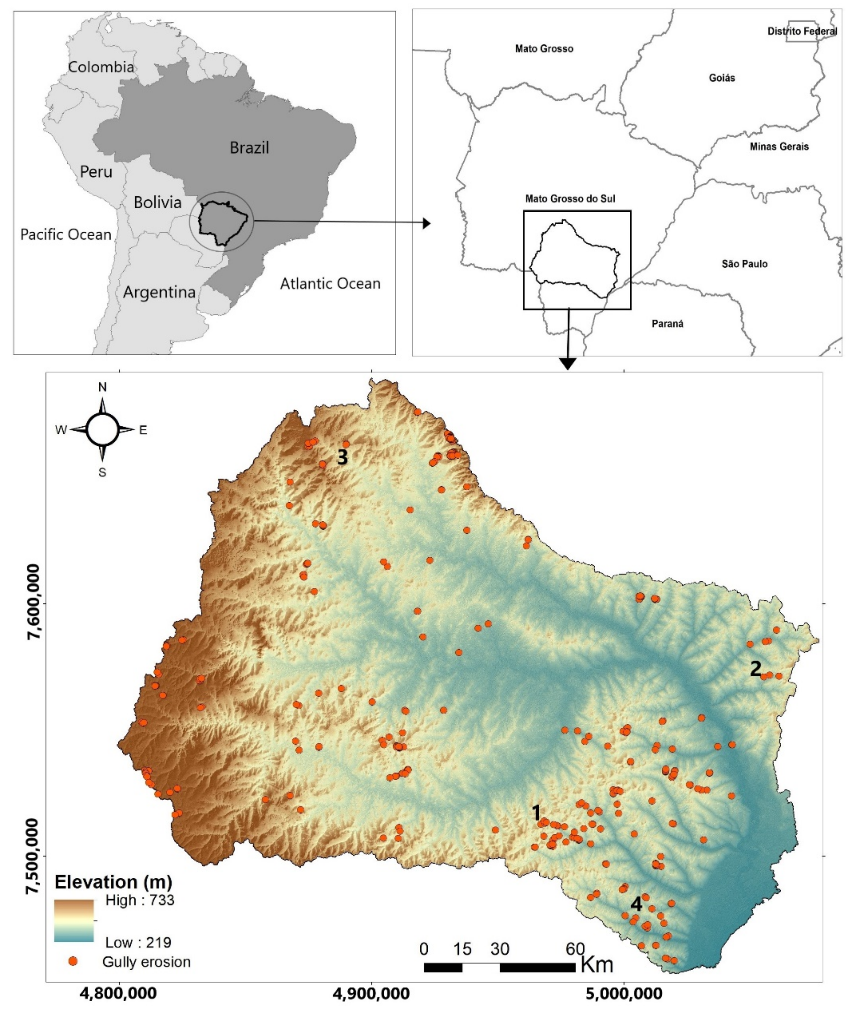
2.1. Study Area

The Ivinhema River (46,689 km²), a sub-basin of the Paraná River basin, is located in the southern part of the South Mato Grosso state in Brazil (Figure 1). It is limited to the west by the Serras das Araras, de Camapuã, and part of the Serra de Maracajú. The Ivinhema River (491.65 km long) springs in the municipalities of Rio Brilhante, Angélica, and Nova Alvorada do Sul, and flows 490 km to its confluence with the Paraná River near the city of Naviraí. The altitude of the basin varies from 800 m to 300 m a.s.l., and three classes of relief can be distinguished, namely, alluvial plains, gentle hills, and broad hills. The Ivinhema River is responsible for a significant part of the Quaternary alluvium sediment load deposited in the Paraná Valley. The Ivinhema basin is fully integrated into the geological context of the intra-cratonic sedimentary Paraná basin (1,500,000 km²), covering part of the territories of Brazil, Argentina, Uruguay, and Paraguay [26]. Three geological formations are found in the basin, namely, the Mesozoic formation of the Caiuá Group, the Serra Geral formation, and Quaternary alluvial deposits. The Caiuá Group consists of reddish quartz sandstone with a bimodal texture (very fine and coarse grains). The thickness of this formation does not exceed 150 m and the lithology is uniform in the whole basin. The formation is interpreted as having been deposited in a fluvial environment at the base, and eolian at the top [27]. The Serra Geral Formation consists of magmatic rocks related to fissural volcanism events and intrusion, whose maximum intensity occurred at the beginning of the Cretaceous period and extended to the Tertiary. In the study area, two main soil formations can be found: a purple latosol with clay to heavy clay texture, developed from the basalt of the Serra Geral geological formation in the upper basin, and a dark red latosol with clay texture, developed from the sandstone of the Caiuá formation in the lower part of the basin. The climate is tropical (Aw in the Köppen-Geiger classification), with an average annual temperature of 23 °C. The average annual rainfall ranges from 1400 mm in the northeast of the basin to 1600 mm in the southern part.

2.2. Input Variables Map

2.2.1. Gully Erosion Inventory

In Brazil, a distinction is made between ravina-type and voçoroca-type gullies. The former present a V-shaped profile, an elongated form, and are generally not very deep (0.5 m to a few meters). When erosion reaches the water table, the profile evolves into a U-shape due to surface erosion combined with deep erosion, and the gully takes the name of voçoroca. The erosion widens and may then continue in various directions and lose its elongated shape. The ravinas often turn into voçorocas from the bottom of the slopes, that is to say, closer to the hydrographic network where the water table is reached at lower depth. In this study, the term “gully” includes both ravinas and voçorocas. Ravina-type and voçoroca-type gully will be specified for their distinction when necessary. For the compilation of the database, two location classes were considered based on the presence (G points) or absence (non-G points) of gullies. These locations were identified based on the history of gully erosion incidence and the interpretation of satellite images on Google Earth (Figure 2). Although random sampling of non-G points leads to some artefacts in the use of machine learning modeling, it is a drawback that is almost impossible to eliminate [13]. In total, the database includes 800 georeferenced observations (400 G points and 400 non-G points). Figure 1 shows the location of the G points.

2.2.2. Selection of Environmental Parameters

In order to take into account a wide spectrum of geo-environmental factors that may influence the development of gullies [4,24,28,29], and more specifically under humid tropical climate, thirteen parameters were selected. These are elevation, slope, exposure, landform curvature, topographic wetness index (TWI), topographic position index (TPI), land cover, geology, drainage density, distance to rivers, distance to roads, soil type, and rainfall.

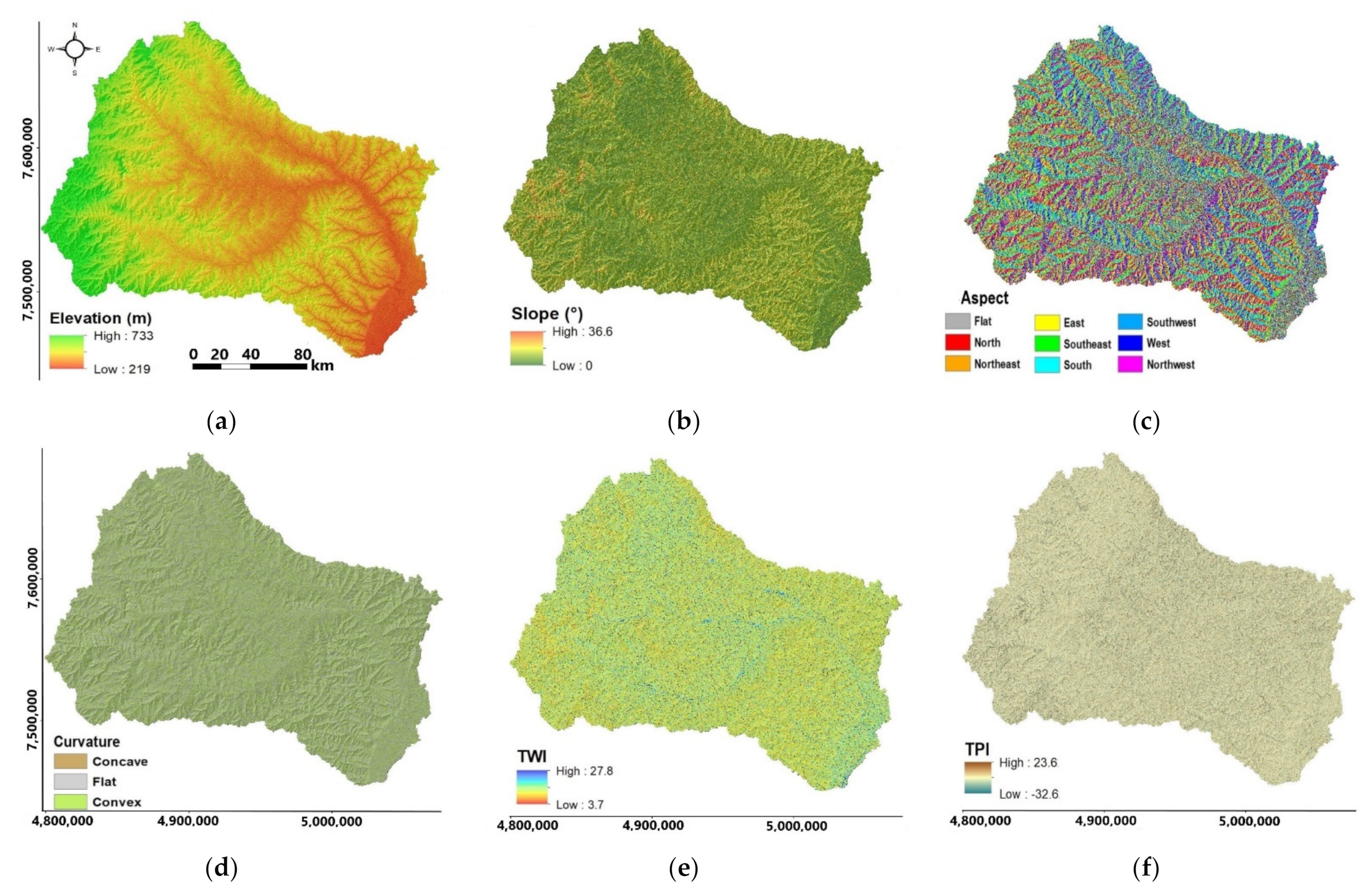
• Elevation is one of the most important factors affecting erosive phenomena with, in general, a positive relationship between elevation and the formation of gully and rill erosion [30]. The elevation map (Figure 3a) is derived from a 30 m resolution SRTM digital elevation model (DEM) obtained from the USGC Earth explorer website.
• Erosion is influenced by the slope gradient, a major physiographic feature [28,31]. Slope influences flow velocity and thus vulnerability to surface erosion. The slope map (Figure 3b) was determined using GIS from the 30 m resolution DEM.
• Exposure (frequently referred to as Aspect, Figure 3c) is defined as the direction of maximum slope. This parameter indirectly affects gully erosion as it controls microclimate, sun exposure time, moisture retention, evapotranspiration, weathering rates, vegetation cover, and denudation processes [15,32,33]. This parameter has also been calculated from the 30 m resolution SRTM DEM.
• Landform curvature is a factor in stormwater runoff [15,19,24]. Three categories were distinguished from the 30 m resolution DEM: concave, convex, or flat surfaces (Figure 3d).
• The topographic wetness index (TWI) represents the water accumulated in each pixel of the study surface [15]. It reflects the effect of topography on the distribution and zonation of saturation sources that may generate runoff (Figure 3e) [32,34,35]. TWI is calculated using a DEM (cell size = 30 m) and several GIS software tools to calculate slope, flow direction, flow accumulation, and slope angle [36].
• The topographic position index (TPI) indicates the upper and lower parts of the landscape, represented by the difference in elevation in each DEM cell (30 m) relative to the average elevation of surrounding cells [32]. Ridges and depressions are characterized by positive and negative values, respectively (Figure 3f). The TPI index results from comparing the elevation of each cell in a DEM with the average elevation of a specified neighborhood around that cell. The TPI is positive when the cell is higher than its surroundings (ridges and hilltops), and negative for depressed features such as valleys.
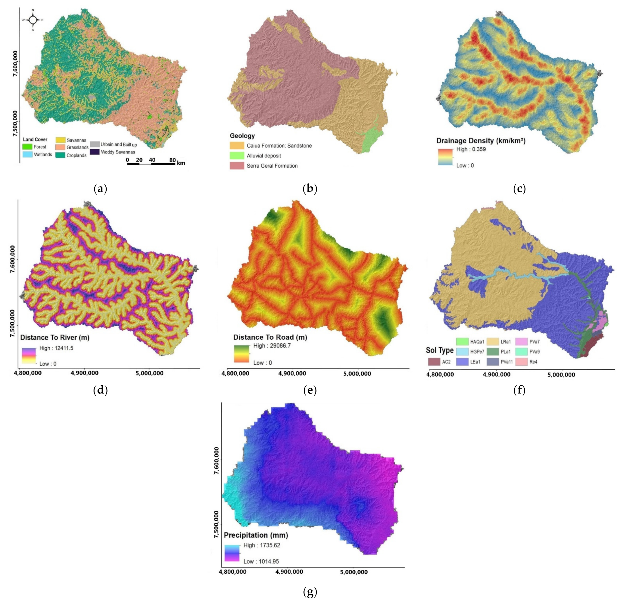
• Land cover and use can directly affect erosion [24]. The development of gullies is sometimes analyzed as an ancient phenomenon that has had its share of contribution to the morphology of Brazilian landscapes [3], but there are many studies that attest to the role of anthropogenic activities in contributing to and accelerating erosive processes [37]. Previous analysis, however, recognized that the effects are not always significant [25]. Therefore, a land cover map was made (Figure 4a) from the Moderate-Resolution Imaging Spectro-radiometer (MODIS) Land Cover Type 1 with a resolution of 500 m that has been resampled to a resolution of 30 m. The coding used for the land cover parameter is as follows: 1 = urban and built up, 2 = croplands, 3 = wetlands, 4 = grasslands, 5 = woody savannah, 6 = savannah, and 7 = forest.
• Geology is a critical parameter influencing erosive processes due to the strength of the rocks and soil formations that develop there, and the presence of lithological discontinuities [19,24]. Geological data of the study area were obtained from CRPM [38]. The three dominant geologic units are Quaternary alluvial deposits, basalts of the Serra Geral formation, and sandstones of the Caiuá formation (Figure 4b). The following code was assigned to each formation: Alluvial deposit = 1, Serra Geral formation = 2, and Caiuá formation = 3.
• Drainage density represents the number of streams per unit area. It reflects the surface permeability and infiltration rate, which control the intensity of surface runoff, and may be a factor in the gully formation process [32]. The calculation was conducted using the drainage network with the “Line density” tool in GIS software from the 30 m resolution SRTM DEM (Figure 4c).
• The distance to rivers determines the role of the dense river network in determining the stability of soil covers. It was calculated from the drainage network using the “Euclidean Distance” tool on the GIS tool with a resolution of 30 m (Figure 4d).
• Distance to roads is one way to approach the influence of anthropogenic activities on erosion development. Erosion initiated at the edge of the road network is considered one of the major sources of soil instability and has received scientific attention in recent decades [39,40,41,42]. Road construction can destabilize slopes and locally increase surface runoff, requiring appropriate stabilization and drainage measures during excavation and construction [19]. Distance to roads was calculated from the road network in the South Mato Grosso State using the “Euclidean Distance” tool on the GIS tool (Figure 4e).
• Soil properties, especially aggregate stability, affect surface erosion and water infiltration, and therefore influence the erosion process [43,44]. The soil type classes were extracted from the soil map (1/1,000,000) of the South Mato Grosso State of the Brazilian Geographic and Statistical Institute IBGE (Figure 4f).

  Table 1. Coding for soil type parameter.

  Code	Map Code	Description	WRB/FAO (Soil Taxonomy)
  1	AC2	Complex association with dominance of hydromorphic quartz sand
  2	HAQa1	Hydromorphic quartz sand	Arenosols (entisols)
  3	HGPe7	Low humic eutrophic gley clay texture and subdominantly eutrophic plintosol	Gleysols (entisols, alfisols, inceptisols)
  4	LEa1	Dark red latosol clay texture (developed from sandstone)	Ferralsols (oxisols)
  5	LRa1	Purple latosol very clayey texture (developed from basalt)	Ferralsols (oxisols)
  6	PLa1	Aqueous planosol with predominantly sandy and moderate texture	Planosols (alfisols)
  7	PVa11	Damp, dystrophic yellow-red Podzolico with moderate texture	Acrisols (ultisols)
  8	PVa7	Dystrophic yellow-red Podzolico	Acrisols (ultisols)
  9	PVa9	Wet yellow-red Podzolico	Acrisols (ultisols)
  10	Re4	Homogeneous eutrophic litholite soils	Regosols (entisols)

  shows the codes that have been assigned to each soil type.
• Precipitation is one of the main drivers of water-related erosion processes. The influence of precipitation on erosion depends on the duration and extent of rainfall events [32]. Pore filling increases pore pressure and reduces the effective normal force on a slope, potentially leading to destabilization of materials (rock or soil) [19]. We used the Climate Hazards Group InfraRed Precipitation with Station data (CHIRPS) to calculate the average annual precipitation over a 5-year period (2015–2020) for each sector (Figure 5g). CHIRPS is a 35+ year quasi-global rainfall dataset from 1981 to present, with a spanning range from 50° S to 50° N (and all longitudes). CHIRPS incorporates 0.05° climate CHPclim satellite imagery, together with in situ station data to create a gridded rainfall time series for trend analysis and seasonal drought monitoring (Figure 4g).

2.3. Data Analysis and Modeling

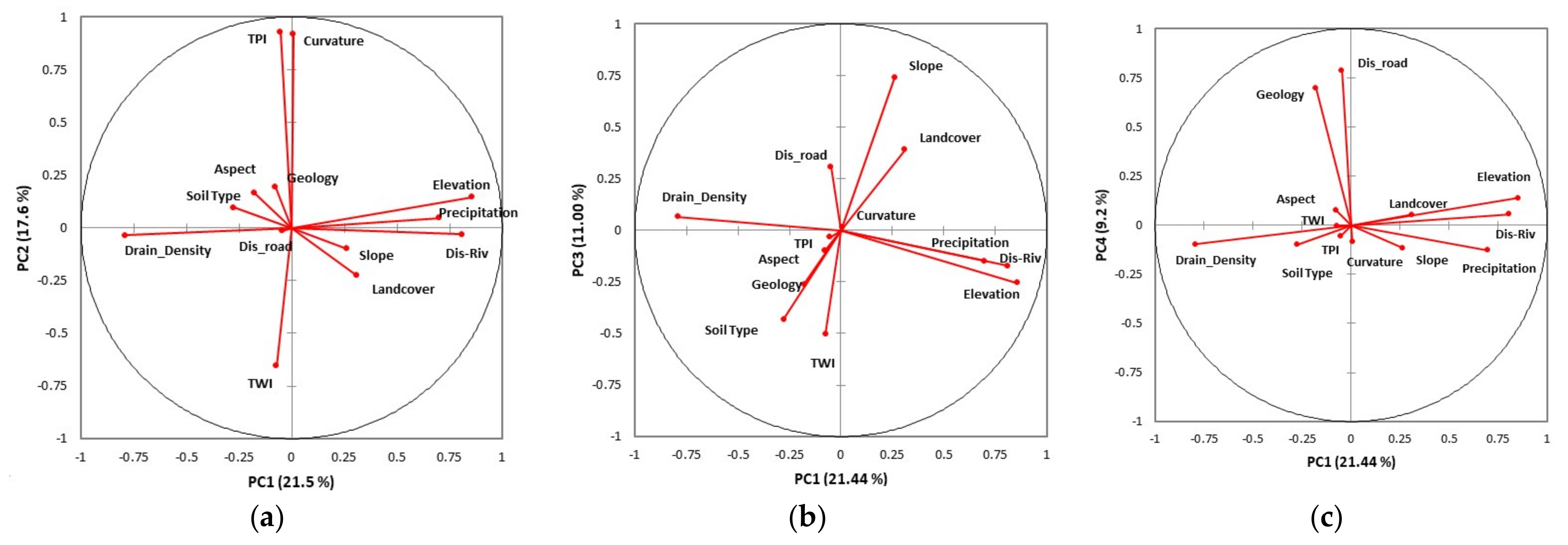
2.3.1. Principal Component Analysis

A principal component analysis (PCA) was performed by diagonalization of the correlation matrix in order to identify and rank the different sources of variability within the identified gully points. The principal components are linear combinations of the 13 parameters and thus behave as macro-parameters. They are orthogonal to each other and therefore represent independent sources of variability, i.e., independent associated processes. Taking into account the main PCs makes it possible to concentrate the information in a reduced number of factorial axes while losing a minimum of the information contained in the dataset, which constitutes a dimensional reduction of the data hyper-space [45,46,47,48].

2.3.2. Gully Susceptibility Prediction

Gully occurrence prediction was performed using the gully and non-gully points as the dependent variables and the 13 parameters as independent variables and input data. We used four machine learning algorithms, multivariate discriminant analysis (MDA), logistic regression (LR), classification and regression tree (CART), and random forest (RF), for susceptibility modeling. A ratio of 80 to 20 of data was considered for training and testing the models, respectively. The models used are described as follows:

• Multivariate discriminant analysis (MDA) is a conventionally and widely used tool to study groups of observations that may have different characteristics [45]. MDA has shown good performance for classification and modeling in several hydrological and hydrochemical studies [14,46,48,49,50,51]. MDA is a generalization of Fisher’s linear discriminant, a method used in statistics, pattern recognition, and machine learning to find a linear combination of features that characterizes or separates two or more classes of objects or events. The resulting combination, called discriminant functions, may be used as a linear classifier, or, more commonly, to reduce the dimensionality between before and after the classification. The discriminant function can be defined as follows:

  F = V₁W₁ + V₂W₂… + V_nW_n,

  (1)

  where F, V₁, and W₁ represent the discriminant score, the independent variables, and the discriminant weights, respectively.
• Logistic regression (LR) is a statistical model that can describe the relationship between the probability of a binary response variable and a set of corresponding explanatory variables. It is a generalized linear model using a logistic function as a link function [52,53]. In this study, the logistic regression algorithm has been used to predict the probability of gully erosion to develop (value = 1) or not (value = 0) based on the optimization of the regression coefficients and using a logit natural logarithms model. This result always varies between 0 and 1. A threshold is selected, above which a gully is likely to develop.
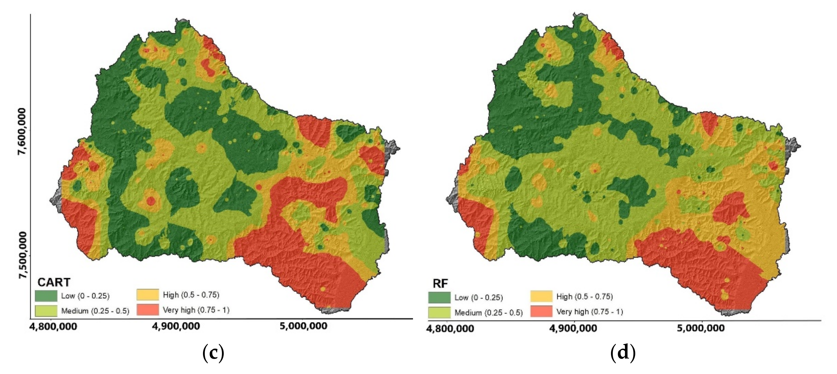
• Classification and regression tree (CART) is an effective decision tree-based algorithm and has proven to be powerful technique for handling classification problems. The CART generates a sequence of sub-trees for classification problems by growing a large tree instead of using stopping rules. Therefore, it is able to construct complex trees for solving complicated problems with large datasets. CART has been widely used in many studies of natural hazards such as landslides, subsidence, urban flooding, etc. [11,19,20,52]. Here, it is be applied to the prediction of gully development following a four-step procedure: (1) building the tree, (2) stopping the building of the tree, (3) pruning the tree, and (4) selecting the optimal tree for classifying gully or non-gully classes [19,54]. For this method, we also deployed the Gini index method to create binary divisions with a maximum tree depth of 4.
• Random forest is a method for learning sets of regressions and classifications based on the construction, at the time of testing, of many uncorrelated decision trees [55], using the Gini index of impurities [20,56]. The RF model uses bootstrap sampling, to be implemented in the evaluation, which allows another unused subset, also called the out-of-bag data (OOB), to be used for validation. Therefore, for the construction of the RF model, several tests were performed to find the best number of trees from 40 to 200 to obtain the best result. For this study, the OOB error is minimal for a number of 60 in the prediction for a given point to belong to the gully class or not. The final result is the class selected by most trees.

2.3.3. Validation, Performance Metrics and Evaluation Criteria

Validation techniques are valuable tools used in predictive modeling and machine learning to assess the consistency of results [21,28,57]. Even when prediction, variable selection, or model selection are not the focus, validation can help to assess the generalizability and reliability of results. The Hold-Out procedure is the most widely used technique in the validation of machine learning models [58,59]. It is based on dividing the database into two non-overlapping parts used for training and testing [60]. In this study, we used the Repeated Hold-Out method [61]. For 10 successive times, the data were randomly partitioned into 80% for training and 20% for testing. For each split, the four machine learning algorithms were applied on the training set and validated on the testing set. The average performance for each model was then computed using the arithmetic mean Equation (1):

$$\overline{P}=\frac{1}{K} {\displaystyle {\sum }_{i=1}^K}{P}_i,$$

(2)

where $\overline{P}$denotes the average value of a performance metric (it can be the total accuracy of the model or another metric), K denotes the number splits (where K = 10), and $P_i$ is the result of the performance metric of each split.

To ensure a proper evaluation of the modeling performance of the four machine learning models, we used four types of classification results provided by the confusion matrix, namely, accuracy (ACC; Equation (2)), sensitivity (SST; Equation (3)), specificity (SPF; Equation (4)), and precision (PRC; Equation (4)) [11,62]. In general, the higher the ACC, SST, SPF, and PRC values, the better the performance of the models.

$$\mathrm{ACC}=\frac{\mathrm{TP}+\mathrm{TN}}{\mathrm{TP}+\mathrm{TN}+\mathrm{FN}+\mathrm{FP}}$$

(3)

$$\mathrm{SST}=\frac{\mathrm{TP}}{\mathrm{TP}+\mathrm{FN}}$$

(4)

$$\mathrm{SPF}=\frac{\mathrm{TN}}{\mathrm{TN}+\mathrm{FP}}$$

(5)

$$\mathrm{PRC}=\frac{\mathrm{TP}}{\mathrm{TP}+\mathrm{FP}}$$

(6)

where TP, TN, FP, and FN are true positive, true negative, false positive, and false negative, respectively.

Model evaluation was also performed using the Receiver Operating Characteristic curve (ROC) statistic, which is a common criterion for evaluating spatial modeling performance [11]. The ROC curve value represents the probability that a test point is accurately differentiated from a random point in the predetermined context of the study area. For ROC curve values ranging from 0.5 to 0.6, 0.6 to 0.7, 0.7 to 0.8, 0.8 to 0.9, and 0.9 to 1, models are classified as poor, fair, good, very good, and excellent, respectively.

2.3.4. Contribution Analysis of Parameters

A Jackknife test was used to evaluate the contribution rates of the different parameters for each model of gully erosion susceptibility [63,64,65]. The main approach of this procedure is to leave out a predictor and examine the amount of bias or loss of information created by removing that predictor in the estimation model. The percentage decrease in overall accuracy (DACC) was used to examine the sensitivity of each indicator.

$${\mathrm{DACC}}_i=\frac{{\mathrm{ACC}}_{\mathrm{All}}-{\mathrm{ACC}}_i}{{\mathrm{ACC}}_{\mathrm{ALL}}}\times 100,$$

(7)

where ACC_all is the calculated value of the overall accuracy of the model using all parameters. ACC_i denotes the ACC value of the model when indicator i is removed from the input dataset, and DACC_i is the corresponding percentage decrease in ACC.

3. Results

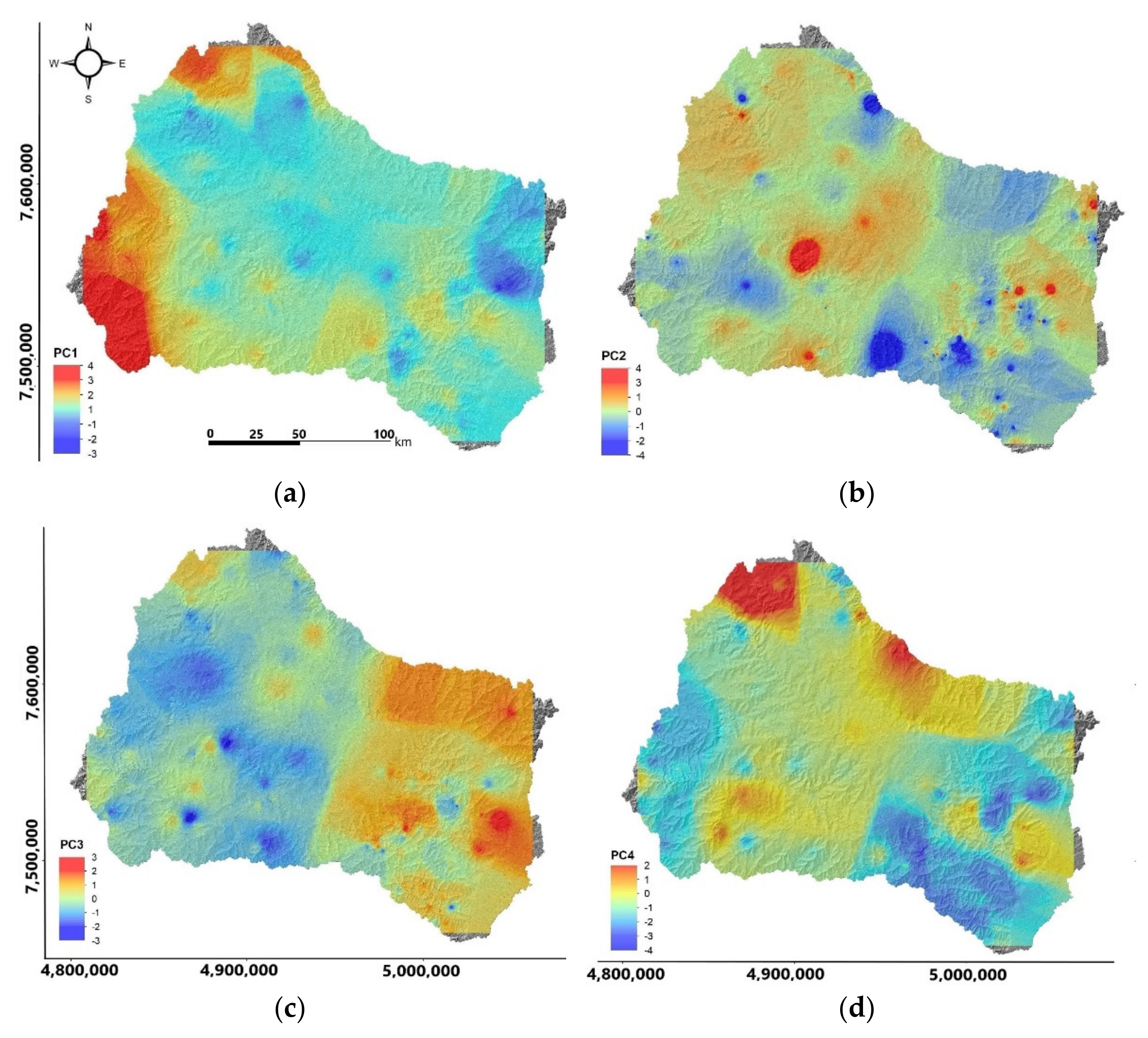
3.1. Principal Component Analysis and Distribution of PCs

The principal component analysis performed on the gully points showed that the first four principal components carried 62% of the information (

Table 2. Eigenvalues and percentage of variance explained by the first four principal components.

	PC1	PC2	PC3	PC4
Eigenvalue	2.8	2.3	1.4	1.2
Variance explained (%)	21.5	17.6	11	9.2
Cumulative %	21.5	39.1	50.1	59.3

). PC1 alone explained 21.5% of the variance, showing high positive correlations with altitude, distance to river, and rainfall (Figure 5a) and a negative correlation with drainage density. PC2 explains 17.6% of the variance, showing high positive correlations with TPI and curvature and a negative correlation with TWI (Figure 5a). PC3 explained 11% of the variance, had positive correlations with slope and land cover, and negative correlations with TWI and soil type (Figure 5b). PC3 explained 9.2% of the variance, showing high positive correlations with geology and distance to road (Figure 5c).

The distribution of these four PCs is shown in Figure 6. Areas with negative values on PC1 (blue color) were along the drainage network and downstream of the basin. They corresponded to areas of high drainage density. The intermediate values (yellow color) occurred on the relatively high slopes of the first-order tributaries of the drainage network, and they indicated slightly high relief conditions with rather high precipitation. The highest positive values (orange and red color) were at the headwaters of the basin where precipitation is highest. The high and negative values on PC2, which reflected high values of TWI, were concentrated in the downstream part of the basin, with some spots located in the upstream part, indicating high soil moisture and high drainage capacities. The positive values of PC2 that reflected high values of IPT and curvature were mostly located in the upstream and central part of the basin, i.e., an area characterized by rather high hills. PC3 explained a significant part of the variability in the gullying conditions that combined the parameters slope, land cover, soil moisture (TWI), and soil type. The high positive PC3 values located mainly in the downstream regions of the basin reflected high slope, land cover dominated by pasture, and coarse-textured red oxisols–ultisols catena. Negative PC3 values combined gullies developing under conditions of high drainage capacity and soil moisture (High TWI), land use dominated by field crops (sorghum–cotton–corn crops rotations, secondarily sugarcane), and finer-textured, strongly micro-aggregated purple oxisols–ultisols catena (Figure 6d). PC4 shows a very similar distribution to the geological formations (Figure 6c). The high values are associated with the Sera Geral formation in the upstream part of the study area, and secondarily with high distances to road infrastructure. The low values are consistent with the Caiuá fine sandstone formations and very short distance to road.

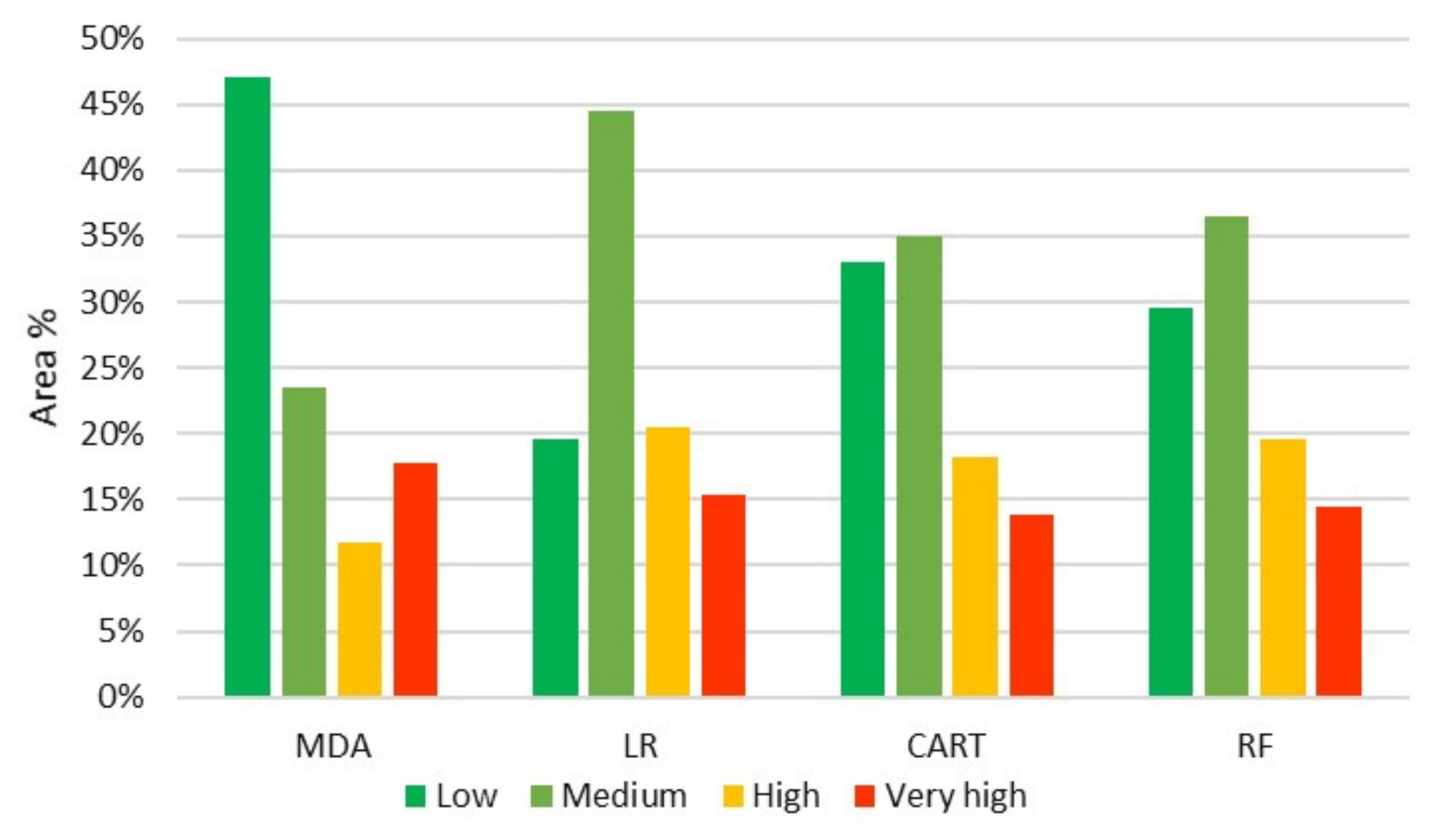
3.2. Machine Learning

Table 3. Predictive capability of models using training data.

Statistical Index	MDA	LR	CART	RF
Accuracy (%)	78.47	77.62	82.81	86.09
Specificity (%)	74.36	75.91	88.09	85.40
Sensitivity (%)	82.47	79.33	77.57	86.79
Precision (%)	76.78	77.05	86.76	85.45

and

Table 4. Predictive capability of models using test data.

Statistical Index	MDA	LR	CART	RF
Accuracy (%)	72.50	78.54	84.38	89.83
Specificity (%)	71.42	81.39	80.61	90.24
Sensitivity (%)	73.33	75.67	88.61	88.46
Precision (%)	67.56	77.78	81.39	86.61

show the validation results of the four machine learning algorithms for training and test data, respectively. All statistical indices (accuracy, specificity, sensitivity, and precision) are high, whatever the model, for both training and test data (from 71% to 90%).

For the training data, the performance of the procedures could be ranked as follows: accuracy (RF > CART > LR > MDA), specificity (RF > CART > LR > MDA), and sensitivity and precision RF > MDA > LR > CART). The results obtained on the test data showed that the RF algorithm had the best results compared to the others.

Table 5. Models’ evaluation using the Receiver Operating Characteristic (ROC) curve statistic.

	MDA	LR	CART	RF
ROC Curve	0.850	0.861	0.920	0.931

shows the overall performance of the four models using the ROC curve index, with all values above 0.8. From these data, it can be concluded that all of the models perform very well, although the RF algorithm showed the best spatial predictive ability for gullies (RF > CART > LR > MDA).

The gully susceptibility maps produced by the four models are shown in Figure 7. Susceptibility was divided into four classes using the natural break method [66,67]: low (0–0.25), medium (0.25–0.5), high (0.5–0.75), and very high (0.75–1). The four models used led to very close results and a very similar distribution of susceptibility prediction. The areas of high and very high susceptibility were located in the eastern third of the basin as well as on the extreme western and northern edges. The areas affected by high and very high susceptibility were quite similar: for RF, 19.6% and 14.4%; for CART, 18.3% and 14%; for MDA, 19% and 14%; and for LR, 20.4% and 15.5%, respectively (Figure 8).

3.3. Contribution of Factors to Susceptibility Mapping

Assessing the importance of the explanatory variables provides a better understanding of the gully erosion problem, and it is a practical means for environmental managers to allocate and plan adequate resources for natural resource management [16,20]. While the susceptibility areas and their distributions were similar, the contributing parameters differed between models. In the case of the MDA model, the order of the top four parameters that contribute most to the model was geology > distance to road network > distance to river network > slope (Figure 9a). For the LR model, the contribution was geology > distance to river network > distance to road network > slope (Figure 9b). The most influential parameters according to the CART model were land cover > distance to road network > precipitation > distance to the river network (Figure 9c). Finally, the RF model identified elevation > land cover > distance to the river network > geology > precipitation (Figure 9d). In all four models, the TPI and TWI parameters did not contribute significantly to the susceptibility modeling.

4. Discussion

4.1. Processes Associated with the Diversity of Gully Conditions

The analysis of the main factors associated with the presence of gullies highlights two main situations favoring the development of this form of erosion in the study area. The first situation is discriminated by positive values on the factorial axes PC1 and PC2, and is mainly developed in the upstream part of the basin, in the western, northwestern, and southwestern sectors. The altitudes are higher; the precipitation more important. These two parameters showed major influence on gully development. The positive correlations of the parameters with PC1 and PC2 teach us that these gullies develop rather far from the hydrographic network, i.e., their development is barely influenced by this drainage network. The erosion marks more particularly the high parts of the slopes with concave profile, reflected by the parameter of slope curvature and the TPI index. Under these conditions, accelerated flow and high runoff promote surface erosion [13,68]. Numerous erosion rills can be observed leading to deep gullies. In Figure 10, the situations from 2002 to 2021 show the progressive development of an erosion ripple to a gully. This is a genetic relationship often described in many parts of the world [69,70]. When erosion channels appear on the soil surface, runoff concentrates, scours, carries soil particles, and rill erosion develops. Once formed, erosion increases rapidly, and the morphology of the slope is constantly modified. Water depth, flow velocity, and erosive force increase as the gully develops. If the water table is reached, the mode of erosion changes drastically; the gully profile, initially V-shaped (ravina-type gullies), turns into U-shaped (voçoroca-type gullies); and a rapid upstream progression can be observed, mobilizing considerable amounts of material [71]. The second case is characterized by negative values on the PC1 and PC2 axes. These gullies develop at lower elevations, close to the drainage network, under conditions of high drainage density and on low slopes. The negative correlation with TWI in PC2 reflects an influence of areas prone to water accumulation, i.e., high contributing surface area [68]. Areas with high drainage density, which is generally determined by lithology, vegetation cover, and landform properties [46,72], reflect conditions of high runoff relative to infiltration, favoring surface runoff erosion. These are mainly the conditions observed in the central and downstream part of the Ivinhema basin. In contrast to the previous case, erosion rills are absent, and gullying starts at low points near the drainage system (Figure 11), i.e., areas of the landscape where the water table is close to the topsoil, and leading mainly to voçoroca-type gullies. These areas are generally valorized with pasture. These two above-mentioned cases represent 39% of the variance on the whole dataset and are clearly discriminated by positive or negative coordinates on PC1 and PC2, i.e., the processes responsible for this diversity are distinct.

The first significant contribution of soil type and land cover is observed on the PC3 factorial axis in correlation with slope and TWI. Such an association of parameters suggests that PC3 reflects soil moisture conditions, its infiltration, and surface runoff potential [72]. The distribution of PC3 values clearly divides the basin into two parts. To the east, the gullies are associated with slopes in the pasture zone. These characteristics are in agreement with the conclusions of Castro and Queiroz Neto [37], who mention that the paths created by the trampling of livestock converging on water tanks, as observed in Figure 12, or plot corridors favor runoff and cause gullying. In addition, several detailed soil studies carried out on sandstone formations, mainly used for livestock production, have shown the development of a Bt horizon progressing up the slopes, shifting the drainage from vertical to lateral and sub-surface, favoring a piping phenomenon that eventually leads to the formation of gullies [73]. The development and functioning of typical soil covers, representative of large regions, constitute crucial information, much more useful than a soil map, and should be taken into consideration in future multiparameter analysis of erosion patterns [74,75,76]. In the western part of the basin, gullies assigned to negative values on PC3 are associated with the presence of field crops and high TWI indexes. Sorghum–cotton–maize crop rotations require intense and continuous mechanization while being developed, from seeding to harvest time, weakening the surface condition of the soil, generating a deep compacted layer that causes decreased infiltration of rainwater, thereby increasing surface runoff, and favoring linear erosion likely to evolve into gullies. Thus, PC3 represents the relationship between exploitation and water erosion in areas that are not suitable for such activities [37,77,78,79].

The influence of human activity only appears on the factorial axis PC4, through the parameter of distance to the road network, and itself coupled with the geology. This factorial axis is responsible for 9.2% of the variance, which suggests that the coupling between the lithology and human activity influences the development of gullies, but to a much lesser extent than the factors of relief, climate, drainage network, and land characteristics. The strong positive correlations of PC4 with the geology parameter and the distance to the road network suggest that the influence of human activity on the development of gullies depends on the lithology of the area. This PC4 reflects the gullies developed on the Caiuá sandstone formations (i.e., in the southeastern region of the Ivinhema basin) and near the road network. Thus, in this area, it appears crucial to be vigilant in the construction of the road network and the trails of access to the plots, likely to activate the formation and development of gullies (Figure 13). If this factor does not appear as a major factor in our analysis, it is largely due to the prevailing rurality and low population density (about 0.5 inhabitants per km²) in our study area. The information related to this specific context is somewhat buried in the larger amount of information related to the whole study area. Such gullies are located on the periphery of urban areas where the pressure on the environment is stronger. These results agree with those of Guerra et al. [80], who mention that irregular habitat and inadequate land cover on a lithology of low erosion resistivity play major roles in the formation and evolution of gullies. The coordinates of the parameters on PC4 highlight that the gullies that are not influenced by human activity are located to the west and northwest of the study area, represented by the negative values of PC4. In this sector, the urban areas are rare and modest in size, but the analysis of satellite imagery reveals traces of convergence of the cattle towards the artificial water points (small dams locally called “Açudes”). These pathways can give rise to erosion rills likely to evolve into ravina-type and voçoroca-type gullies, as shown in the satellite images (1) and (3) in Figure 2 and Figure 12. This is a parameter of anthropic pressure on the environment that has not been taken into account in our study.

4.2. A Multi Parameter Contribution to Gully Formation

The four models used to map gully erosion susceptibility performed well. The ROC curve statistic indicates that all models have excellent performance (0.850–0.931) and exhibit high capability (ROC curve > 0.8) in predicting gully erosion susceptibility. This level of performance is in line with previous work conducted on gully erosion in other regions of the world and reflects the strength of the machine learning models adopted and the relevance of the geo-environmental parameters chosen for the susceptibility mapping [10,21,22].

However, the RF algorithm shows the best performance, confirming the advantage of decision tree-based models over linear models (Table 3 and Table 4). These results are in agreement with several studies that aimed at the application of machine learning approaches for susceptibility mapping of different types of natural hazards, such as landslide, soil subsidence, and flooding [11,52,81,82,83,84]. In a recent publication on gully erosion, Lana et al. [25] found that the tree-based ensemble outperformed other algorithms used in the development of gully erosion predictive models on a regional scale. These authors also found that decision tree models (especially the RF algorithm) often outperform linear models, being able to meet statistical assumptions such as independence and statistical distributions of variables. These models can detect complex non-linear relationships, which is not the case with linear approaches [20,85,86,87]. However, although the RF algorithm is accurate and efficient, it is known to compromise interpretability for discrimination efficiency [88,89,90], a major constraint that limits the identification of the processes behind the phenomenon under study [91,92,93].

Parameter contribution analysis is of practical interest to environmental managers in charge of allocating and planning funds, often limited, for natural resource management [20,94]. In previous studies related to other types of natural hazards (snow avalanches and landslides), this analysis usually highlights the dominance of one or two major factors in the susceptibility to the studied hazard, with contribution proportions ranging from 15% to 50% or even 80% [14,15,20,94]. In our study, for the best performing RF algorithm, the factor contribution analysis highlighted that elevation, land cover, geology, and precipitation are the factors that most condition the development of gully erosion. Several studies have described the strong contribution of the latter parameters in conditioning gully erosion on both local and regional scales [10,21,22]. Secondary factors were distance to the rivers and to roads, slope, and drainage density. The other algorithms rely on these same factors for mapping. However, the low DACC values, less than 7%, emphasize that gully formation is not governed by one or two major factors, and that this type of erosion is complex in nature. On this point, despite their mathematical distinctions, both machine learning and PCA agree on the complexity of the factors involved in the development of gullies.

The study reveals the diversity of situations in which gullying develops in the study area, as well as the associations of spatially variable factors, i.e., a strong complexity in the determinism of erosion. Therefore, for a local application, the susceptibility maps are all quite similar, but must be used with knowledge of this diversity, depending on the specific situation on a case by case basis. In general, compared to lower flat areas, high elevation areas have a relatively high potential for gully erosion under conditions of high rainfall and runoff. Higher relief accelerates surface runoff, paving the way for soil erosion [22,35]. Land cover and land use are also known to play important roles in gully formation. In Brazil, extensive rotational cropping, with tillage practices that increase surface runoff, is the most susceptible to gully erosion [73]. The contribution of geology to susceptibility modeling has been widely recognized [22,35,67], and it must be kept in mind that the geology parameter shows a high contribution in the four models. Areas of very high susceptibility are all located on the Caiuá formation. Castro and Queiroz Neto [37] mentioned the presence of more than 9000 large voçoroca-type gullies in the Parana sedimentary basin, 80% of which were developed on ultisols derived from the fine sandstone formations, particularly from the Caiuá and Baurú groups. Anthropogenic action, often decried as a cause of gully development, appears only as a contributing factor in addition to other natural features that favor gullying. However, the largest voçoroca-type gullies recorded in the study area are in the peri-urban areas of the Caiuá formation near the drainage network (Figure 11).

5. Conclusions

In this work, we studied the different factors controlling the formation and development of gully erosion and established susceptibility maps in the Rio Ivinhema basin in the state of South Mato Grosso, Brazil. The database constructed on gully erosion and 13 geo-environmental factors was analyzed by a multifactorial statistical approach (principal component analysis (PCA)) and by machine learning with four different algorithms, multivariate discriminant analysis (MDA), logistic regression (LR), classification and regression tree (CART), and random forest (RF). This type of analysis highlights the existence of distinct major processes (in this case, two major processes) that take place in different sectors of the study area. In the western part of the basin, i.e., in the upstream region, the gullies are accompanied by rill erosion and do not develop near the drainage network. In the center and east of the basin, on the other hand, large gullies (long, wide, and deep) develop near the drainage system. Human activity, represented by the parameter of distance to the road network, contributes significantly to the formation of gullies, but only under specific geological conditions, mainly on the sandstones of the Caiuá formation. The influence of human activity also seems to be related to the construction of small earth dams for cattle feeding, mainly in the western part of the basin, but this parameter was not considered and quantified in the study. Human activity is also related to rotary crops, which interfere intensively with the soil. The study shows that this kind of approach should be carried out in parallel with studies of the organization of soil cover along broadly representative catena, including the path of water. Such studies would help considerably in the interpretation of our results. All four models performed well in mapping gully susceptibility (ROC curve > 0.8), giving very similar results, although slightly better in the case of the random forest algorithm. Areas of high to very high susceptibility (29% < area < 35% of the study area) involve regions with high relief and precipitation, short distance to rivers and roads, and sandstone lithology, mainly the Caiuá formation. Analysis of the contribution of the descriptor parameters selected for the study shows that susceptibility to gullying is not governed primarily by a single factor, but by the contribution of several factors that reflect several complex spatially distributed processes. In a context of risk reduction and sustainable land management, the results of the study should help the authorities and stakeholders concerned to make decisions, but by considering the processes involved on a case-by-case basis for each area to be developed.

References

1. Martineli Costa, F.; Bacellar, L.A.T. Analysis of the influence of gully erosion in the flow pattern of catchment streams, Southeastern Brazil. CATENA 2007, 69, 230–238. [Google Scholar] [CrossRef]
2. Castillo, C.; Gómez, J.A. A century of gully erosion research: Urgency, complexity and study approaches. Earth-Sci. Rev. 2016, 160, 300–319. [Google Scholar] [CrossRef]
3. De Bacellar, L.A.P.; Coelho Netto, A.L.; Lacerda, W.A. Controlling factors of gullying in the Maracujá Catchment, southeastern Brazil. Earth Surf. Process. Landf. 2005, 30, 1369–1385. [Google Scholar] [CrossRef]
4. Guerra, A.J.T.; Fullen, M.A.; Bezerra, J.F.; Jorge, M.C.O. Gully Erosion and Land Degradation in Brazil: A Case Study from São Luís Municipality, Maranhão State. In Ravine Lands: Greening for Livelihood and Environmental Security; Dagar, J.C., Singh, A.K., Eds.; Springer: Singapore, 2018; pp. 195–216. ISBN 978-981-10-8043-2. [Google Scholar]
5. Tricart, J. Ecodinâmica; Instituto Brasileiro de Geografia e Estatística: Rio de Janeiro, Brazil, 1977. [Google Scholar]
6. Christofoletti, A. Análise de Sistemas em Geografia: Introdução; Hucitec/Edusp: São Paulo, Brazil, 1979. [Google Scholar]
7. Ross, J. Análise empírica da fragilidade dos ambientes naturais e antrópizados. Rev. Dep. Geogr. São Paulo 1994, 8, 63–74. [Google Scholar] [CrossRef] [Green Version]
8. Crepani, E.; de Medeiros, J.S.; Hernandez Filho, P.; Florenzano, T.G.; Duarte, V.; Barbosa, C.C.F. Sensoriamento Remoto e Geoprocessamento Aplicados ao Zoneamento Ecológico-Econômico e ao Ordenamento Territorial; Inpe: São José dos Campos, Brazil, 2001. [Google Scholar]
9. Conoscenti, C.; Angileri, S.; Cappadonia, C.; Rotigliano, E.; Agnesi, V.; Märker, M. Gully erosion susceptibility assessment by means of GIS-based logistic regression: A case of Sicily (Italy). Geomorphology 2014, 204, 399–411. [Google Scholar] [CrossRef] [Green Version]
10. Arabameri, A.; Pradhan, B.; Rezaei, K.; Conoscenti, C. Gully erosion susceptibility mapping using GIS-based multi-criteria decision analysis techniques. CATENA 2019, 180, 282–297. [Google Scholar] [CrossRef]
11. Bouramtane, T.; Kacimi, I.; Bouramtane, K.; Aziz, M.; Abraham, S.; Omari, K.; Valles, V.; Leblanc, M.; Kassou, N.; El Beqqali, O.; et al. Multivariate analysis and machine learning approach for mapping the variability and vulnerability of urban flooding: The case of Tangier city, Morocco. Hydrology 2021, 8, 182. [Google Scholar] [CrossRef]
12. Tiouiouine, A.; Jabrane, M.; Kacimi, I.; Morarech, M.; Bouramtane, T.; Bahaj, T.; Yameogo, S.; Rezende-Filho, A.T.; Dassonville, F.; Moulin, M.; et al. Determining the relevant scale to analyze the quality of regional groundwater resources while combining groundwater bodies, physicochemical and biological databases in southeastern france. Water 2020, 12, 3476. [Google Scholar] [CrossRef]
13. Chang, K.-T.; Merghadi, A.; Yunus, A.P.; Pham, B.T.; Dou, J. Evaluating scale effects of topographic variables in landslide susceptibility models using GIS-based machine learning techniques. Sci. Rep. 2019, 9, 12296. [Google Scholar] [CrossRef] [Green Version]
14. Choubin, B.; Borji, M.; Mosavi, A.; Sajedi-Hosseini, F.; Singh, V.P.; Shamshirband, S. Snow avalanche hazard prediction using machine learning methods. J. Hydrol. 2019, 577, 123929. [Google Scholar] [CrossRef]
15. Choubin, B.; Moradi, E.; Golshan, M.; Adamowski, J.; Sajedi-Hosseini, F.; Mosavi, A. An ensemble prediction of flood susceptibility using multivariate discriminant analysis, classification and regression trees, and support vector machines. Sci. Total Environ. 2019, 651, 2087–2096. [Google Scholar] [CrossRef] [PubMed]
16. Darabi, H.; Choubin, B.; Rahmati, O.; Torabi Haghighi, A.; Pradhan, B.; Kløve, B. Urban flood risk mapping using the GARP and QUEST models: A comparative study of machine learning techniques. J. Hydrol. 2019, 569, 142–154. [Google Scholar] [CrossRef]
17. Dodangeh, E.; Panahi, M.; Rezaie, F.; Lee, S.; Tien Bui, D.; Lee, C.-W.; Pradhan, B. Novel hybrid intelligence models for flood-susceptibility prediction: Meta optimization of the GMDH and SVR models with the genetic algorithm and harmony search. J. Hydrol. 2020, 590, 125423. [Google Scholar] [CrossRef]
18. Merghadi, A.; Yunus, A.P.; Dou, J.; Whiteley, J.; ThaiPham, B.; Bui, D.T.; Avtar, R.; Abderrahmane, B. Machine learning methods for landslide susceptibility studies: A comparative overview of algorithm performance. Earth-Sci. Rev. 2020, 207, 103225. [Google Scholar] [CrossRef]
19. Pham, B.T.; Prakash, I.; Tien Bui, D. Spatial prediction of landslides using a hybrid machine learning approach based on Random Subspace and Classification and Regression Trees. Geomorphology 2018, 303, 256–270. [Google Scholar] [CrossRef]
20. Rahmati, O.; Falah, F.; Naghibi, S.A.; Biggs, T.; Soltani, M.; Deo, R.C.; Cerdà, A.; Mohammadi, F.; Tien Bui, D. Land subsidence modelling using tree-based machine learning algorithms. Sci. Total Environ. 2019, 672, 239–252. [Google Scholar] [CrossRef] [PubMed]
21. Garosi, Y.; Sheklabadi, M.; Conoscenti, C.; Pourghasemi, H.R.; Van Oost, K. Assessing the performance of GIS- based machine learning models with different accuracy measures for determining susceptibility to gully erosion. Sci. Total Environ. 2019, 664, 1117–1132. [Google Scholar] [CrossRef]
22. Pourghasemi, H.R.; Sadhasivam, N.; Kariminejad, N.; Collins, A.L. Gully erosion spatial modelling: Role of machine learning algorithms in selection of the best controlling factors and modelling process. Geosci. Front. 2020, 11, 2207–2219. [Google Scholar] [CrossRef]
23. De Freitas Sampaio, L.; Crestana, S.; Rodrigues, V.G.S. Study of Gully Erosion in South Minas Gerais (Brazil) Using Fractal and Multifractal Analysis. In Proceedings of the IAEG/AEG Annual Meeting Proceedings, San Francisco, CA, USA, 26 August 2018; Shakoor, A., Cato, K., Eds.; Springer International Publishing: Cham, Switzerland, 2019; Volume 6, pp. 217–222. [Google Scholar]
24. Real, L.S.C.; Crestana, S.; Ferreira, R.R.M.; Rodrigues, V.G.S. Evaluation of gully development over several years using GIS and fractal analysis: A case study of the Palmital watershed, Minas Gerais (Brazil). Environ. Monit. Assess. 2020, 192, 434. [Google Scholar] [CrossRef]
25. Lana, J.C.; de Tarso Amorim Castro, P.; Lana, C.E. Assessing gully erosion susceptibility and its conditioning factors in southeastern Brazil using machine learning algorithms and bivariate statistical methods: A regional approach. Geomorphology 2022, 402, 108159. [Google Scholar] [CrossRef]
26. Milani, E.; Rangel, H.; Bueno, G.; Stica, J.; Winter, W.; Caixeta, J.; Neto, O. Bacias Sedimentares Brasileiras-Cartas Estratigraficas. Bol. Geociênc. Da Petrobras 2007, 15, 183–205. [Google Scholar]
27. Fernandes, L.A.; Coimbra, A.M. O grupo caiuá (Ks): Revisão estratigráfica e contexto deposicional. Rev. Bras. Geociênc. 1994, 24, 164–176. [Google Scholar] [CrossRef]
28. Hembram, T.K.; Saha, S.; Pradhan, B.; Maulud, K.N.A.; Alamri, A.M. Robustness analysis of machine learning classifiers in predicting spatial gully erosion susceptibility with altered training samples. Geomat. Nat. Hazards Risk 2021, 12, 794–828. [Google Scholar] [CrossRef]
29. Roy, J.; Saha, S. Integration of artificial intelligence with meta classifiers for the gully erosion susceptibility assessment in Hinglo river basin, Eastern India. Adv. Space Res. 2021, 67, 316–333. [Google Scholar] [CrossRef]
30. Zhang, P.; Yao, W.; Liu, G.; Xiao, P. Experimental study on soil erosion prediction model of loess slope based on rill morphology. CATENA 2019, 173, 424–432. [Google Scholar] [CrossRef]
31. Tsangaratos, P.; Ilia, I. Comparison of a logistic regression and Naïve Bayes classifier in landslide susceptibility assessments: The influence of models complexity and training dataset size. CATENA 2016, 145, 164–179. [Google Scholar] [CrossRef]
32. Hembram, T.K.; Paul, G.C.; Saha, S. Comparative Analysis between Morphometry and Geo-Environmental Factor Based Soil Erosion Risk Assessment Using Weight of Evidence Model: A Study on Jainti River Basin, Eastern India. Environ. Process. 2019, 6, 883–913. [Google Scholar] [CrossRef]
33. Jaafari, A.; Najafi, A.; Pourghasemi, H.R.; Rezaeian, J.; Sattarian, A. GIS-based frequency ratio and index of entropy models for landslide susceptibility assessment in the Caspian forest, northern Iran. Int. J. Environ. Sci. Technol. 2014, 11, 909–926. [Google Scholar] [CrossRef] [Green Version]
34. Conforti, M.; Aucelli, P.P.C.; Robustelli, G.; Scarciglia, F. Geomorphology and GIS analysis for mapping gully erosion susceptibility in the Turbolo stream catchment (Northern Calabria, Italy). Nat. Hazards 2011, 56, 881–898. [Google Scholar] [CrossRef]
35. Shit, P.K.; Nandi, A.S.; Bhunia, G.S. Soil erosion risk mapping using RUSLE model on jhargram sub-division at West Bengal in India. Model. Earth Syst. Environ. 2015, 1, 28. [Google Scholar] [CrossRef] [Green Version]
36. Kopecký, M.; Macek, M.; Wild, J. Topographic Wetness Index calculation guidelines based on measured soil moisture and plant species composition. Sci. Total Environ. 2021, 757, 143785. [Google Scholar] [CrossRef]
37. De Castro, S.S.; de Queiroz Neto, J.P. Soil Erosion in Brazil from Coffee to the Present-day Soy Bean Production. In Natural Hazards and Human-Exacerbated Disasters in Latin America; Latrubesse, E.M., Ed.; Developments in Earth Surface Processes; Elsevier: Amsterdam, The Netherlands, 2009; Volume 13, pp. 195–221. [Google Scholar]
38. CRPM Mapa Geodiversidade do Estado do Mato Grosso do Sul. Available online: https://rigeo.cprm.gov.br/handle/doc/14703 (accessed on 20 January 2022).
39. Cao, L.; Wang, Y.; Liu, C. Study of unpaved road surface erosion based on terrestrial laser scanning. CATENA 2021, 199, 105091. [Google Scholar] [CrossRef]
40. Katz, H.A.; Daniels, J.M.; Ryan, S. Slope-area thresholds of road-induced gully erosion and consequent hillslope–channel interactions. Earth Surf. Process. Landf. 2014, 39, 285–295. [Google Scholar] [CrossRef]
41. Yu, W.; Zhao, L.; Fang, Q.; Hou, R. Contributions of runoff from paved farm roads to soil erosion in karst uplands under simulated rainfall conditions. CATENA 2021, 196, 104887. [Google Scholar] [CrossRef]
42. Zhang, Y.; Wang, Y.; Chen, Y.; Liang, F.; Liu, H. Assessment of future flash flood inundations in coastal regions under climate change scenarios—A case study of Hadahe River basin in northeastern China. Sci. Total Environ. 2019, 693, 133550. [Google Scholar] [CrossRef] [PubMed]
43. Defersha, M.B.; Melesse, A.M. Effect of rainfall intensity, slope and antecedent moisture content on sediment concentration and sediment enrichment ratio. CATENA 2012, 90, 47–52. [Google Scholar] [CrossRef]
44. Wu, X.; Wei, Y.; Wang, J.; Xia, J.; Cai, C.; Wei, Z. Effects of soil type and rainfall intensity on sheet erosion processes and sediment characteristics along the climatic gradient in central-south China. Sci. Total Environ. 2018, 621, 54–66. [Google Scholar] [CrossRef]
45. Bouramtane, T.; Yameogo, S.; Touzani, M.; Tiouiouine, A.; El Janati, M.; Ouardi, J.; Kacimi, I.; Valles, V.; Barbiero, L. Statistical approach of factors controlling drainage network patterns in arid areas. Application to the Eastern Anti Atlas (Morocco). J. Afr. Earth Sci. 2020, 162, 103707. [Google Scholar] [CrossRef]
46. Bouramtane, T.; Tiouiouine, A.; Kacimi, I.; Valles, V.; Talih, A.; Kassou, N.; Ouardi, J.; Saidi, A.; Morarech, M.; Yameogo, S.; et al. Drainage Network Patterns Determinism: A Comparison in Arid, Semi-Arid and Semi-Humid Area of Morocco Using Multifactorial Approach. Hydrology 2020, 7, 87. [Google Scholar] [CrossRef]
47. Rezende-Filho, A.T.; Valles, V.; Furian, S.; Oliveira, C.M.S.C.; Ouardi, J.; Barbiero, L. Impacts of lithological and anthropogenic factors affecting water chemistry in the upper Paraguay River Basin. J. Environ. Qual. 2015, 44, 1832–1842. [Google Scholar] [CrossRef]
48. Tiouiouine, A.; Yameogo, S.; Valles, V.; Barbiero, L.; Dassonville, F.; Moulin, M.; Bouramtane, T.; Bahaj, T.; Morarech, M.; Kacimi, I. Dimension Reduction and Analysis of a 10-Year Physicochemical and Biological Water Database Applied to Water Resources Intended for Human Consumption in the Provence-Alpes-Côte d’Azur Region, France. Water 2020, 12, 525. [Google Scholar] [CrossRef] [Green Version]
49. Anderson, R.H.; Farrar, D.B.; Thoms, S.R. Application of discriminant analysis with clustered data to determine anthropogenic metals contamination. Sci. Total Environ. 2009, 408, 50–56. [Google Scholar] [CrossRef] [PubMed]
50. Wilson, S.R.; Close, M.E.; Abraham, P. Applying linear discriminant analysis to predict groundwater redox conditions conducive to denitrification. J. Hydrol. 2018, 556, 611–624. [Google Scholar] [CrossRef]
51. Yameogo, S.; Nikiema, J.; Compaore, N.F.; Tiouiouine, A.; Rezende-filho, A.T.; Barbiero, L.; Valles, V. Discrimination de deux formations hydrogéologiques à partir de l’analyse mathématique des concentrations hydrochimiques d’eau souterraine en contexte sahélien de socle d’Afrique de l’Ouest: Cas de la commune de Markoye, Burkina Faso. Ann. L’université Joseph KI-ZERBO–Sér. C 2020, 17, 31–52. [Google Scholar]
52. Felicísimo, Á.M.; Cuartero, A.; Remondo, J.; Quirós, E. Mapping landslide susceptibility with logistic regression, multiple adaptive regression splines, classification and regression trees, and maximum entropy methods: A comparative study. Landslides 2013, 10, 175–189. [Google Scholar] [CrossRef]
53. Zhu, Z.; Lin, C.; Zhang, X.; Wang, K.; Xie, J.; Wei, S. Evaluation of geological risk and hydrocarbon favorability using logistic regression model with case study. Mar. Pet. Geol. 2018, 92, 65–77. [Google Scholar] [CrossRef]
54. Loh, W.-Y. Classification and regression trees. WIREs Data Min. Knowl. Discov. 2011, 1, 14–23. [Google Scholar] [CrossRef]
55. Breiman, L. Random Forests. Mach. Learn. 2001, 45, 5–32. [Google Scholar] [CrossRef] [Green Version]
56. Cutler, D.R.; Edwards, T.C., Jr.; Beard, K.H.; Cutler, A.; Hess, K.T.; Gibson, J.; Lawler, J.J. Random forests for classification in ecology. Ecology 2007, 88, 2783–2792. [Google Scholar] [CrossRef]
57. Shmueli, G. To Explain or to Predict? Stat. Sci. 2010, 25, 289–310. [Google Scholar] [CrossRef]
58. Monteiro, J.M.; Rao, A.; Shawe-Taylor, J.; Mourão-Miranda, J. A multiple hold-out framework for Sparse Partial Least Squares. J. Neurosci. Methods 2016, 271, 182–194. [Google Scholar] [CrossRef] [PubMed] [Green Version]
59. Pal, K.; Patel, B.V. Data Classification with k-fold Cross Validation and Holdout Accuracy Estimation Methods with 5 Different Machine Learning Techniques. In Proceedings of the 2020 Fourth International Conference on Computing Methodologies and Communication (ICCMC), Erode, India, 11–13 March 2020; pp. 83–87. [Google Scholar]
60. Yadav, S.; Shukla, S. Analysis of k-Fold Cross-Validation over Hold-Out Validation on Colossal Datasets for Quality Classification. In Proceedings of the 2016 IEEE 6th International Conference on Advanced Computing (IACC), Bhimavaram, India, 27–28 February 2016; pp. 78–83. [Google Scholar]
61. Tanner, E.M.; Bornehag, C.-G.; Gennings, C. Repeated holdout validation for weighted quantile sum regression. MethodsX 2019, 6, 2855–2860. [Google Scholar] [CrossRef]
62. Abraham, S.; Huynh, C.; Vu, H. Classification of Soils into Hydrologic Groups Using Machine Learning. Data 2020, 5, 2. [Google Scholar] [CrossRef] [Green Version]
63. Arabameri, A.; Chen, W.; Loche, M.; Zhao, X.; Li, Y.; Lombardo, L.; Cerda, A.; Pradhan, B.; Bui, D.T. Comparison of machine learning models for gully erosion susceptibility mapping. Geosci. Front. 2020, 11, 1609–1620. [Google Scholar] [CrossRef]
64. Moradi, E.; Abdolshahnejad, M.; Borji Hassangavyar, M.; Ghoohestani, G.; da Silva, A.M.; Khosravi, H.; Cerdà, A. Machine learning approach to predict susceptible growth regions of Moringa peregrina (Forssk). Ecol. Inform. 2021, 62, 101267. [Google Scholar] [CrossRef]
65. Park, N.-W. Using maximum entropy modeling for landslide susceptibility mapping with multiple geoenvironmental data sets. Environ. Earth Sci. 2015, 73, 937–949. [Google Scholar] [CrossRef]
66. Chowdhuri, I.; Pal, S.C.; Arabameri, A.; Saha, A.; Chakrabortty, R.; Blaschke, T.; Pradhan, B.; Band, S.S. Implementation of Artificial Intelligence Based Ensemble Models for Gully Erosion Susceptibility Assessment. Remote Sens. 2020, 12, 3620. [Google Scholar] [CrossRef]
67. Azareh, A.; Rahmati, O.; Rafiei-Sardooi, E.; Sankey, J.B.; Lee, S.; Shahabi, H.; Ahmad, B. Bin Modelling gully-erosion susceptibility in a semi-arid region, Iran: Investigation of applicability of certainty factor and maximum entropy models. Sci. Total Environ. 2019, 655, 684–696. [Google Scholar] [CrossRef]
68. Mattivi, P.; Franci, F.; Lambertini, A.; Bitelli, G. TWI computation: A comparison of different open source GISs. Open Geospat. Data Softw. Stand. 2019, 4, 6. [Google Scholar] [CrossRef]
69. Qin, C.; Zheng, F.; Zhang, X.J.; Xu, X.; Liu, G. A simulation of rill bed incision processes in upland concentrated flows. CATENA 2018, 165, 310–319. [Google Scholar] [CrossRef]
70. Stolte, J.; Liu, B.; Ritsema, C.J.; van den Elsen, H.G.M.; Hessel, R. Modelling water flow and sediment processes in a small gully system on the Loess Plateau in China. CATENA 2003, 54, 117–130. [Google Scholar] [CrossRef]
71. Jiang, Y.; Shi, H.; Wen, Z.; Guo, M.; Zhao, J.; Cao, X.; Fan, Y.; Zheng, C. The dynamic process of slope rill erosion analyzed with a digital close range photogrammetry observation system under laboratory conditions. Geomorphology 2020, 350, 106893. [Google Scholar] [CrossRef]
72. Sangireddy, H.; Carothers, R.A.; Stark, C.P.; Passalacqua, P. Controls of climate, topography, vegetation, and lithology on drainage density extracted from high resolution topography data. J. Hydrol. 2016, 537, 271–282. [Google Scholar] [CrossRef] [Green Version]
73. Bernatek-Jakiel, A.; Poesen, J. Subsurface erosion by soil piping: Significance and research needs. Earth-Sci. Rev. 2018, 185, 1107–1128. [Google Scholar] [CrossRef]
74. Boulet, R.; Curmi, P.; De Queiroz-neto, J.P.; Pellerin, J. A contribution to an understanding of landscape development through three-dimensional morphological analysis of a pedological cover (Paulinia, State of Sao Paulo, Brazil). Géomorphol. Reli. Process. Environ. 1995, 1, 49–59. [Google Scholar] [CrossRef]
75. Furian, S.; Barbiéro, L.; Boulet, R. Organisation of the soil mantle in tropical southeastern Brazil (Serra do Mar) in relation to landslides processes. CATENA 1999, 38, 65–83. [Google Scholar] [CrossRef] [Green Version]
76. Salomão, F.X.T. Processos Erosivos Lineares em Bauru (SP): Regionalização Cartográfica Aplicada ao Controle Preventivo Urbano e Rural; São Paulo University: São Paulo, Brazil, 1994. [Google Scholar]
77. Ayalew, L.; Yamagishi, H. The application of GIS-based logistic regression for landslide susceptibility mapping in the Kakuda-Yahiko Mountains, Central Japan. Geomorphology 2005, 65, 15–31. [Google Scholar] [CrossRef]
78. Bezerra, M.O.; Baker, M.; Palmer, M.A.; Filoso, S. Gully formation in headwater catchments under sugarcane agriculture in Brazil. J. Environ. Manag. 2020, 270, 110271. [Google Scholar] [CrossRef]
79. Merten, G.H.; Minella, J.P.G. The expansion of Brazilian agriculture: Soil erosion scenarios. Int. Soil Water Conserv. Res. 2013, 1, 37–48. [Google Scholar] [CrossRef] [Green Version]
80. Guerra, A.J.T.; Fullen, M.A.; Jorge, M.C.O.; Alexandre, S.T. Erosão e Conservação de Solos no Brasil. Anuário Inst. Geociênc.-UFRJ 2014, 37, 81–91. [Google Scholar] [CrossRef]
81. Lee, S.; Lee, M.-J.; Jung, H.-S. Data Mining Approaches for Landslide Susceptibility Mapping in Umyeonsan, Seoul, South Korea. Appl. Sci. 2017, 7, 683. [Google Scholar] [CrossRef] [Green Version]
82. Naimi, B.; Skidmore, A.K.; Groen, T.A.; Hamm, N.A.S. Spatial autocorrelation in predictors reduces the impact of positional uncertainty in occurrence data on species distribution modelling. J. Biogeogr. 2011, 38, 1497–1509. [Google Scholar] [CrossRef]
83. Rahmati, O.; Tahmasebipour, N.; Haghizadeh, A.; Pourghasemi, H.R.; Feizizadeh, B. Evaluation of different machine learning models for predicting and mapping the susceptibility of gully erosion. Geomorphology 2017, 298, 118–137. [Google Scholar] [CrossRef]
84. Sun, D.; Wen, H.; Wang, D.; Xu, J. A random forest model of landslide susceptibility mapping based on hyperparameter optimization using Bayes algorithm. Geomorphology 2020, 362, 107201. [Google Scholar] [CrossRef]
85. Elith, J.; Leathwick, J.R.; Hastie, T. A working guide to boosted regression trees. J. Anim. Ecol. 2008, 77, 802–813. [Google Scholar] [CrossRef]
86. França, S.; Cabral, H.N. Predicting fish species richness in estuaries: Which modelling technique to use? Environ. Model. Softw. 2015, 66, 17–26. [Google Scholar] [CrossRef]
87. Mellor, A.; Boukir, S.; Haywood, A.; Jones, S. Exploring issues of training data imbalance and mislabelling on random forest performance for large area land cover classification using the ensemble margin. ISPRS J. Photogramm. Remote Sens. 2015, 105, 155–168. [Google Scholar] [CrossRef]
88. King, M.W.; Resick, P.A. Data mining in psychological treatment research: A primer on classification and regression trees. J. Consult. Clin. Psychol. 2014, 82, 895–905. [Google Scholar] [CrossRef]
89. Lemon, S.C.; Roy, J.; Clark, M.A.; Friedmann, P.D.; Rakowski, W. Classification and regression tree analysis in public health: Methodological review and comparison with logistic regression. Ann. Behav. Med. 2003, 26, 172–181. [Google Scholar] [CrossRef]
90. Marshall, R.J. The use of classification and regression trees in clinical epidemiology. J. Clin. Epidemiol. 2001, 54, 603–609. [Google Scholar] [CrossRef]
91. Dunn, J. Optimal Trees for Prediction and Prescription. Massachusetts Institute of Technology: Cambridge, MA, USA, 2018. [Google Scholar]
92. Quinlan, J.R. Simplifying decision trees. Int. J. Man. Mach. Stud. 1987, 27, 221–234. [Google Scholar] [CrossRef] [Green Version]
93. Youssef, A.M.; Pourghasemi, H.R. Landslide susceptibility mapping using machine learning algorithms and comparison of their performance at Abha Basin, Asir Region, Saudi Arabia. Geosci. Front. 2021, 12, 639–655. [Google Scholar] [CrossRef]
94. Saha, T.K.; Pal, S.; Talukdar, S.; Debanshi, S.; Khatun, R.; Singha, P.; Mandal, I. How far spatial resolution affects the ensemble machine learning based flood susceptibility prediction in data sparse region. J. Environ. Manag. 2021, 297, 113344. [Google Scholar] [CrossRef] [PubMed]
Figure 1. Location of the study area and distribution of gullies (G-points); the black numbers denote some examples of gullies presented in Figure 2. Spatial references SIRGAS_2000_Brazil_Polyconic in meters.
Geosciences 12 00235 g001
Figure 2. Examples of gully erosion. See Figure 1 for their location in the Ivinhema basin.
Geosciences 12 00235 g002
Figure 3. Selected input parameters: (a) elevation, (b) slope, (c) exposure, (d) landform curvature, (e) topographic wetness index and (f) topographic position index. Spatial references SIRGAS_2000_Brazil_Polyconic in meters.
Geosciences 12 00235 g003
Figure 4. Selected parameters: (a) land cover, (b) lithology, (c) drainage density, (d) distance to river, (e) distance to road, (f) soil type, and (g) precipitation. Spatial references SIRGAS_2000_Brazil_Polyconic in meters.
Geosciences 12 00235 g004
Figure 5. Distribution of parameters on the first three factorial plans (ac).
Geosciences 12 00235 g005
Figure 6. Distribution of the first four principal components (ad), respectively) in the study area. Spatial references SIRGAS_2000_Brazil_Polyconic in meters.
Geosciences 12 00235 g006
Figure 7. Gullying susceptibility distribution maps built from (a) multivariate discriminant analysis (MDA), (b) logistic regression (LR), (c) classification and regression tree (CART), and (d) random forest (RF). Spatial references SIRGAS_2000_Brazil_Polyconic in meters.
Geosciences 12 00235 g007aGeosciences 12 00235 g007b
Figure 8. Percentage of area occupied by each susceptibility class determined by the four models over the study area.
Geosciences 12 00235 g008
Figure 9. Contribution of descriptive parameters for each model (DACC %, Equation (6)) for (a) multivariate discriminant analysis (MDA), (b) logistic regression (LR), (c) classification and regression tree (CART), and (d) random forest (RF).
Geosciences 12 00235 g009
Figure 10. Evolution from an erosional rill to an erosional gully.
Geosciences 12 00235 g010
Figure 11. Gully erosion in the eastern parts of the study area.
Geosciences 12 00235 g011
Figure 12. Examples of gullies originating near artificial reservoirs.
Geosciences 12 00235 g012
Figure 13. Examples of gullies affecting urban areas.
Geosciences 12 00235 g013