3-D Reconstruction of Rock Samples via Structure-From-Motion for Virtual Reality Applications: A Methodological Proposal

Abstract

This article presents a methodological proposal for the three-dimensional reconstruction of rock samples via structure-from-motion. The presented methodological steps aimed to provide a reproducible workflow to create virtual rock samples to be applied in virtual applications. The proposed methodology works as a how-to guide as well as a preemptive troubleshooting guide for the complete process. Four geologists with different scholar levels volunteered to test this methodological proposal, applying it to three rock samples as the methodology steps were provided in an inverse-proportional manner to the graduate level. When analyzing the results of the performed reconstructions, all analyzed elements presented a proportional reduction due to the lack of information provided. An initial questionnaire was applied to verify the difficulties encountered, and subsequently, all volunteers received the complete methodology. In the second reconstruction, the results were equivalent to those obtained initially with the complete methodology. A technology acceptance model questionnaire was applied to determine the perception of utility and ease of use of the presented methodology. In both cases the results presented themselves in a positive way, indicating that the methodology was able to solve the problems found simply and objectively through a repeatable workflow.

1. Introduction

Science, in general, appropriates all technological developments that have occurred, are occurring or will occur as elements for its development. Since the creation of analytical methods, equipment and especially the advent of the first computers, the advances obtained could be considered practically unattainable without these tools. Electronics and microelectronics, with the miniaturization of printed circuit boards and microchips, allowed an increase in the speed of development of computers and a significant increase in the available computing power. Today, a simple graphing calculator, commonly used by undergraduates, has greater computational power than the computers responsible for taking man to the moon [1,2].

Likewise, areas such as digital photography have shown a huge increase in the availability and quality of images obtained from the same developments in optical solutions, microelectronics and sensors. In the early days of digital photography, images with resolutions of 640 × 480 pixels (0.3 megapixels) were considered of excellent quality. Currently, cell phones have integrated cameras with resolutions that can reach up to 8000 × 6000 pixels (48 megapixels) [3].

Following this trend, integrating those elements with computing through virtual reality and the virtualization of objects applied to geosciences, specifically geology, we find a huge field in constant development that, as previously described, appropriates techniques available for its development and use. Images obtained using Unmanned Aerial Vehicles (UAV), which currently become almost mandatory in works in geosciences, lead this development, which had its initial great point of diffusion less than a decade ago [4,5,6,7,8,9].

This integration of techniques is just an application of classic techniques, such as aerial and terrestrial photogrammetry, but is suitable for the use of more modern electronic equipment and with some “intelligent maneuvers” that aim to simplify rigid processes, guaranteeing the quality of the products generated, such as the use of non-metric cameras [10].

The development of software to perform the three-dimensional reconstruction of objects based on regular two-dimensional images with friendly graphical interfaces further helped its diffusion. Previously, the user needed a higher level of computational knowledge to run software on the command line or even in code itself, with packages to be compiled. Currently, the functionalities are just a click away, but it does not mean that the need for strict control over the performed operations can be ignored.

Despite all this development, little attention has been paid to the three-dimensional reconstruction of geological rock samples and their subsequent use in Virtual Reality applications. These samples can also be inserted into a Digital Rock Samples Database (equivalent to a Rock Library), which is a specific storage environment where these data are recorded and kept safe from the precarious conditions that may be found on the real counterpart storage. This form of digital storage provides easy access to anyone interested in the data all around the globe.

The need for this type of apparatus becomes clear from the moment that, after the completion of research projects, master’s and doctorates, the geological samples may undergo destructive tests or even be lost due to incorrect storage. Only recently, a project called Virtual Library of Geology of Brazil (www.brgeo.org, accessed on 10 August 2022) [11] began and is still in its infancy, being a “collaborative project to document the Brazilian geological heritage through virtual tools and develop resources for education and research in geosciences”.

However, there is no single continuous methodology that allows inexperienced users to obtain high-quality, three-dimensional models to meet their demands. What can be found are methodological cuts and pieces, often disconnected due to the way they are presented. To reach acceptable results, a user spends more time on forums or videos over the internet trying to find a solution to their problems than working on their data, and even so, there is no guarantee of success. This situation can be easily identified in the articles on this theme. These papers usually only mention that the activity was carried out but without giving due importance to this part of the work [10,12,13,14,15].

With the information provided by the authors mentioned above, unfortunately, it is not possible to reproduce any of the activities carried out. A paper that presents a more detailed and reproducible methodological procedure was developed by Verma and Bourke [16]; they detail the generation of digital elevation models for the analysis of fracture features in rocks. In this paper, the authors treat some methodological elements for the use of SfM in the generation of altimetric models, but they do not carry out the creation of a three-dimensional solid model for use in a virtual environment.

It is in this context that the present article finds its relevance, aiming to provide a reproducible methodology for works that make use of three-dimensional reconstruction in geological samples for use in a virtual environment. The main goal of the present research is to provide information elements that can be used by users with any level of knowledge, from the absolute beginner to experienced users.

2. Materials and Methods

2.1. Technology State of the Art and Background

The objective of three-dimensional reconstruction in computer vision can be described as the process of capturing the shape and appearance of real objects and inserting them into the virtual world. Usually, this process is performed by obtaining two-dimensional images from a camera [17]. In the research developed by Bianco et al. [17], an overview of the three-dimensional reconstruction steps is presented (Figure 1). These steps, commonly called “pipeline reconstruction”, encompass a series of techniques and algorithms for solving each of the performed tasks [18].

In a simplified approach, given a set of images acquired from different observation points, the pipeline obtains the camera pose for each image and a three-dimensional reconstruction of the scene or object of interest in the form of a sparse point cloud (Figure 2).

The three-dimensional reconstruction of objects is not a new topic. It has been used for some time by several authors in different areas of Geosciences [10,12,14,19,20,21], varying from simple uses to more complex ones, including the extraction of structural geology information such as orientations, dip and strike [6,21,22,23,24,25,26,27], fractures [6,28,29,30] and mapping different geological types of rocks from Digital Outcrop Models (DOM) [31,32].

In the research developed by De Paor [33], there was an initial attempt to create “Virtual Rocks”, using the Sketchup software (www.sketchup.com, accessed on 10 August 2022). In the author’s own opinion, this is an important initial step for the development of new methodologies. In a more recent article, Riquelme et al. [34] develop an article that presents methodological improvements compared to previous research, performing separate processing for the occluded faces of the samples. Its main objective is the creation of general models of rock groups with information about their geomechanical properties, but without demonstrating the use of a clear methodology about the procedures developed throughout the paper.

Three-dimensional reconstruction makes use of several computational techniques, the most relevant and commonly used being Structure-from-Motion (SfM), Scale-Invariant Feature Transform (SIFT) and Bundle Adjustment (BA). These techniques can be considered the initial and main elements for the three-dimensional reconstruction of objects.

The SfM technique was initially described by Ullman [35], who based his research on the publication of Wallach & O’Connell [36], which was based on the article of Miles [37]. The origins and originalities of these articles are discussed by Granshaw [38], in his editorial for the publication “The Photogrammetric Record”, citing that the main characteristics of this technique are:

• Use of non-professional cameras (consumer-grade);
• Use of free or low-cost automated software;
• Use of images with high overlap coverage;
• Easy implementation by those with little technical knowledge.

The SfM technique is responsible for estimating the location of the position where the photograph was taken, its orientation, as well as the calibration parameters of the camera used. SfM provides these parameters for the techniques used in sequence. Internally, SfM makes use of the SIFT algorithm [39] and the Bundle Adjustment [40].

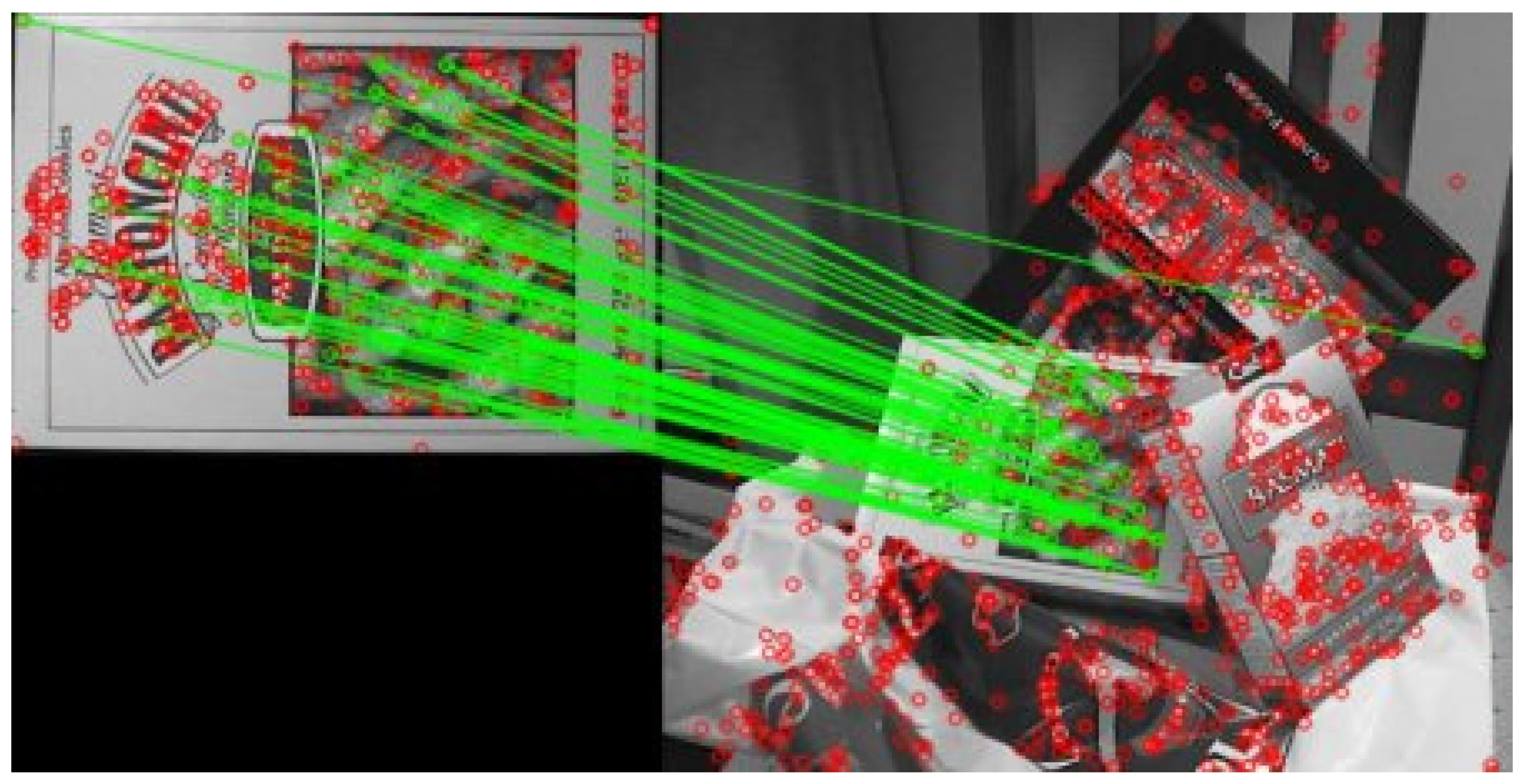
The SIFT algorithm is responsible for the detection of features through computer vision. Each used image undergoes a scan for the detection of recognizable features existing in the image, and these features are stored in a database and compared with the stored features of each new image based on the Euclidean distance of its vectors [39]. Based on this distance and from each matching feature, subsets of points are created (Figure 3). According to the software used, these points are named key points or tie points.

After determining the points (key points or tie points), the BA comes into operation. This algorithm is responsible for refining the coordinates that describe the geometry of the image through the correspondence between the projections of all points. BA is usually the last phase of the first step of a three-dimensional reconstruction, producing a sparse point cloud, formed by the points detected by the SIFT algorithm [40].

After the creation of the sparse point cloud, the next processing step uses the Multi-View Stereo (MVS) algorithms in the sequence of the three-dimensional reconstruction. The MVS algorithms are capable of building highly detailed three-dimensional models from images. Its operation consists of using a large set of images and, from these images, building a plausible three-dimensional geometry that is possible and compatible with some reasonable assumptions, the most important being the rigidity of the scene [42].

For a better understanding, inverting the problem, a photograph can be considered as a three-dimensional projection on a two-dimensional plane, and during this process, the depth information is lost. Starting from an image, it is impossible to reconstruct this lost depth, but with the use of two or more images, through a triangulation process, it becomes possible through the intersection of the projection rays to reconstruct a depth map (Figure 4) [42].

Each of the generated depth maps is combined and filtered to generate a dense point cloud. The next processing step refers to the application of colors to the points, which are obtained from the individual information of the pixels of the photographs used in the three-dimensional reconstruction.

The last step of the three-dimensional reconstruction is the generation of a mesh from the dense point cloud, generated in the previous step by the MVS. This mesh, generated by triangulation of the dense point cloud, can be decimated, as its quality, normally defined by the user at the time of its generation, can vary from low, with minimum values, to very high with the maximum number of faces available. Complementing the mesh, a texture map is generated, adding the RGB information from the pixels of the images that generated the 3D model, to provide a “photorealistic appearance” to the reconstructed object.

The three-dimensional reconstruction of environments and objects may appear simple due to all the facilities of equipment (cameras and UAV) and software for processing the data but invariably holds some surprises.

Unfortunately, most users when starting their processes will come across some survey or some sample that, for some reason, did not present a reconstruction consistent with reality. The most common situations are failures in the reconstruction in the form of holes or large irregularities in surfaces that should be flat, or even large blocks of images that, due to some problem in the algorithms, are in a completely wrong position from where they should be.

The basic algorithms used by the SfM technique have some dependencies for their correct function. The SIFT algorithm, responsible for detecting the features in the images, works correctly when the environment or the sample to be reconstructed presents a certain degree of heterogeneity. It needs elements that are different enough to be detected as a feature and, in the sequence, allows the realization of your correspondence in the neighboring photographs. In some circumstances, the SIFT algorithm can detect features and their correspondences in adverse conditions. These situations would be practically impossible for human eyes to identify.

However, the algorithm is not always able to solve such problems alone, requiring the assistance of the user to solve them. This situation is evident when analyzing Figure 5, where two common types of failures in three-dimensional reconstruction are present. The first type displays a band on the side of the sample where the MVS algorithm was unable to correctly populate the dense point cloud. In the other image, the initial part of the reconstruction pipeline did not adequately reproduce the texture of the sample, which, like the first image, was a cylindrical-shaped sample and should have a regular surface.

Specifically, when working with geological samples, rocks that are homogeneous, such as carbonate rocks, and mainly in the form of a plug will present a significantly higher degree of difficulty for the reconstruction than samples of sedimentary rocks, with an irregular shape and heterogeneity.

2.2. Proposed Methodology

The methodology presented in the article is mainly oriented as a specific application for the three-dimensional reconstruction of geological samples. These samples can be outcrop samples or core samples. Unlike the regular and more general use of these techniques and methodologies, the specificity of the topic forces the adoption of an alternative approach to achieve a model with adequate quality for use in virtual environments.

The proposed methodology aims to provide the user with a continuous and simplified workflow, where each step has its functionality maximized to provide the best possible result. The proposed methodology aims to reduce or even avoid several issues and errors that might occur during the different phases of the three-dimensional reconstruction.

In Figure 6, the workflow describes the main steps of the three-dimensional reconstruction of the samples as well as the methodological elements proposed to optimize the processes.

2.2.1. Procedures for Photo Collection

To ensure the best available image quality, the user must select the appropriate equipment to obtain the photographs, knowing their technical characteristics as well, namely: real focal length and the number and dimensions of pixels in the X and Y axes of the camera sensor. At the present date of this article, the cameras can be separated and selected between two basic types.

The first type is DSLR cameras (Digital Single Lens Reflex), which fit between professional and semi-professional level use and usually have features such as interchangeable lenses and a larger sensor when compared to small cameras (point-and-shoot type). These cameras, due to their interchangeable lenses, allow the use of lenses with a fixed focal length, which reduces or avoids the effect of scale (zoom) in the images. Likewise, the larger sensor allows for more light to be captured, theoretically allowing the collection of an image with greater clarity and vivid details.

The second type would be the cameras present in mid-range to high-end cell phones. These devices, specifically the ones with significantly larger dimensions sensors, when compared to other cell phones, can have resolutions ranging from 48 to 64 megapixels. The images generated by these sensors, despite their reduced dimensions, when compared to photographic cameras, present sufficient sharpness and detail clarity for their use.

The next element that requires attention is the use of a well-illuminated location with diffuse light sources, avoiding the presence of shadows or excessive light sources as much as possible. This type of lighting gives a more natural, realistic and homogeneous appearance to the sample.

From the selection of the camera to be used and the knowledge of its general specifications, using the classic photogrammetric formulas, we can develop the following reasoning to determine the number of images necessary for the three-dimensional reconstruction of an object. This application can be considered ground photogrammetry at a short distance from the object. We can use the equation E = h/f to determine the resolution of each pixel in the image, where E is the scale of the image; h is the flight height; and f is the camera focal length [43]. The scale is a unitless element, so h and f must be used in the same measure unit (e.g., centimeters). In this situation, the flight height element is replaced by the distance between the camera and the object to be imaged. Using a distance of 50 cm between the camera and the sample, on average, can be considered adequate for most regular-size samples. This distance may vary to accommodate smaller or larger samples.

Using a Sony Nex-7 camera as a reference for this article, it has 24 megapixels (MP) of resolution (6000 × 4000 pixels) in its APS-C sensor (23.5 × 15.6 mm) and a 16 mm focal length lens. Applying the values to the equation, we have a 1:31.25 scale for the photographs. Multiplying the scale value by the camera sensor size results in the coverage of each image (footprint) in the X and Y axes, 73.4 cm and 48.8 cm, respectively. Dividing the footprint by the respective number of pixels in the axis, the result is 0.12 mm resolution per pixel, enough to identify very fine sand grains, ranging from 0.0625 to 0.125 mm, according to Wentworth (1922) [44].

The SfM requires a large overlap between the photographs, usually 60% or more due to the need for each reconstructed point must appear and be identified in at least 3 different photographs. To ensure the correct process, it is safer to use at least 75% overlap. In this situation, an object that appears in the first quarter of a photograph will appear at least three more times in subsequent photographs.

To determine an adequate number of photographs for the three-dimensional reconstruction, a circle around the sample based on the 50-cm radius was used as a reference. In this situation, the calculus resulted in a circular perimeter of 3.141 m. As the coverage on the X-axis of the photos is 73.4 cm and with an overlap of 75%, the distance between each of the photos of 18.3 cm totals 17.1 photos for covering the entire perimeter. Rounding up this value to 18, the result is a 20° angle between the photographs, as demonstrated in Figure 7a.

These 18 images refer to the horizontal distribution of the images. In the vertical distribution, the use of a support device to add a space between the sample and the surface is recommended. This separation assists in the reconstruction of the lower edges of the sample. It is recommended to take a set of 18 photographs aligned with the support device, close to 0° from the base of the sample. It is even acceptable for this angle to be a little less than zero, slightly below the base of the sample.

This procedure must be performed again with an angle of approximately 45° from the first set of photos and, to complete the sample coverage, between 3 and 5 photographs at an angle equal to or approximately 90° (Figure 7b). When adding up all the photos in all the positions, the average number of images obtained is 40, but this number may vary slightly depending on the sample size.

These 40 images refer to approximately 83% of the sample, as the face-down side of the sample will be invariably occluded. Therefore, the sample must be rotated on the support, and a new set of images must be obtained. In this situation, usually, the first sequence of images (0° angle) can be discarded since the 45° position presents adequate coverage of the now available occluded face.

At the end of the collection of images, it is essential to check them individually, to ensure that all of them are perfectly in focus and that no anomalies have occurred, such as corrupted files or even white balance problems that might render the images useless.

A practical way to start this check is to visualize the size in megabytes that each image occupies. Given the controlled conditions of the collection performed, the images will show only small differences in the storage space occupied. If any file has a significant difference compared to the others, it means that it must be out of focus. This procedure does not eliminate individual visual analysis but serves to expedite the process.

2.2.2. Aid Elements for Scale and Feature Detection

When a survey is carried out with UAVs, all the obtained images have, at the time of their collection, the register of their spatial position (latitude, longitude and altitude). This three-dimensional information is used during data processing as the initial positioning of each image, allowing the data to be very close to the real scale and with an absolute position better than 4 m in most cases [45]. However, the collection of images of geological samples usually occurs without the possibility of applying any type of active positioning. The only relevant part is determining the correct actual size of the sample.

In this situation, the user must intervene directly in the process and, at the same time, assist in the detection of features. One of the most practical ways for this purpose is the installation of checkered patterns below the samples, with regular or irregular shapes, to aid in feature detection (Figure 8).

The use of these patterns allows a relatively simple way to obtain measurements between points of the checkered patterns and to use this information to perform a sample scaling process, bringing the patterns to the virtual environment in their correct dimensions as in the real world.

As previously mentioned, vertical separation between the object’s base and its support location allows a more detailed reconstruction of the object’s edges, and when it presents problems for positioning, such as keeping the sample vertical, it is recommended to use modeling clay to stabilize the sample. It is also recommended that the color of the support device and the modeling clay be as different as possible from the original color of the sample, which will facilitate the procedure of editing and removing it from the reconstructed model without affecting the quality of the product (Figure 9).

Despite the best practices and efforts, the errors presented in Figure 5 are a reminder that highly homogeneous rocks with regular shapes increase the degree of difficulty for detecting features and correspondence between them in different photographs. In addition to the elements already mentioned, it is possible, in extreme situations, to use small physical markers directly on the samples, which can allow three-dimensional reconstruction. These markers could be small, colored adhesives placed in strategic locations in the sample avoiding the covering of any relevant area.

Another available technique can also be used as a complement to the techniques described so far. In this technique, an arbitrary coordinate system is created, having its origin in the sample. Based on this coordinate system, the user collects the photographs in specific positions and with the camera at a specific orientation. The specific orientation is the camera’s orientation angles at the time of image collection, namely Roll, Pitch and Yaw (Figure 10).

The user can choose if the origin coordinate will be zero or can add a constant value, avoiding the use of negative coordinates. Following the previous example, (a 50-cm radius around the sample) was added to a constant of 5 m on the X and Y axes and 1 m on the Z axis.

For the collection of the photographs for use in this coordinate system, the first step is to collect the 0° elevation photo set, keeping a distance of 50 cm from the sample. The second step is to collect the 45° vertical elevation, but in this position, the horizontal and vertical distance must be reduced to 35 cm, maintaining an inclined distance of 50 cm to the sample. Finally, in the top images, the distance from the sample is maintained at 50 cm vertically (Figure 11).

In addition to the X, Y and Z coordinates of each image, now the dataset has the camera orientation angles and complementary information for every one of the images for use during the processing phase. The inclusion of these angles aims to increase the rigidity of the three-dimensional model reconstruction and also provides scale to the reconstructed model.

The roll and pitch angles are constant, both values being 0° for the first set of photographs and 0° and 45° for the second set. The main variation occurs in the yaw angle, which is equivalent to the azimuth at which the image was collected (

Table 1. Coordinates from the arbitrated system.

Coordinates			Orientation Angle			Coordinates			Orientation Angle
X	Y	Z	Roll	Pitch	Yaw	X	Y	Z	Roll	Pitch	Yaw
5.087	5.492	1.000	0	0	190	5.061	5.345	1.350	0	45	190
5.250	5.433	1.000	0	0	210	5.175	5.303	1.350	0	45	210
5.383	5.321	1.000	0	0	230	5.268	5.225	1.350	0	45	230
5.470	5.171	1.000	0	0	250	5.329	5.120	1.350	0	45	250
5.500	5.000	1.000	0	0	270	5.350	5.000	1.350	0	45	270
5.470	4.829	1.000	0	0	290	5.329	4.880	1.350	0	45	290
5.383	4.679	1.000	0	0	310	5.268	4.775	1.350	0	45	310
5.250	4.567	1.000	0	0	330	5.175	4.697	1.350	0	45	330
5.087	4.508	1.000	0	0	350	5.061	4.655	1.350	0	45	350
4.913	4.508	1.000	0	0	10	4.939	4.655	1.350	0	45	10
4.750	4.567	1.000	0	0	30	4.825	4.697	1.350	0	45	30
4.617	4.679	1.000	0	0	50	4.732	4.775	1.350	0	45	50
4.530	4.829	1.000	0	0	70	4.671	4.880	1.350	0	45	70
4.500	5.000	1.000	0	0	90	4.650	5.000	1.350	0	45	90
4.530	5.171	1.000	0	0	110	4.671	5.120	1.350	0	45	110
4.617	5.321	1.000	0	0	130	4.732	5.225	1.350	0	45	130
4.750	5.433	1.000	0	0	150	4.825	5.303	1.350	0	45	150
4.913	5.492	1.000	0	0	170	4.939	5.345	1.350	0	45	170

).

The user must make the maximum effort to obtain the images at the positions and angles informed, as the dimensional quality of the reconstructed sample depends directly on how accurate the initial position of the collection is. It is worth noting that the processing software itself allows the insertion of uncertainty values for each element and both spatial position and orientation angles; it will recalculate these angles and positions throughout the reconstruction.

2.2.3. Mesh, Solid and Texture Creation

The solid creation presents a great challenge to be performed. Most users simply input all the images obtained in the photograph collection step and hope that the software will be able to perfectly reconstruct the sample. In the majority of cases, this is not the final result. When processing the images through the SfM pipeline, the elements surrounding the sample, which under normal conditions assist the feature detection to stitch the images, in this case, make the process more complex. This occurs due to the difference in the position of the sample on the elevation support in the collection of the two image sets.

In situations where the software can perform the reconstruction properly, the user earns the tedious and delicate task of cleaning the point cloud, removing the remains of the support that will appear in two different places. This task, in addition to demanding a huge amount of time and attention in its execution, can cause problems due to the accidental removal of segments of the sample that may go unnoticed by the user.

To avoid this problem, it is extremely useful and agile to use markers to merge the image sets. The marker placement process is relatively simple, the user just needs to analyze the images obtained from the sample and perform a visual identification of homologous points existing in the two sets (Figure 12).

Each marker has a number that must be placed in the same position in the two sets to perform the correct alignment of the faces. Usually, the set with the highest number of images is defined as the main set and the other as the secondary set. The main set must already be properly scaled to perform this step.

When performing the sets’ merging operation, the user selects the main set as fixed, that is, it will not undergo any type of adjustment. The secondary set will suffer all the adjustments, being scaled, rotated and translated to the same coordinate system as the main set.

After merging the sets, as in the previous steps, an inspection must be carried out to verify the quality of the fit and, if it is adequate, the point cloud cleaning step is carried out. Through this workflow, the dense point cloud cleaning should occur more efficiently because the points that must be removed are at a safe distance from the sample, avoiding the possibility of erroneous removal of sample points. With the point cloud duly edited, the next steps are the point triangulation and the creation of the mesh.

This stage consists of two segments. The first one aims at the construction of the mesh itself and does not present any major complications. The user defines the level of detail that the mesh will have based on the number of polygons that will be obtained in the triangulation. Usually, the average configuration (medium) is used for the mesh. This selection ensures that the model is not oversimplified, losing some relevant geometric feature, or excessively complex, adding a higher computational cost to its use.

With the mesh finalized, the next step is the generation of the photorealistic texture. This texture is responsible for ensuring that the virtual model is an identical digital twin to its real-world counterpart. The texture generation process involves the insertion of some information by the user. Among the information is the image file format that the texture will be generated in, how many textures will be created and what dimension each texture will have.

At first glance, this is too much information for the user, who finds himself without the necessary feedback to generate a texture suitable for its purpose. The most common procedure is to use values much higher than necessary, eventually making it impossible to use the generated model.

For an adequate definition of the dimension and necessary size of the textures, it is recommended to export the mesh in Object File Format (.OBJ) and import it into an external software to measure the dimensions of the mesh information. There are several software programs capable of performing the surface area calculation of the mesh, including some that are free of charge, such as Blender (www.blender.org, accessed on 10 August 2022) [46]. This information is essential because it allows us to calculate the exact number of pixels necessary for the total coverage of the sample without removing any details or adding excessive non-existent information that only increases the size of the model.

As an example, in a model with a surface area of 1000 cm² (100,000 mm²), if we use the area of our spatial resolution of 0.0144 mm² per pixel, obtained from the reference values (0.12 mm per pixel), we will obtain a rounded-up value of 6,944,444 pixels required for the texture. Texture sizes are referenced based on the number of pixels on the X and Y axes. A texture with FullHD dimensions, also known as 1 K, has 1920 × 1080 pixels, that is, 2,073,600 pixels. The texture that comes closest to the value obtained is 4K, where we have 3840 × 2160 pixels, totaling 8,294,400 pixels [47]. Therefore, a texture with 4K dimensions meets the need without adding computational cost for excessive data management. It is also recommended to generate the texture in PNG format. This image file format has a higher visual quality than the JPEG format, which helps its use in virtual three-dimensional visualization systems.

2.3. Methodology Validation Test

To verify the effectiveness of the proposed methodology, a controlled experiment was defined where geology-related personnel performed the three-dimensional reconstruction of geological samples.

Four volunteers were selected, namely:

• An undergraduate student in Geology at the end of the course;
• A Geologist, Master’s student in Geology;
• A Geologist, Ph.D. student in Geosciences;
• A Geologist, Geology Professor.

After the selection of the volunteers, it was defined that each participant would receive the methodological guidelines in an inverse proportional form based on their academic and professional experience. In this experiment, the undergraduate student in Geology received the full complete methodology. The geologist master’s student did not receive information regarding the checkered pattern for scale and how to scale the object. The geologist doctoral student did not receive information regarding the checkered pattern for scale, how to scale the object nor the vertical positions for collecting images. Finally, the geology professor did not receive any information on how to proceed with the three-dimensional reconstruction of the sample (

Table 2. Methodological contents received by the volunteers.

	Undergraduate Student	M.Sc. Student	Ph.D. Student	Geology Professor
Photo Collection Procedures	Complete	Complete	Partial	None
Aid Elements for Scale and Feature Detection	Complete	Partial	None	None
Mesh, Solid, and Texture Creation	Complete	Complete	None	None

).

The data was processed using the Agisoft Metashape software in version 1.7.2 trial (www.agisoft.com, accessed on 10 August 2022) [48]. This choice was made due to the excellent quality of reconstruction obtained in previous activities when comparing the results with other software available on the market.

The methodological information regarding the software operation (except markers), choice of the photographic camera and the environment with diffused lighting were considered relevant but not indispensable or impeditive to the development and execution of the experiment, so these elements were applied in the same way to all volunteers.

For this experiment, a Sony NEX-7 DSLR camera with a resolution of 24 megapixels and a 16-mm fixed focal length lens was used. Three samples were used to validate the methodological process, with each sample presenting a different difficulty level for the three-dimensional reconstruction (Figure 13). The evaluation of the difficulty level of each of the samples had, as an initial reference, the homogeneity of the rock or its constituent minerals, followed by its shape and dimensions.

The initial sample used, identified as Sample 1 (S1), is a carbonate breccia bearing clasts of laminated limestone (laminite) and ferruginous material filling dissolution voids. The sample has dimensions approximately equal to 15 × 15 × 6 cm, presenting a good heterogeneity and an irregular shape, which makes the three-dimensional reconstruction process simpler. This sample was specifically chosen as the most accessible to verify, if under normal conditions; without the necessary methodological knowledge, a sample with a lower difficulty level for the three-dimensional reconstruction process would be adequately reconstructed by the volunteers.

The second sample, identified as Sample 2 (S2), is a bioclastic grainstone with cross stratification and has dimensions approximately equal to 10 × 10 × 8 cm, presenting a higher degree of homogeneity, which adds a degree of difficulty for the three-dimensional reconstruction. This additional difficulty is reduced due to the highly irregular shape of the sample, balancing the process to an easier path.

The third sample, identified as Sample 3 (S3), is a medium to coarse-grained quartzous sandstone with planar cross-stratification and has a half-cylindrical shape of approximately 17 cm with a diameter of 6 cm, presenting a mixed difficulty level due to two main characteristics. The first characteristic that adds difficulty to the process is the shape of the sample. Regular geometric shapes, especially cylindrical ones, significantly reduce the ability of the SfM pipeline to detect features. Its half-core form, that is, half of a standard core cylinder, adds some difficulty to the reconstruction process. The second relevant characteristic of this sample is its constitution. This sample is formed by different minerals with slightly different colors, increasing the heterogeneity of the sample, and therefore reducing the complexity of reconstruction. When comparing all the samples, S1 can be considered the less complex for reconstruction. The S2 and S3 samples present a similar complexity level.

After the completion of the three-dimensional reconstruction process by each of the volunteers, the three-dimensional reconstructions were analyzed quantitatively and qualitatively, considering the following elements:

• Number of images obtained;
• Number of images used in processing;
• Number of points in the point cloud;
• Number of polygons in the mesh;
• Spatial distribution of the images obtained;
• Dimensions of the generated model;
• Geometry of the generated model.

In addition to the analysis carried out, an initial questionnaire was applied so that the volunteers could express their opinions about the activities developed. The questions aimed to identify the difficulties encountered by the volunteers in carrying out the activities as well as their perceptions of the experiment are described below:

• In your opinion, did your three-dimensional reconstruction achieve an acceptable result?
• After the comparison with the reference model, do you think that your reconstruction is acceptable?
• Regarding the steps taken, did you have any difficulties?
• In your opinion, which of the steps presented the biggest challenge?
• In your opinion, were the methodological procedures provided easy to perform?
• In the event of a new three-dimensional reconstruction, would you use the provided methodology?

After completing the first stage of reconstruction and answering the questionnaire, the complete methodology was presented to the volunteers who had not received it fully, and a second stage of reconstruction with a new questionnaire was applied. This questionnaire was based on the Technology Acceptance Model (TAM) methodology [49,50,51], which is based on users’ perceived usefulness and perceived ease of use, indicating how likely the adoption of the technology in question is. For each question, the volunteer selected an answer that varied from likely to unlikely in small increments.

In the 12 presented questions, numbers 1 to 6 determine the user perceived usefulness, and 7 to 12 determine the user perceived ease of use, as follows:

• Using this methodology in my job would enable me to accomplish my tasks more quickly.
• Using this methodology would improve my job performance.
• Using this methodology in my job would increase my productivity.
• Using this product would enhance my effectiveness on the job.
• Using this product would make it easier to do my job.
• I would find this methodology useful in my job.
• Learning to use this methodology would be easy for me.
• I would find it easy to get this methodology to do what I want it to do.
• My interaction with this methodology would be clear and understandable.
• I would find this methodology would be clear and understandable.
• It would be easy for me to become skillful at using this methodology.
• I would find this methodology easy to use.

The perceived usefulness (PU) indicates the subjective probability that a user using a new system or technology will increase his job performance. The perceived ease of use (PEOU) indicates the expected level of effortlessness with which a system or technology can be learned by a user [51]. It is worth noting that, despite the small number of volunteers who participated in the experiment, only four, we believe that, due to the specificity of the activity and the academic heterogeneity, the results obtained will serve as a reference for larger and broader research.

3. Results and Discussion

The models generated by the volunteers were compared, and the models generated by the undergraduate student were set as a reference for comparison, as he received the complete methodological procedure steps. The models were generated in Agisoft Metashape software with the same options throughout the reconstruction process, including the same level of detail for the dense point cloud and the mesh.

The following quantitative elements were compared: the number of photos obtained, the number of photos used in the process, the number of points in the dense point cloud and the number of polygons in the mesh. In addition to the quantitative analysis, we also generated a qualitative analysis of these elements: spatial distribution of photos, model dimensions and model geometry.

Based on the data presented in

Table 3. Results of the first reconstruction previous to the complete methodological procedures.

	Undergraduate Student			M.Sc. Student			Ph.D. Student			Geology Professor
	S1	S2	S3	S1	S2	S3	S1	S2	S3	S1	S2	S3
Number of Photos	59	58	59	59	60	60	43	45	44	32	35	34
Photos Processed	59	58	59	59	60	60	43	45	44	30	34	34
Points on Point Cloud	1.182.369	281.481	958.288	1.173.737	280.126	956.412	985.234	247.464	845.593	838.716	203.510	701.466
Polygons on Mesh	236.472	60.000	191.656	235.265	59.586	189.547	195.045	51.060	158.307	183.787	43.680	140.483

, the difficulties encountered by the volunteers who received partial or no information about the methodological procedures compared to the undergraduate student who was properly trained with the complete methodology become evident.

When analyzing the individual values of each volunteer against the reference values obtained by the undergraduate student, the differences are relevant (

Table 4. Quantitative analysis previous to the complete methodological procedures.

	Undergraduate Student			M.Sc. Student			Ph.D. Student			Geology Professor
	S1	S2	S3	S1	S2	S3	S1	S2	S3	S1	S2	S3
Number of Photos	100%	100%	100%	100%	103.4%	101.7%	72.9%	77.6%	74.6%	54.2%	60.3%	57.6%
Processed Photos	100%	100%	100%	100%	100%	100%	100%	100%	100%	93.8%	97.1%	100%
Points on Dense Cloud	100%	100%	100%	99.3%	99.5%	99.8%	83.3%	87.9%	88.2%	70.9%	72.3%	73.2%
Mesh Polygons	100%	100%	100%	99.5%	99.3%	98.9%	82.5%	85.1%	82.6%	77.7%	72.8%	73.3%

). The first analysis point is the number of photographs collected in each sample. The undergraduate and the master’s student received the complete methodology and performed almost identically in all three samples. The master’s student even collected more photographs in S2 and S3, but extra images do not necessarily mean better results.

The number of photos obtained by the doctoral student on S1 is 27.1% lower than the reference, and the geology professor had a reduction of 45.8%. This behavior, as expected, repeats itself in S2 and S3. Considering the average values from all the samples (S1 to S3), we have a reduction of 25% and 42.6%, respectively.

One of the most important parameters obtained during a three-dimensional reconstruction is the percentage of the images used during the process. If some of the images are not used in the process, we risk obtaining an inadequate model that can present reconstruction failures (holes) or even geometric anomalies in its shape. Comparing the number of processed photos, the geology professor had a 6.3% reduction in the number of images used in the process (30 of 32). This isolated information does not seem to have a great impact, but if we consider that it had a 45.8% reduction in the number of images obtained, this value becomes significant.

Likewise, the number of points in the dense cloud of the doctoral student and the geology professor decreased by 16.7% and 29.1%, respectively, in S1. This scenario does not get much better in S2 with 12.1% and 27.7%, and 11.9% and 26.8% in S3. This point reduction can cause a density reduction in relevant locations, which can distort the sample geometry in a way that may not be identified.

Also, since the dense point cloud is the source for the mesh, a reduction like this significantly reduces the number of polygons generated. The three-dimensional mesh generated by the doctoral and the geology professor showed a reduction of 17.5% and 22.3% in the number of polygons created in the final object in S1. Again, the values of S2 and S3 follow the same trend.

It is not possible to say just by looking at the numbers the quality of the final model obtained, but it is likely that, when comparing the reference model with the model that obtained the lowest values in all categories, the chances of finding defects or not so well recreated areas in the reconstruction will be significantly higher.

The reduced number of photos obtained by the doctoral student (approx. 25% less) and the geology professor (almost 50% less), can be considered a small problem, easily corrected with more practice. This type of conclusion can be reached with more experience performing three-dimensional reconstructions.

All the other elements are directly based on this metric, meaning if we have fewer photos, we will have a reduction in the homologous points detected between the images, reducing the sparse cloud. Fewer pictures also mean fewer points in the dense point cloud and, therefore, fewer triangulations and fewer polygons present in the mesh.

After the initial quantitative analysis, we moved on to the qualitative analysis, where we considered the spatial distribution of the collected images, the dimensions of the model and the geometry of the reconstructed solid. In all the mentioned categories, problems were found, such as the low spatial distribution of the photos, the lack of scale in the model and the incomplete geometry of the solid (

Table 5. Qualitative analysis previous to the methodological procedures.

	Undergraduate Student			M.Sc. Student			Ph.D. Student			Geology Professor
	S1	S2	S3	S1	S2	S3	S1	S2	S3	S1	S2	S3
Spatial Distribution	Good	Good	Good	Good	Good	Good	Medium	Medium	Medium	Low	Low	Low
Model Dimensions	Scaled	Scaled	Scaled	Not Scaled	Not Scaled	Not Scaled	Not Scaled	Not Scaled	Not Scaled	Not Scaled	Not Scaled	Not Scaled
Model Geometry	Solid	Solid	Solid	Solid	Solid	Solid	Open	Open	Open	Open	Open	Open

).

The first qualitative element analyzed was the spatial distribution of the images used for the three-dimensional reconstruction. The spatial distribution of images directly affects the occurrence of irregular density areas along the reconstructed model. In places with a greater number of images, there may be a greater presence of homologous points and, consequently, a greater number of points in the sparse and dense clouds. Likewise, a smaller number of images will reduce the number of homologous points detected as well as a smaller number of points in the sparse and dense clouds.

The undergraduate student and the master’s student received complete methodological information on how to perform the procedure. The doctoral student and the geology professor did not receive the methodological information. Both volunteers who received the methodological information performed the procedure properly, obtaining images with optimized equidistance and positioning for three-dimensional reconstruction. The volunteers who did not receive the methodological information obtained data with reduced quality when compared to the reference element.

In both cases, the images were unevenly distributed, being less noticeable in the case of the doctoral student and more prominent with the geology professor. This irregular distribution may be the main element that caused a failure of unused photos in the geology professor’s three-dimensional reconstruction, additionally causing a significant reduction in sparse and dense point clouds.

The dimensions of the model, that is, its scale, as previously specified, are directly guided by the use of external aids for its correct definition. During or after the first processing step, the user needs to inform some dimension or coordinate that allows the software to assign the real dimensions to the reconstructed model.

The undergraduate student was the only one to use the checkered pattern, which has a dual purpose, the first being to add elements with the possibility of homologous feature detection between the images and, second, to allow the insertion of measurements to scale the model. This procedure is carried out by measuring the checkered pattern and inserting these measurements during processing.

The model geometry was the last qualitative element evaluated. Through this geometry, it is possible to verify if there was any serious failure in the three-dimensional reconstruction and if the user was able to create a closed solid element of the sample. This element is even more relevant during the collection phase where it is necessary to rotate the sample to obtain two sets of images.

When analyzing the reconstructed models, it was possible to verify that only the undergraduate student, who received the complete methodological elements, was able to effectively generate a closed solid. The rest of the volunteers were unable to perform the procedure, resulting in two separate meshes. After the completion of the first reconstruction round and the analysis of the generated data, the volunteers were asked to complete the first questionnaire (

Table 6. Initial perception of the volunteers about 3D reconstruction.

	Undergraduate Student	M.Sc. Student	Ph.D. Student	Geology Professor
In your opinion, your three-dimensional reconstruction achieved an acceptable result?	Yes	Yes	Yes	Yes
After the comparison with the reference model, do you think that your reconstruction is acceptable?	N/A	Yes	No	No
Regarding the steps taken, did you have any difficulties?	No	Yes	Yes	Yes
In your opinion, which of the steps presented the biggest challenge?	Solid Creation	Solid Creation	Solid Creation	Solid Creation
In your opinion, were the methodological procedures provided easy to perform?	Yes	Yes	Yes	N/A
In the event of a new three-dimensional reconstruction, would you use the provided methodology?	Yes	Yes	Yes	N/A

).

When analyzing the answers given to the questions made after the three-dimensional reconstruction of the samples, it is possible to deduce that the perception of model quality and procedures did not reflect the new standards presented to them so far. In the first question, all the volunteers had an opinion that their model was adequate for use, but when compared with the reference model, the doctoral student and the geology professor changed their minds.

In the opinion of all volunteers, the most challenging part was how to create the solid geometry efficiently. Considering that the rock samples can be considered approximately as cubes, it is necessary to rotate the sample to collect photos of the occluded face. In doing so, the surrounding elements are duplicated, namely the table, and everything needs to be manually removed from the dense point cloud before creating the solid mesh, a process that requires considerable attention and time to complete. Using sample elevation support and markers significantly reduces time, making it easier to merge the image sets and ensuring an adequate solid build.

The volunteers that received any methodological orientation stated that the procedures were easy to perform and in an event of a new three-dimensional reconstruction, they would continue to use the procedures.

To put this to the test, in the second stage of the experiment we provide the complete methodological procedures to all volunteers that did not receive the full set earlier and asked them to rebuild the samples. Since the undergraduate student already received the complete methodology, there was no need for him to do the process all over again, but his data was kept as a reference.

The results of the second reconstruction, after all the volunteers received the complete methodological steps are presented in

Table 7. Results of the second reconstruction after the methodological procedures.

	Undergraduate Student			M.Sc. Student			Ph.D. Student			Geology Professor
	S1	S2	S3	S1	S2	S3	S1	S2	S3	S1	S2	S3
Number of Photos	59	58	59	59	60	60	60	59	59	61	60	61
Photos Processed	59	58	59	59	60	60	60	59	59	61	60	61
Points on Point Cloud	1.182.369	281.481	958.288	1.180.348	282.335	957.863	1.183.114	281.998	958.379	1.184.557	282.441	959.012
Polygons on Mesh	236.472	60.000	191.656	235.978	60.127	192.513	236.114	60.051	191.284	237.002	61.015	192.574

. The qualitative analysis of the numbers shows a regularity between the newly reconstructed models and the reference (

Table 8. Quantitative analysis after the methodological procedures.

	Undergraduate Student			M.Sc. Student			Ph.D. Student			Geology Professor
	S1	S2	S3	S1	S2	S3	S1	S2	S3	S1	S2	S3
Number of Photos	100%	100%	100%	100%	103.4%	101.7%	101.7%	101.7%	100%	103.4%	103.4%	103.4%
Processed Photos	100%	100%	100%	100%	100%	100%	100%	100%	100%	100%	100%	100%
Points on Dense Cloud	100%	100%	100%	99.8%	100.3%	99.9%	100.1%	100.1%	100%	100.2%	100.3%	100%
Mesh Polygons	100%	100%	100%	99.8%	100.2%	100.4%	99.8%	100.1%	99.8%	100.2%	101.7%	100.5%

).

Comparing the results from the first reconstruction with the results from the second reconstruction, the numbers increased significantly. All the obtained results are grouped in a small percentual margin of −0.2% to +3.4%. These variations are expected since each volunteer collected their images in a similar way but in slightly different positions from each other.

A very important element that showed an excellent result was the number of photos used in the process. All the images taken by the volunteers were used during the reconstruction, a different scenario when compared with the first reconstruction where the geology professor had some images not used.

The improvement can also be identified in the qualitative analysis (

Table 9. Qualitative analysis after the methodological procedures.

	Undergraduate Student			M.Sc. Student			Ph.D. Student			Geology Professor
	S1	S2	S3	S1	S2	S3	S1	S2	S3	S1	S2	S3
Spatial Distribution	Good	Good	Good	Good	Good	Good	Good	Good	Good	Good	Good	Good
Model Dimensions	Scaled	Scaled	Scaled	Scaled	Scaled	Scaled	Scaled	Scaled	Scaled	Scaled	Scaled	Scaled
Model Geometry	Solid	Solid	Solid	Solid	Solid	Solid	Solid	Solid	Solid	Solid	Solid	Solid

), where all the analyzed elements were fulfilled by the volunteers. The images had a good spatial distribution, with the correct angle and distance between each other in all sets. All the models were in the correct size, confirming that the applied scale worked. And the last, but the most visually relevant of the elements is the model geometry. In the first reconstruction, only the undergraduate and the master’s received the procedure to merge the image sets using markers and were able to execute the task. All volunteers were able to create the solid, enabling its use on any virtual applications or the Geological Samples Database.

In Figure 14 we have the three reconstructed models in the same virtual environment, ready for use. There are several software for the visualization of 3D models, but only a few have specific tools that allow for extracting relevant information. One free software that has this capability is CloudCompare v2.12.4 [52], freely available at www.cloudcompare.org (accessed on 10 August 2022). The software CloudCompare v2.12.4 can open several formats of objects and point clouds, making it ideal for this type of data.

After the completion of the reconstructions and the analysis, we reach the final step of the experiment, the TAM questionnaire (

Table 10. Technology Acceptance Model Perceived Usefulness.

Perceived Usefulness	Likely						Unlikely
	Extremely	Quite	Slightly	Neither	Slightly	Quite	Extremely
1. Using this methodology in my job would enable me to accomplish my tasks more quickly.	3	1
2. Using this methodology would improve my job performance.	3	1
3. Using this methodology in my job would increase my productivity.	3	1
4. Using this product would enhance my effectiveness on the job.	4
5. Using this product would make it easier to do my job.	4
6. I would find this methodology useful in my job.	4

and

Table 11. Technology Acceptance Model Perceived Ease-of-Use.

Perceived Ease-of-Use	Likely						Unlikely
	Extremely	Quite	Slightly	Neither	Slightly	Quite	Extremely
7. Learning to use this methodology would be easy for me.	2	2
8. I would find it easy to get this methodology to do what I want it to do.	3	1
9. My interaction with this methodology would be clear and understandable.	3	1
10. I would find this methodology would be clear and understandable.	4
11. It would be easy for me to become skillful at using this methodology.	4
12. I would find this methodology easy to use.	3	1

). The 12 questions are designed to provide a better understanding of this methodology and to identify if it has the capabilities of being assimilated by the users on their daily basis work. As stated previously in this work, the reduced number of volunteers does not allow tendency-free statistic results. Therefore, the given answers were adapted to a normalized scale, with the extremely unlikely attributed value of 0 and the extremely likely value of 6.

As demonstrated by the answers given by the volunteers, the feedback provided was significantly positive. Of 48 answers received from the volunteers, 40 (83.3%) were extremely likely and 8 (16.7%) were quite likely. The individual answers for each question resulted in normalized values ranging from 0.92 to 1.00, providing an average value of 0.98 for the perceived usefulness and 0.97 for the perceived ease of use. These results corroborate the quantitative and qualitative analyses previously executed in both reconstruction series.

4. Conclusions

This article presented a unified methodological proposal for the three-dimensional reconstruction of geological samples aiming for its use in virtual applications or a Digital Samples Database environment. This methodological proposal was structured to improve the workflow in the three-dimensional reconstruction of geological samples, which relies directly on elements such as the heterogeneity, dimensions and overall shape of the samples to produce usable results with adequate visuals and geometric quality.

Despite being a procedure that has been used for some years and may present high-quality results, the use of three-dimensional reconstruction for geological samples is a field that has not been extensively explored yet, given the large number of recent articles that use this technique to create DOM. These models are usually produced for insertion in immersive virtual reality environments, a recent trend in recent years, especially since the arrival on the market of devices such as the HTC Vive and the Oculus Rift.

These two devices opened a new chapter for consumer use of virtual reality. Previously, immersive visualization systems were limited to systems such as Cave Automatic Virtual Environment (CAVE) or L-Shape, notoriously expensive with complex and restricted use. Both devices are portable and can be used in medium to high-end computers with compatible graphics cards.

The main contribution of this paper is providing a unified methodological workflow for the three-dimensional reconstruction of geological samples. This research focuses on facilitating user access to a unique methodology that preemptively analyzes and solves the main problems and some exceptional ones that may occur during the three-dimensional reconstruction of geological samples. This article has delved deeper into the methodologies for collecting photographs, in addition to the implementations to assist the SIFT algorithm and edge reconstruction.

The present research highlights the need to use a solid methodology for the three-dimensional reconstruction of rock samples, especially for operators with little to no knowledge of the subject. Most papers treat three-dimensional reconstructions as a by-product, spending no more than a small paragraph in the text on this subject.

As a small methodological test, it served to validate the workflow, as well as to measure the perception of the volunteers regarding the methodology itself, its strengths and weaknesses. This objective is well-defined by the use of three samples with different characteristics ranging from a sample that can be considered simple to reconstruct, very heterogeneous and with an average size that allowed its easy manipulation by the volunteers, to more difficult and complex samples.

This is usually the normal situation when approaching the analysis of siliciclastic rocks or any other igneous or metamorphic rock that presents heterogeneous visuals and irregular shape. However, especially when working with carbonate rocks, their homogeneity grows significantly, making it difficult for the software to find the analog characteristics necessary for proper processing. This difficulty can be increased by the shape of the sample. The regular geometric shapes present a greater challenge for three-dimensional reconstruction, mainly the cylinder. The reduced number of edges and irregular surfaces mine the SfM algorithm’s capability to identify features.

In the continuity of this research, the focus will be on increasing the number of volunteers to address a more adequate TAM statistics. This approach, despite being the most technically adequate, presents considerable logistical challenges, as the activities will have to be carried out using the same camera and the same samples to produce overall valid results.