Horizontal-to-Vertical Spectral Ratios and Refraction Microtremor Analyses for Seismic Site Effects and Soil Classification in the City of David, Western Panama

Abstract

The City of David constitutes one of the most important commercial centers of the Republic of Panama. However, it is located on a coastal plane, close to an area with high seismic activity and has been affected by significant earthquakes (18 July 1934, Mw = 7.4 and 12 March 1962, Mw = 6.7). The goal of this study is to estimate the seismic effects and to classify the soil in the City of David. The experimental work entailed the measurement of environmental noise for H/V spectral ratio (HVSR) analyzed at 22 stations. A series of microtremor refraction studies (ReMi) at six stations distributed from north to south of the city was also performed. The stations were distributed around urban areas of the city, which are characterized by the presence of water supply, sewerage, buildings, roads, etc. The spectral analysis of environmental noise allowed the generation of three different types of maps: First, predominant frequency maps (f₀) with zones composed mainly of rigid and semi-rigid soils in the southern end of the city and rigid soils in the central and northern regions. Secondly, maximum H/V amplitude maps (A₀) which evidence a low range of HVSR amplitude in the city, ranging from 1.1 to 3.8. Finally, liquefaction vulnerability (K_g) maps, with values less than 2 Hz⁻¹, representative of a low liquefaction risk. Soil classification using ReMi and calculation of the corresponding V_s30 reveal type D soils, which correlate well with results obtained using HVSR analyses. A comparison between HVSR and ReMi shows that HVSR curves that exhibit clear peaks tend to be related to ReMi stations that presented relatively large shear-wave velocity contrasts at some depth. The results from this research are intended to aid the decision-making process related to the future development of the city, as well as government level maintenance and mitigation plans.

1. Introduction

Natural disasters such as earthquakes, floods and storms can generate emergencies related to shortages of drinking water and damage to buildings and road networks in a given city. In order to ensure the safety and functionality of the structures of human settlements, it is necessary to have a broad knowledge of the physical and geotechnical characteristics of the soils. In some cases, this can be solved by the development of geotechnical studies.

The analysis of seismic effects at sites close to urban areas of high seismicity by using geotechnical tests, requires definition with a significant density of sampling points. In many cases, the areas where studies must be carried out are well urbanized. Thus, it becomes difficult to develop traditional geotechnical testing. As a result, this generates a high investment of both time and money, because these types of tests are subject to unforeseen events or circumstances that could arise during the development of such activities, not to mention the expenses related to equipment mobilization. In addition, most of the available data are proprietary.

The challenges of implementing traditional geotechnical testing can be solved by using geophysical methods, such as the analysis of the spectral ratio H/V of microtremors or HVSR. It is a robust method that seeks to estimate the predominant frequencies of a soil profile through an analysis of environmental noise records.

Although [1,2] first applied this technique, Ref. [3] popularized it. Ref. [3] demonstrated the similarities between the spectral ratio of the horizontal and vertical components of a microtremor record, and the transfer function of the surface layers for horizontal movement. The method also offers information on the levels of local amplification and risk of liquefaction of the soils.

Some authors have applied this method to assess the impact that seismic amplification has had on civil structures affected by past earthquakes [4,5], for the evaluation of the liquefaction potential of soils [6,7], for studies of amplification of areas for future civil projects [7,8], for the assessment of the impact of earthquakes on existing civil structures typical of urban environments [9,10,11], in studies related to landslides [12,13], in coastal and port areas [4,9,14,15] and for the site characterization of seismic stations [16,17,18]. In Panama, several studies have been carried out on the estimation of side effects in some cities [19,20,21].

The City of David is considered one of the most important places of the Isthmus of Panama. It is the main commercial center of the region and also an important logistic hub. The most common economic activities are related to agriculture and livestock, allowing the development of important industrial manufacturing and the communications sector.

The City of David has hospitals, schools, undergraduate educational centers and universities, shopping centers, hotels and it is an important tourist spot. However, it is characterized by presenting frequent seismic activity due to its proximity to the Panama Fracture System, in which the Panama sub-plate and the Cocos and Nazca tectonic plates converge.

The research presented in this paper represent a fraction of the grant SENACYT IOMA19-11 (entitled: Seismic Vulnerability of Water Supply Networks in Panama), which aimed to develop a seismic vulnerability framework in zones of the city supplied by water pipelines and a method to take into account soil properties (predominant frequency, amplification, etc.). As a result, most of the measurement stations (HVSR and ReMi) are located within the city center which lays predominantly in one geological formation. Thus, the planning and design of the measurement campaign must be analyzed taking into account this fact, because not all geological formations will be covered. By funding such research projects, the national government intends to generate databases of different parameters, which are non-existent right now.

The objective of this work focuses on assessing horizontal-to-vertical (H/V) spectral ratio of microtremors in the City of David, western sector of the Isthmus of Panama. This is achieved through a series of measurements of the seismic site effects and by mapping the predominant frequency of subsoil, the corresponding maximum amplitude of the spectral ratio H/V and the liquefaction vulnerability index K_g. In addition, refraction microtremor (ReMi) geophysical tests are conducted to estimate 1-D shear wave velocity profiles and the average shear wave velocity (V_s30). These tests are carried out throughout the city by using multichannel analysis of surface waves in order to verify the former results and classify the soils of the city.

2. Area of Study

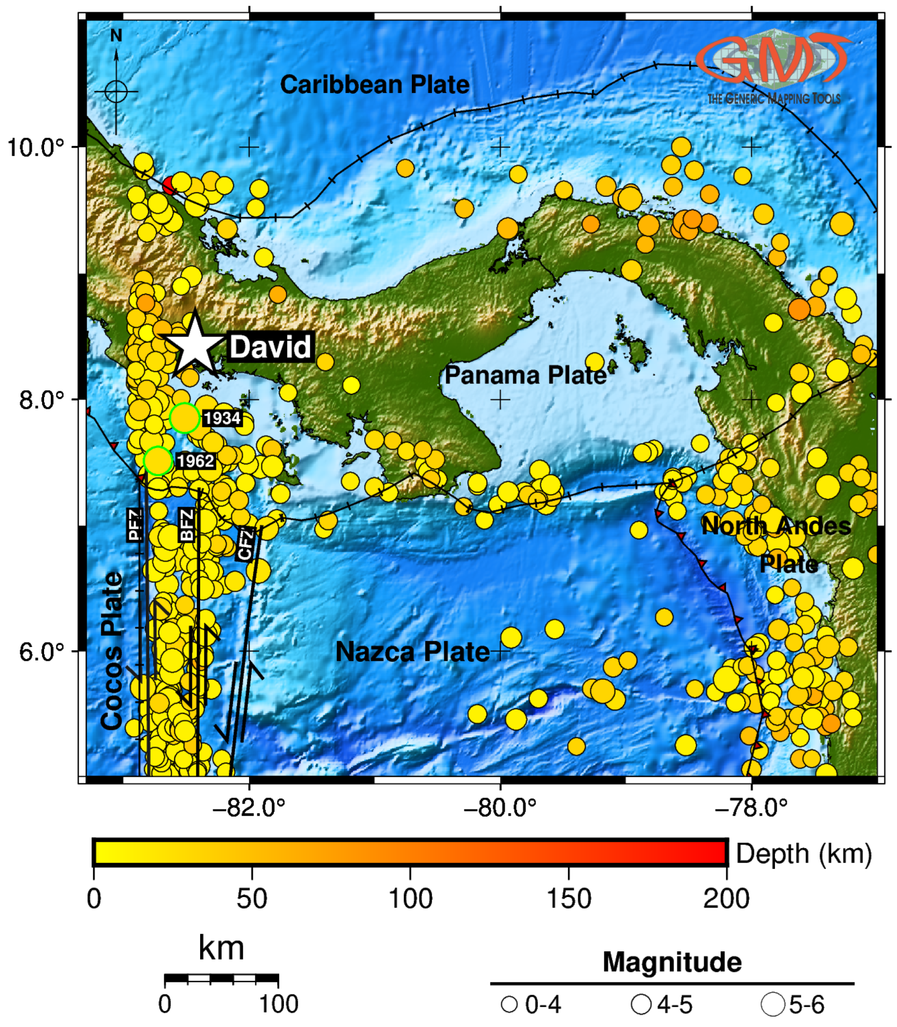
2.1. Seismicity and Tectonics of the City of David and Surrounding Areas

The Panama Fracture System extends from the Costa Rican ridge, between the coordinates 3° and 6° north latitude and between 83° and 82° west longitude. At around 6° in a northerly direction, this system is made up of a set of faults running parallel and in a dextral direction. The zones of greater seismicity in the isthmus, the Panama Fracture Zone (PFZ), the Balboa Facture Zone (BFZ) and the Coiba Fracture Zone (CFZ) [22] are located in this area (Figure 1).

PFZ constitutes the western boundary of the Panama Fracture System, which is the limit between the Nazca and Cocos plates. The PFZ originated approximately 1 million years ago at the same time as the subduction of the Cocos ridge (Figure 1). The tectonic activity of this area still prevails.

BFZ is located in the center of the Panama Fracture System. According to [23] it has a high seismicity. The highly reflective ridge in this zone is slightly asymmetrical, with a steep section on the west side towards the Panama Fracture Zone.

Finally, CFZ is in the eastern part of the Panama Fracture System. Its mountain range is defined by a wide zone in a northerly direction. The eastern side of the Coiba mountain range presents directions between 2° and 7° to the northeast [22].

Seismic activity in Panama is relatively moderate in comparison with its neighboring countries: Costa Rica and Colombia. The country’s historical seismicity has been studied by several authors. Most of these available studies have been focused on addressing the seismicity of the areas surrounding the Panama Canal, both from measuring stations, instrumental seismicity, as well as from paleoseismic studies for assessment of historical seismicity. Two noteworthy historical seismic events are the earthquakes of 1621 (5.6–7.0 Mw) and of 1882 (Mw 7.9–8.0) [24,25].

The western region of the Isthmus of Panama is characterized by presenting a significant number of seismic events. One of the most damaging events has been the 1991 earthquake of Limon–Changuinola (Mw = 7.7, Depth = 10 km, Epicenter: Limon, Costa Rica), which produced severe damage to the province of Bocas del Toro, located in the north of the province of Chiriqui. This earthquake (IX MMI) was felt from Tegucigalpa through Panama City. This event resulted in more than a thousand casualties (79 deaths and 1061 wounded). Moreover, more than 1060 structures were reported with structural collapse [26].

In the case of the City of David (located in the province of Chiriqui), there is an important amount of seismic activity in comparison to other cities of the country. Between the years 2015 through 2022, an approximate of 13,475 earthquakes of different magnitudes have been reported. Of those, 5238 events originated in the province of Chiriqui. This number represents roughly 39% of the reported earthquakes [27].

Two of the most noteworthy seismic events in David are the earthquakes of 18 July 1934, Mw = 7.4 and 12 March 1962, Mw = 6.7. Macroseismic data is very scarce in Panama, particularly for earthquakes that happened such a long time ago. The earthquake of 18 July 1934 is known as “The Puerto Armuelles Earthquake”. It had a magnitude of Mw = 7.4 and a focal depth of 25 km. The epicenter was located in the Gulf of Chiriqui. Reported intensity scales range from IX MMI in Puerto Armuelles (50 km from David) through V MMI in Panama City (350 km from the epicenter) and V MMI in San Jose, Costa Rica (300 km from the epicenter). The event and its aftershocks produced extensive damage on the southwest coast of Panama, especially in areas where alluvial materials are known to exist. The cost of the damage is estimated at USD 1.7 million in 1932 [28,29,30].

This large magnitude event was felt from Panama through Costa Rica. In the Gulf of Chiriqui, the earthquake created a crack along Montuosa Island about 60 to 90 cm wide and 6 m deep, passing near triangulation towers. The shock was violent in Parida Island. It caused two or three landslides that forced the few inhabitants to abandon the island. At Puerto Armuelles, the shock was felt very strongly and was of long duration, causing several blackouts. Fans were reported to be swinging and in some cases striking the ceiling. Historical reports indicate that only a few houses were destroyed and no well-built structures in the town suffered serious damage. In contrast, the water pipes and sewage in the city, and the oil pipeline and pumping stations at the docks were broken. In the City of David, the shock caused panic, walls crumbled, some adobe houses collapsed and roofs caved in, injuring a number of people [31].

The earthquake of 12 March 1962 occurred near the south coast of Panama and Costa Rica. Historical information reports show that some damage was caused to the City of David and surrounding areas. No available data were found on this earthquake’s intensity. The shock was felt in the Valle del General at San Vito and Helechales and was reported from San Jose (Costa Rica). The earthquake was rather strong at Balboa Heights, Panama City. A vessel sailing 33 km off Punta Burica reported feeling the earthquake. Moreover, it has been associated with small tsunamis recorded at Puerto Armuelles and Galapago Islands. This main earthquake was followed by a number of aftershocks that caused more damage in the City of David [31].

Figure 1. Geographic location of the City of David on the relief map obtained through pyGMT and the seismicity of the Isthmus of Panama including Panama Fracture Zone (PFZ), Balboa Fracture Zone (BFZ) and Coiba Fracture Zone (CFZ) [32,33].

Figure 1. Geographic location of the City of David on the relief map obtained through pyGMT and the seismicity of the Isthmus of Panama including Panama Fracture Zone (PFZ), Balboa Fracture Zone (BFZ) and Coiba Fracture Zone (CFZ) [32,33].

2.2. Geological Context

The geology of the Isthmus of Panama has been studied to some extent [34]. Initially, it was inferred from marine geology studies [33,35,36,37,38] which were complemented with geology studies from the border zone with Costa Rica [39]. The geology of inland areas has been partially addressed [40] in some cases motivated by the oil and gas industry [39]. However, despite these studies, geological information in Panama tends to be scarce. There is only a national map which presents a generalized distribution of geological formations. There are no regional geology maps. In addition, this map presents limited information. Only superficial formations are shown, and there are no available geologic profiles in the country.

The City of David is located in the southwestern sector of the Isthmus of Panama (Figure 2a). It rests on a vast plain made up of clays, laterites and alluvium (Figure 2b). There is a relatively thick stratum of soft soil in the south and center of the city. There are rocky outcrops (i.e., volcanic) in the northern side, as well as in an area located in the extreme south. These outcrops manifest themselves as hills made of intrusive volcanic rock [19].

Four geological formations can be identified in the study area. First, the Baru Quaternary formation, which is linked to successive eruptions of the volcano of the same name and is characterized by the volcanic context of the region. This formation spreads laterally around the volcano´s edifice. This formation typically consists of a sandy soil matrix with few fines. The soil is relatively well graded. Soil particle shape tends to be angular (close to the volcano) to rounded (sites far from the volcano).

Second, the Las Lajas Quaternary formation is the result of an accumulation of sedimentary deposits in a deltaic context. The deposits are of various natures but all of them come from fluvial transport, together with the existence of a mangrove swamp near the ocean with warm and shallow areas, which explains the presence of coral remains.

The Senosri–Uscari tertiary formation suggests a continental soil deposit characterized by the presence of calcareous tuff material. These elements are the result of the precipitation of dissolved carbonate ions in water in the continental context (lake, stream, pond, etc.). Finally, the Tonosí tertiary formation is characterized by a shallow marine-type deposit, which explains the presence of both sandstone and shales.

3. Research Methodology

Earthquake site effects and seismic site classification were assessed using two environmental vibration analysis methods. The first one is related to the analysis of horizontal-to-vertical (H/V) spectral ratios from microtremors, by using tri-axial devices and selecting a local transfer function. The second one implies using a linear array of low frequency seismic sensors (1-component) to obtain a dispersion curve extracted from surface waves phase velocity spectra. Inversion processes are carried out to obtain the velocity distribution for shear waves (or S-waves) with respect to depth.

3.1. Microtremor’s Horizontal-to-Vertical Spectral Ratio

This technique utilizes either microtremor records or environmental noise obtained from a tri-axial station to estimate the predominant frequency of sedimentary layers which typically lay over rock substratum. The study uses the concepts introduced by [3] for the study of microtremor spectral ratios.

The transfer function (S_TT) proposed by [3] can be expressed as the quotient between the spectral ratio of the horizontal components measured at the surface and the rock stratum (S_T = H_S/H_R) and the spectral ratio of the vertical components measured at the surface and rock substratum (E_S = Λ_S/Λ_R). Assuming that the quotient of the horizontal and vertical component of the rock substratum is equal to one, then the transfer function for surface layers can be estimated by using microtremors measured at the surface, essentially: S_TT = S_T/E_S = Hs/Λ_S.

The result of this type of analysis is usually presented as a peak value in a semi-logarithmic graph of the spectral ratio H/V as a function of frequency. This peak value is associated with both the predominant frequency of the soil (f₀) as well as the maximum value of the spectral ratio H/V (also known as A₀). The value of A₀ is considered to be the HVSR amplitude of the superficial layers, caused by the multiple reflections of the horizontal shear waves at the frequency f₀ [42].

According to [43], environmental noise time-series records represent the convolution of source effects, source-to-receiver propagation effects, instrumental effects and site response. These effects are multiplied in the frequency domain, under certain assumptions. A division operation between the Fourier amplitude spectra of the horizontal and vertical components allows elimination of the first three effects, leaving only the site response effects.

For risk quantification of future structures prior to the occurrence of seismic events, adopted international standards suggest classifying the type of site. Some of the standards worth mentioning are those presented by [44,45].

Table 1. Definition of site classification for this project according to [44,45].

Site/Class	Natural Period (s)	Predominant Frequency (Hz)
SC I: rock/stiff soil	TG < 0.2	f0 > 5
SC II: rigid soil	0.2 ≤ TG < 0.4	2.5 < f0 ≤ 5
SC III: semi-rigid soil	0.4 ≤ TG < 0.6	1.6 < f0 ≤ 2.5
SC IV: soft soil	TG ≥ 0.6	f0 ≤ 1.6

presents these specifications, taking into account the period and the predominant frequencies of the soil. This criterion has been previously implemented in Panama by [21], where the criterion presented in Table 1 is combined together with that of NEHRP [46], which is commonly used for site-specific ground response analyses in the civil engineering industry. The resulting criterion uses predominant frequency (or natural period) as a means to infer an expected soil class and correlate that with NEHRP classification.

3.2. Liquefaction Vulnerability Index for Subsoil

Another important parameter that can be estimated from f₀ and A₀ is the liquefaction (or subsoil) vulnerability index (K_g). Although this parameter can be interpreted as a risk assessment factor, it can also be used as a proxy to infer whether the soil is prone to liquefaction phenomena when subject to the action of a seismic event [47]. This value is derived from the stresses that the subsoil experiences and is defined as K_g = A₀²/f₀ by [48].

The liquefaction vulnerability index is closely related to the loss of shear stress in the soil which also depends on the soil deformation. Therefore, it can be an indicator of liquefaction: the higher the values of K_g, the higher the possibility of liquefaction. Several studies have shown the occurrence of liquefaction phenomena for K_g values greater than 10 [6,48,49].

3.3. Refraction Microtremor Method (ReMi) and Classification Using V_s30

ReMi method is a passive seismic geophysical method proposed by [50] where environmental noise characteristic of urban environments (passage of vehicles, machinery in operation and other active sources) is analyzed as a microtremor. The ReMi method analyzes surface waves (Rayleigh and Love) to determine the distribution of shear wave transmission velocity (V_s) through the ground to a depth that depends on the maximum wavelength of the surface wave.

The result is a one-dimensional shear wave velocity profile. Applications for ReMi range from soil characterization to land surveying and assessment for civil works. In a similar way as other surface-wave based methods, ReMi takes advantage of the dispersive nature of such waves. In other words, at different frequencies the wave train travels at different speeds. When considering a stratified soil, the high-frequency components are influenced by the superficial layers while the low-frequency ones are influenced by the deeper strata [51].

As the Rayleigh-type surface wave is coupled to the vertical component of the shear wave, the V_s distribution in a stratified terrain generates a velocity spectrum that combines a frequency with the Rayleigh wave phase velocity. Upon interpretation of the spectrum, a dispersion curve can be obtained. This spectrum is indicative of the energy associated with the Rayleigh wave which describes an envelope of a high spectral rate that goes from low to high frequencies.

Since the ReMi method can generate one-dimensional profiles of V_s, it is therefore possible to measure the average value of the shear wave velocity down to a depth of 30 m (V_s30) in order to characterize a site. It should be noted that the method is not reliable by itself. The results need to be compared to additional independent data (either from other non-surface geophysical tests or from geotechnical testing) and the resolution of the data with depth affects all surface methods. The reliability of the method can be improved by using additional constraints like HVSR curve during inversion. In this study, the joint inversion approach has not been implemented.

According to [52,53,54], the value of V_s30 represents a robust parameter that has been adopted for the characterization of the site response. Previous research [10] points out the usefulness of this parameter in building codes, earthquake-resistant designs and seismic zoning studies in urban environments.

Table 2. Type of soil profile classification according to the NEHRP [46] based on the average shear rate to a depth of 30 m.

Soil Type	General Description	Vs30 (m/s)
A	Hard rock	Vs30 > 1500
B	Rock	760 < Vs30 ≤ 1500
C	Hard and/or very stiff soil	360 < Vs30 ≤ 760
D	Rigid soils	180 < Vs30 ≤ 360
E	Semi-rigid soils	Vs30 < 180
F	Soils that require specific calculations	Does not apply

shows the classification of soils according to NEHRP [46].

These criteria (Table 2) will be used together with that presented in Table 1. The criterion presented in Table 1 allows classification of soil based on fundamental frequencies, whereas the one in Table 2 requires the usage of the average shear wave velocity in the upper 30 m of soil.

3.4. Limitations of HVSR and ReMi Methods

In current practice, both HVSR and ReMi methods have been widely accepted, since both methods are low-cost alternatives to obtain a general idea of the site characterization. However, there are advantages and limitations to both ReMi and HVSR methods [14,43,55].

For all types of passive geophysical methods (such as ReMi), the dispersion curve that is obtained undergoes a series of issues. First and foremost, the fundamental mode is not necessarily the dominating one and the continuity of a signal does not imply that a single mode is involved. There are directionality issues: the technique relies on a linear array of geophones, whereas seismic events from unknown sources could be perpendicular to the array direction. In addition, some of the possible pitfalls of implementing the ReMi technique could be related to the experiment itself. The length of the geophone array must be consistent with the depth of the bedrock.

Towards this end, errors such as selecting lines that are too short, miscalculating geophone spacing, recording for too little time could have an important impact on the test itself [51,56,57]. For this reason, it is very common to develop some type of geotechnical testing together with these types of geophysical tests. However, doing so, undermines the advantage typical of a non-destructive test. In the particular case of this study, no geotechnical information has been included. Thus, this fact needs to be accounted for when using the data of this study for future projects or endeavors.

HVSR has been used for site characterization. However, a likely issue with this method is the fact that the amplification from actual earthquakes will be noticeably different than HVSR predictions [58]. Towards this end, [58] also indicates that HSVR measurements cannot be assumed as a direct estimate of the amplification function, because it deviates significantly from it. Indeed, site effects from an earthquake will be determined by the properties and features of its source [59]. The readings from ambient noise will very likely differ from those of actual seismic activity.

Despite the aforementioned issue, in many cases, soils will exhibit low HVSR amplitude factors due to their composition and material properties. Thus, in many previous studies, HVSR data are reported as they were measured [5,6,60,61,62,63,64]. In such cases, caution must be exerted, because these values should not be used for analysis or design of civil infrastructure.

In recent years, the professional community tends to treat and analyze these methods as if they were geotechnical tests, which they are not. Both ReMi and HVSR remain as some of the techniques that allow some level of site soil characterization without the need of sophisticated test or expensive equipment. The purpose of the data and methodology presented herein is to aid, with scientific evidence, the decision-making process for government agencies and population in general. This situation is particularly common in developing countries, where seismic stations are scarce and research resources are limited. In those cases, the use of such techniques can provide insightful information for decision- and policy-maker personnel. It is not adequate for design purposes.

4. Data Acquisition and Processing Strategy

4.1. HVSR

Twenty-four (24) stations distributed in the City of David in areas with little traffic were selected (see Figure 2). However, the results obtained in two of these stations presented drawbacks due to certain environmental restrictions such as anthropic factors that occurred in the vicinity.

The equipment used in this study was a portable tri-axial seismograph of the GEOtiny type (from GEObit) with dynamic range and an RMS of 129 dB. The device has a sampling frequency of 100 Hz and a GPS antenna that allows a specific time to be associated with the records obtained in the field. Recording duration was set to 28 min. UTM geographic coordinates were considered and measured using a portable GPS. During measurement time, the seismograph was covered with a plastic box to avoid the recording of unwanted noise produced by the wind.

Each one of the environmental vibration records were processed with the software Geopsy, which is a tool developed by the European project SESAME (2004) [65]. Files in miniSEED format were exported in such a way that they can be separated and viewed for each component. A band-based filter was applied in order to attenuate those signals below 0.05 Hz and above 20.0 Hz, and a Tukey-type window of 5% width was used.

The filtered signal was divided into windows of specific duration (25.0 s for this study) in order to eliminate the abrupt maximums (noise) due to anthropic effects. At this stage, it was necessary to select only sections of the signal where its amplitude is almost stationary. For this purpose, an STA/LTA anti-trigger algorithm was applied and its quotient corresponded to the amplitude of the record in a short-time window (STA = 1.0 s) and a long-time window (LTA = 30.0 s). Next, a rectangular window filter of constant width and frequency of 1.0 Hz was applied for smoothing. Finally, an output frequency range between 0.5 and 20.0 Hz was established in such a way that the software (Geopsy) could generate an H/V spectral ratio curve.

The next step consisted of verifying whether the maximums obtained in each of the stations correspond to a stratigraphic type effect (which provides the value of the predominant frequency of the subsoil f₀), or to an anthropic or industrial type effect, which is not represented in this type of study.

For this purpose, the values of the spectral-energy density of the three components were plotted jointly as a function of frequency. The three graphs are then examined at the value of fundamental frequency corresponding to the maximum HVSR amplitude. If at said frequency, the values given by the horizontal components (north–south and east–west) are higher than the vertical component, then the maximum HVSR amplitude obtained is assumed to be due to stratigraphic effects and not anthropic or industrial. Due to the typical shape presented by the three curves obtained in the frequency value where the maximum of the H/V spectral curve is reported, this effect is known as an “eye-shaped curve” [6,12,21,62,66].

To visualize the previously mentioned effects, Figure 3 presents a sequence of the analysis for two stations of this study to illustrate the stratigraphic (Figure 3a) and anthropogenic (Figure 3b) type effect. The graphs at the top correspond to the environmental noise records in each component. The graphs placed at the center of these same figure represent the H/V spectral curves and the lower graphs are the energy spectral densities associated with stratigraphic and anthropogenic effects, respectively. The areas in green in the upper graphs (Figure 3a,b) represent the time windows that were selected to carry out the calculation of the H/V spectral ratio.

SESAME [65] project has issued guidelines for assuring the quality of HVSR data. The first step before processing any dataset is to verify whether the set is reliable under a series of criteria which must be fulfilled before further analyses or interpretation can be carried out. These are:

• The fundamental frequency of f₀ must be greater than 10 divided by the window length of l_w, for the peak to be significant;
• The significant cycles number must be greater than 200;
• HVSR curve standard deviation amplitude, at a range frequency of 0.5 f₀ to 2 f₀, must be <2 when f₀ > 0.5 Hz, or < 3 when f₀ < 0.5 Hz.

Additional guidelines are also presented to ensure clear peak selection. These guidelines are widely accepted in the literature [65]. However, many sources have reported that in some cases the selection of clear peaks can become a somewhat challenging task [8,11,17,67,68,69]. Even though in a simple visual inspection of the data, several sites with apparently clear peaks might be noticeable, applying this criterion sometimes fails to identify many of these peaks [67]. This is particularly true for HVSR curves that do not visually exhibit a pronounced peak. Ref. [68] reinforces this notion, indicating that the six SESAME criteria for a clear HVSR peak are well suited for measurements with relatively pronounced peaks. According to [68], for all other cases, such as broad, asymmetrical, multiple peaks, or HVSR near unity or “flat”, an automated selection process may fail, thus measurements should be assessed in a site-by-site basis, requiring experienced judgement.

4.2. Multichannel Analysis of Surface Waves (MASW) and V_s30

Six (6) ReMi seismic surveys were developed in specific areas of the City of David, as shown by the distribution of the boxes in light green in Figure 2. For each seismic survey, 24 low-frequency vertical geophones were used (4.5 Hz) and interconnected to a seismograph (PASI). Geophones were separated with a distance of 2 m between them. This distance was set according to the restrictions and obstacles that the urban landscape of the city presented, such as the presence of modern structures and streets. At each station, 20 files were generated with 24 noise signals of a duration of 32 s, and a sampling interval of 2 ms was chosen.

Each of the 6 sets of 20 files was separately processed by using Eliosoft’s winMASW Professional-2023 software [70]. High frequency refracted waves and other unwanted signals were removed from the seismic traces through of a temporary windowing process. Subsequently, the records in the time domain were transformed to obtain a phase velocity spectrum. Next, a set of data pairs representing the values of phase velocity versus frequency (dispersion curve) was obtained. For this purpose, the spectrum was selected along the lower bound of phase velocity instead of the section where the maximum energy is concentrated.

Finally, the inversion of the dispersion curve was carried out by defining an initial model and a search for the parameter space (space of the shear wave velocity/layer thickness values) according to the dispersion curve. The winMASW Professional-2023 software is based on the use of genetic algorithms to carry out the inversion of the dispersion curve automatically [70].

For the optimization process, 80 generations were established. The best model was chosen to be the one presenting the least mismatch or error. The parameterization of the model was based on the assumption of a one-dimensional model constituted by a set of linearly elastic homogeneous layers and stacked under a half-space. Through this process, it is possible to find a model for the average shear wave velocity and its standard deviation by means of a statistical approximation. The latter can be done based on the estimation of the marginal posterior probability density (MPPD) [70].

5. Results

5.1. Spatial Distribution of H/V Spectral Ratios

Data for (1) predominant frequency of the subsoil, (2) maximum value of the H/V spectral curve associated with the predominant frequencies and (3) values of the liquefaction vulnerability index calculated from the first two, were interpolated and represented as maps, to assess the spatial distribution of these subsurface parameters.

Results obtained in the H/V spectral ratio analysis for each station are presented in

Table 3. Values of the predominant frequency of the soil (f₀), maximum value of the spectral ratio H/V (A₀) and liquefaction vulnerability index (K_g) obtained in each of the 22 stations.

Station	UTM Coordinates (m)	f0 (Hz)	A0	Kg (Hz−1)
E01	341879 → 925069	6.5	1.7	0.4
E02	343069 → 926258	2.7	1.2	0.5
E03	342503 → 927833	4.2	2.1	1.1
E06	343863 → 925982	1.9	1.6	1.3
E07	343334 → 931171	11.0	1.7	0.3
E08	343541 → 926773	9.0	2.0	0.4
E09	341608 → 928320	3.4	1.4	0.6
E10	341903 → 931798	6.9	3.7	2.0
E11	344019 → 933809	11.0	1.3	0.2
E12	341807 → 933456	10.7	1.9	0.3
E13	343628 → 934452	7.0	2.2	0.7
E14	339485 → 929806	9.7	1.9	0.4
E15	342563 → 932566	8.6	2.7	0.8
E16	341238→931334	11.0	3.8	1.3
E17	343834 → 935632	9.9	1.7	0.3
E18	338409 → 931254	14.0	2.6	0.5
E19	342711 → 930259	7.4	2.7	1.0
E21	342349 → 935696	7.6	2.2	0.6
E22	344593 → 936622	13.6	1.1	0.1
E23	341328 → 929227	6.1	1.4	0.3
E24	343199 → 929526	11.0	2.3	0.5
E29	340856 → 930933	6.7	2.2	0.7

. Individual spectra for each station are presented in the Appendix (Figure A1 and Figure A2).

All the recorded data is considered reliable according to the previously mentioned SESAME [65] guidelines (i.e., it complies with the three criteria for reliability) (

Table 4. SESAME criteria for data reliability. For this study, l_w = 25 s.

No.	Criterion	Range	Reliable
1	f0 > 10/lw	[1.9–14.4 Hz] > 0.4 Hz	Ok
2	nc > 200	[2517–17,120] > 200	Ok
3	σA < 2	[0.23–1.31] < 2	Ok

). However, regarding the criterion for clear peaks, many of the recorded data exhibit spectral curve shapes with no visually clear peak. Indeed, these curves tend to be broad or flat. Application of SESAME [65] criteria for clear peak selection results in the identification of clear peaks in 10 of the 22 stations. The remaining 12 stations exhibit both moderate as well as no-clear peaks. In those stations, SESAME criteria [65] is not able to identify clear peaks (phenomenon previously explained in this paper). Thus, the selection of peaks is done using previously mentioned criteria (Section 4.1) and expert judgement.

Figure 4 presents two examples corresponding to the characteristic types of H/V spectral curves identified in this study with their respective energy spectral densities. As mentioned before, 10 out of 22 stations exhibit H/V spectral curves with well-defined maximums (i.e., clear peaks) similar to the Type A spectrum shown in Figure 4. Values for A₀ are found to be greater than two. These are defined as HVSR Type A curves. Fundamental frequencies and HVSR amplitude for these stations range between 4.2 to 14.0 Hz and 2.1 to 3.8, respectively.

The remaining 12 stations are classified as HVSR Type B curves. They exhibit shapes that range from being broad with a somewhat defined maximum, to other curves that tend to be very flat. Frequencies for these spectra and HVSR amplitude range from 1.9 to 13.4 Hz and 1.1 to 2.0, respectively.

From the data obtained, three different maps are generated through Kriging interpolation methods: (1) predominant frequency (f₀), (2) maximum value of the spectral ratio H/V (A₀) associated with said frequencies and (3) liquefaction vulnerability index (K_g). Figure 5a shows the spatial distribution of the predominant frequency (f₀) with a range of values between 1.9 and 14.0 Hz.

The low frequencies (f₀ ≤ 4.2 Hz), represented by purple and light blue tones, are concentrated in a large part of the southern sector of the city, except for the extreme south where the predominant frequency reaches a value of 6.5 Hz. This is a sector close to the mangrove area and is characterized by the presence in part of alluvium, consolidated sediments, other characteristic elements of the Las Lajas formation and by volcanic ash and other elements typical of the Baru formation, both formations from the quaternary period. The intermediate and high frequencies (f₀ > 6.0 Hz) are concentrated in the intermediate and upper zones of the City of David, where a large part of the studied area is influenced by the geological elements of the Baru formation (volcanic rocks, volcanic ash, tuffs, agglomerates and lava).

Figure 5b presents the spatial distribution of A₀. The total range extends from 1.1 to 3.8 and is represented through yellow and green shades. The low values (A₀ < 2.7) represented in yellow are concentrated in a large part of the city while the range of A₀ values between 2.7 and 3.7 (in green) and is identified in the central area of the City of David.

Figure 5c shows the spatial distribution of the liquefaction vulnerability index (K_g) estimated from the f₀ and A₀ values. The values of this parameter range from 0.1 to 2.0 Hz⁻¹, where the low values (K_g < 1.3 Hz⁻¹) represented in brown are concentrated in a large part of the studied area while the higher values (K_g ≥ 1.3 Hz⁻¹), which are represented in light blue, are concentrated in the central part of the city.

5.2. Distribution of V_s30 Values from MASW Studies

The analysis of the ReMi records generated in each of the six stations (R-1 through R-6 of Figure 2) resulted in the phase velocity spectra, as shown in Figure 6.

For each of these spectra, the picked points (phase velocity versus frequency) are displayed in pink, the points in blue correspond to the response of the best model as a product of the 1D inversion and the points in green correspond to the average of the models considered. It is observed that these points tend to be located at similar spots. Thus, the quality of the inversion process for each survey is deemed to be adequate.

The results of this 1D inversion process are displayed in Figure 7. For each station, the best calculated statistical model of the dispersion curve is presented (solid line in blue), with the average model of the dispersion curve (dotted line in red) obtained from all models considered (solid lines in gray) as well as the parameter space (in light green).

Below each 1D model, there is a graph that shows the evolution of the discrepancy during the calculation process for both the average (red dotted line) and best model (solid blue line). As can be seen in these graphs, for a total of 80 generations, the discrepancies obtained in all the probes for the best model tend to be minimized (1.56–7.84).

Table 5. V_s30 values obtained in each ReMi survey and their respective classification according to the NERHP (see Table 2).

Station	UTM Coordinates (m)	Vs30 (m/s)	Soil Classification
R-1	341914 → 925077	259 ± 1	D
R-2	342869 → 928047	369 ± 7	C
R-3	342392 → 930351	300 ± 15	D
R-4	342630 → 931976	335 ± 10	D
R-5	343689 → 933689	360 ± 4	D
R-6	343690 → 935579	319 ± 8	D

presents the results of the 1D inversion for each ReMi survey developed in the area of interest.

By comparing Table 5 with Table 2, it can be concluded that almost all the ReMi surveys carried out can be classified as type D soils (rigid soils), except survey R-2, which presents a type C classification (very dense soil); when considering the dispersion of the average value (±7 m/s), however, it is very close to type D soil.

6. Discussion

6.1. H/V Spectral Ratios

Considering SESAME criteria [65] results obtained in all stations comply with the three first criteria, which are related to the reliability of the H/V curves. However, when considering criteria for clear peaks, 10 out of 22 stations (45%) satisfy the criterion established for the value of A₀ (>2.0). These (Type A) are mainly located in the north and central parts of the City of David (Baru formation), except for stations E03 and E18 which are near the limits of the Baru formation and Las Lajas formation.

The results for the remaining 12 stations (which amount to 55%) did not satisfy the second set of SESAME [65] criteria for clear peak selection (Type B). The map in Figure 8, shows that the majority of these readings were obtained near the limits of the Baru and Las Lajas formations.

Care must be exerted when interpreting the location of each station and its possible correlation to the geology of the city. As it was mentioned in previous sections, geological information in Panama tends to be scarce and limited and the map presented in this paper was obtained from a national map which depicts the geology of the country to some extent.

By visual inspection, it seems to be that most of the Type A spectra fall in the areas corresponding to the Baru formation, while the Type B spectra surrounds the city and tend to be located near the limits of Baru and Las Lajas formations. However, there are cases, such as stations E18 and E03, which are also located in the peripheral area of the city and are Type A. The latter is located, strictly speaking, in Las Lajas formation but exhibits an HVSR amplitude factor very close to two.

Low frequencies (≤4.2 Hz) that are concentrated in a large part of the southern sector of the City of David (Figure 5a) are associated with semi-rigid soils in the extreme southeast and hard soils in the rest of said sector according to [44,45], shown in Table 1.

In the same context, the value of the predominant frequency obtained in the extreme south of the city suggests the existence of a rigid soil. The presence of two geological formations of a sedimentary (Las Lajas) and volcanic (Baru) type in this sector of the city may be associated with the low range of predominant frequencies obtained in this study.

Regarding the predominant intermediate and high frequencies (>6.0 Hz) identified in the intermediate and upper areas of the City of David, all of them are associated with rigid soils in accordance with the aforementioned international standard. This physical characteristic of the soils is largely associated with the presence of the particular geological elements of the Baru volcanic formation.

The range of the maximum values of the spectral ratio H/V (A₀) presented in Figure 5b can be classified as low (≤3.8), which means that the HVSR amplitude levels of the soils of the studied area are not high. The range of values of the liquefaction vulnerability indices (K_g) spatially displayed in Figure 5c can also be classified as low according to various studies carried out. Therefore, the risk that the soils present liquefaction phenomenon under the occurrence of seismic events is significantly low.

6.2. Results for V_s30

The values of the V_s30 obtained from the multichannel analysis of ReMi-type surface waves (MASW) in each of the six stations established in the City of David allow verification of the validity of the spatial distribution of the f₀ values obtained through their interpolation process.

According to the NEHRP [46], almost all stations are classified as soil type D, which corresponds to rigid soils. Additionally, according to the interpolated values of the map in Figure 5a, f₀ > 6.1 Hz at all stations; therefore, they are also associated with rigid soils (SC I) according to [44,45].

However, the R-2 station presents a discrepancy between both international standards because the value of V_s30 exceeds 360 m/s (see Table 4) and therefore, it is classified as type C soil corresponding to a very dense soil. At this same station, the value of the predominant frequency resulting from the interpolation process is 6.1 Hz, which corresponds to rock/stiff soil (SC I). In this same context, if the dispersion presented by the average value of V_s30 obtained at station R-2 is taken into account, the proximity to the type D classification can be verified.

6.3. Comparison of Results from HVSR and ReMi

By using the location of the measurement stations for HVSR and ReMi studies shown in Figure 2, it is possible to develop qualitative comparisons between the ReMi stations (1 through 6) and HVSR stations that share a similar or close location to them. Previous sections mentioned that this study does not encompass geotechnical tests. Moreover, inversion of HVSR curves has not been developed. Instead, the comparison will be made by using the criteria introduced in this paper, which combines both [46] and [44,45], which has already been implemented by [21].

Comparison of stations E17 and R-6 is perfectly plausible, since they are located very close to each other. Both stations fall within the area corresponding to Baru formation, but very close to Tonosi formation. HVSR data for station E17 indicate a fundamental frequency of 9.9 Hz and an HVSR amplitude of 1.6. According to Section 6.1, the HVSR curve obtained at station E17 is of Type B: no clear peak. Using criteria outlined in Table 1, this corresponds to a SC I soil (rock/stiff soil). ReMi studies carried out at station R6 produced a soil classification of Type D, with a V_s30 of 319 m/s. The shear velocity profile (Figure 8) shows the existence of a relatively soft soil layer (176 to 235 m/s) down to a depth of around 10 m, followed by a somewhat stiffer soil (V_s = 440 m/s).

A somewhat valid comparison can be made between HVSR station E13 and ReMi station R-5, which are located relatively close to each other. Station E13 presented a predominant frequency of 7.0 Hz and HVSR amplitude of 2.2. The HVSR curve corresponding to station E13 is of Type A, with a well-defined clear peak. Criteria outlined in Table 1 indicate that this should be a SC I soil (rock/stiff soil). On the other hand, ReMi studies produced a Type D soil classification, with a V_s30 of 360 m/s. The shear wave velocity profile corresponding to this station shows initial soil strata extending to a depth of around 7.3 m, with V_s values ranging between 211 and 231 m/s. These strata overlay a stratum of stiffer soil, which presents V_s values of around 482 m/s.

For a comparison of station R-4, the closest HVSR station is E15. This station presented values of f₀ = 8.6 Hz and A₀ = 2.7 and is classified as SC I: rock/stiff soil. The HVSR curve associated with station E15 is of Type A. On the other hand, R-4 (V_s30 = 335 m/s) exhibits a shear velocity profile consisting of a relatively soft soil with V_s ranging from 170 to 251 m/s, followed by a stiffer stratum with V_s = 419 m/s. Site classification for station R-4 is Type D.

Next, station E19 (f₀ = 7.4, A₀ = 2.7, SC I: rock/stiff soil) can be compared to station R-3 (V_s30 = 300 m/s, soil type D), which has a shear wave velocity profile starting at 292 m/s and followed by two layers of softer soil (V_s = 195 m/s and 209 m/s). This profile then increases abruptly to 470 m/s at a depth of around 14 m below surface. The HVSR curve corresponding to station E19 is of Type A.

A similar phenomenon is observed when comparing station E03 (f₀ = 4.2, A₀ = 2.1, SC II: rigid soil) and station R-2 (V_s30 = 369 m/s, soil type C). The shear wave velocity profile corresponding to the latter presents relatively low velocity values (129 m/s < V_s < 224 m/s) at shallow depths, followed by a large velocity contrast (V_s = 528 m/s) at a depth of 5.2 m. The HVSR curve for station E03 is of Type A.

Finally, the HVSR results obtained at station E01 (f₀ = 6.53, A₀ = 1.7, SC I: rock/stiff soil) can be compared to those from station R-1 (V_s30 = 259 m/s, soil Type D). These stations are geographically located at the same coordinates. Their location also corresponds approximately to the limits of the Baru, the Las Lajas geological formation and the southern part of the city. Similar to station E17, the HVSR curve for station E01 is of Type B, which exhibits no clear peaks according to SESAME [65] criteria.

Two interesting observations arise from this discussion:

• First, stations located at the northern (R-6 and E17) and southern (R-1 and E01) ends of the city present no clear peaks according to SESAME [65] criteria (Type B). These stations happen to be located near the limits of Baru geological formation and other formations (i.e., Tonosi formation in the north and Las Lajas formation in the south). On the other hand, the rest of the stations fall clearly into the area corresponding to Baru formation. All of them exhibit clear peaks and, thus, are of Type A.
• Second, inspection of the shear wave velocity profiles for all the six ReMi stations allows us to infer that stations which presented velocity contrasts of ΔV ≥ 249 m/s at some depth can be associated with HVSR stations that exhibit clear peaks (HVSR curves of the Type A). In contrast, the stations that presented ΔV < 249 m/s are located close to HVSR stations with curves of Type B. This observation is in agreement with that presented by [11]. According to their research, whenever the HVSR peak is clear, then the site under study presents a large velocity contrast at some depth. They supported this fact with Fourier amplitude spectra computed from strong ground motion stations [11].

7. Conclusions

The predominant frequency (f₀), the HVSR amplitude (A₀) and the liquefaction vulnerability index (K_g) are parameters that can be used to estimate site characterization effects. These parameters were measured in 22 stations in the City of David through an HVSR analysis of ambient noise.

The range HVSR amplitude factors obtained in this study, the morphology of the HVSR curves and the well-established SESAME criteria [65] allowed classification of the spectral curve in two types: A and B, as defined in previous sections. The former corresponds to curves that exhibited clear peaks. The latter encompasses spectra for which the definition of peaks is not completely clear according to the aforementioned criteria [65].

Three maps have been produced (Figure 5a–c), which represent the spatial variability of the measured parameters in the City of David. Predominant frequencies present a range of values between 1.9 and 14 Hz. Low frequencies tend to be located towards the southern sector of the city. Intermediate and high frequencies are concentrated in the middle and upper zones of the City of David.

HVSR amplitude is mapped in Figure 5b and ranges from 1.1 to 3.1. Low values of HVSR amplitude have been measured in a large portion of the surveyed area of the city. Intermediate values tend to be located in the central area of the city.

Third, liquefaction vulnerability indices (K_g) are presented in Figure 5c. Values range from 0.1 to 2.0 Hz⁻¹. The distribution of these values is similar to that of the HVSR amplitude. The center of the city presents values of K_g in the upper range (1.9 Hz⁻¹), while the rest of the city presents lower values of K_g. Comparison of these measurements with the interpretation criterion reported by Nakamura [3,47] yields that the likelihood of observing liquefaction phenomena in the City of David is relatively low.

The spatial distribution of the predominant frequencies in the City of David allowed identification of semi-rigid soils and stiff soils in the southern part of the city. Rigid soils were identified in the central and north areas. This finding is consistent with the distribution of the different types of H/V spectral ratios (Type A and Type B, for clear and unclear peaks, respectively) throughout the city. It can be observed that Type A curves tend to be located towards the center and north of the city, where the Baru formation is predominant. A site classification has been performed, which is also consistent with the geology of the area. Said classification was verified and validated by using ReMi tests, together with a classification criterion that combines guidelines from [44,45] and NEHRP [46].

Comparison between results from ReMi stations and those from HVSR stations closely located to one another allows us to infer that clear peaks are associated with the existence of large shear wave velocity (V_s) contrasts at some depth. In the case of this study, the two stations that presented low velocity contrasts were placed both at the northern and southern limits of the city. These stations showed HVSR curves with no clear peaks (Type B). On the other hand, the rest of the stations, which are located towards the central portion of the city, exhibited curves of Type A, with clearly defined peaks. The shear wave velocity profiles of these ReMi stations present relatively large contrasts at certain depths through the profile. A similar observation was discussed by [11].

Although HVSR and ReMi methods are widely accepted in current industry practice, they both have limitations. A likely issue with HVSR is that it relies on ambient noise whereas the site effects from an earthquake are determined by the properties and features of both the underlying soil and the seismic source. Thus, it is important to emphasize the qualitative value of HVSR measurements for estimating amplification, although it can definitely be used to distinguish different soil types and other usages.

As explained in previous sections, this research was part of a broader research project which aimed to develop a seismic vulnerability study in zones of the city supported by water supply infrastructure. As a result, most of the measurement stations are located within the city center (which lays predominantly on Baru formation), which is urbanized and developed.

As a result of this research, a database of seismic parameters has been developed for the City of David. The distribution of parameters A₀ and K_g are indicative of a reduced risk of soil liquefaction in the event of an earthquake in the City of David. Given the lack of available data in the country, the results herein presented (such as the maps for predominant frequency, HVSR amplitude and liquefaction vulnerability index) could be used by local authorities to support decision-making processes prior to the construction of civil works.

References

1. Nogoshi, M.; Igarashi, T. On the Propagation Characteristics of Microtremor. J. Seismol. Soc. Jpn. 1970, 23, 264–280. [Google Scholar]
2. Nogoshi, M.; Igarashi, T. On the Amplitude Characteristics of Microtremor (Part 2). Zisin (J. Seismol. Soc. Jpn. 2nd Ser.) 1971, 24, 26–40. [Google Scholar] [CrossRef]
3. Nakamura, Y. A Method for Dynamic Characteristics Estimation of Subsurface Using Microtremor on the Ground Surface. Q. Rep. Rtri. 1989, 30, 25–33. [Google Scholar]
4. Panou, A.A.; Theodulidis, N.; Hatzidimitriou, P.; Stylianidis, K.; Papazachos, C.B. Ambient Noise Horizontal-to-Vertical Spectral Ratio in Site Effects Estimation and Correlation with Seismic Damage Distribution in Urban Environment: The Case of the City of Thessaloniki (Northern Greece). Soil Dyn. Earthq. Eng. 2005, 25, 261–274. [Google Scholar] [CrossRef]
5. Vergara, L.; Verdugo, R. Características Del Terreno de Fundación de Sitios Con Edificios Dañados Severamente En El Terremoto Del 27F. Obras. Y Proy. 2017, 21, 46–53. [Google Scholar] [CrossRef]
6. Bora, N.; Biswas, R.; Malischewsky, P. Imaging Subsurface Structure of an Urban Area Based on Diffuse-Field Theory Concept Using Seismic Ambient Noise. Pure Appl. Geophys. 2020, 177, 4733–4753. [Google Scholar] [CrossRef]
7. Mohamed, A.; Ali, S.M.; Mostafa, A. Estimation of Seismic Site Effect at the New Tiba City Proposed Extension, Luxor, Egypt. NRIAG J. Astron. Geophys. 2020, 9, 499–511. [Google Scholar] [CrossRef]
8. Talha Qadri, S.M.; Nawaz, B.; Sajjad, S.H.; Sheikh, R.A. Ambient Noise H/V Spectral Ratio in Site Effects Estimation in Fateh Jang Area, Pakistan. Earthq. Sci. 2015, 28, 87–95. [Google Scholar] [CrossRef]
9. Pentaris, F.P. A Novel Horizontal to Vertical Spectral Ratio Approach in a Wired Structural Health Monitoring System. J. Sens. Sens. Syst. 2014, 3, 145–165. [Google Scholar] [CrossRef]
10. Ramírez Gaitán, A.; Flores Estrella, H.; Preciado, A.; Bandy, W.L.; Lazcano, S.; Alcántara Nolasco, L.; Aguirre González, J.; Korn, M. Subsoil Classification and Geotechnical Zonation for Guadalajara City, México: Vs30, Soil Fundamental Periods, 3D Structure and Profiles. Near Surf. Geophys. 2020, 18, 175–188. [Google Scholar] [CrossRef]
11. Bonnefoy-Claudet, S.; Baize, S.; Bonilla, L.F.; Berge-Thierry, C.; Pasten, C.; Campos, J.; Volant, P.; Verdugo, R. Site Effect Evaluation in the Basin of Santiago de Chile Using Ambient Noise Measurements. Geophys. J. Int. 2009, 176, 925–937. [Google Scholar] [CrossRef]
12. Pazzi, V.; Tanteri, L.; Bicocchi, G.; D’Ambrosio, M.; Caselli, A.; Fanti, R. H/V Measurements as an Effective Tool for the Reliable Detection of Landslide Slip Surfaces: Case Studies of Castagnola (La Spezia, Italy) and Roccalbegna (Grosseto, Italy). Phys. Chem. Earth Parts A/B/C 2017, 98, 136–153. [Google Scholar] [CrossRef]
13. Iannucci, R.; Martino, S.; Paciello, A.; D’amico, S.; Galea, P. Engineering Geological Zonation of a Complex Landslide System through Seismic Ambient Noise Measurements at the Selmun Promontory (Malta). Geophys. J. Int. 2018, 213, 1146–1161. [Google Scholar] [CrossRef]
14. Di Stefano, P.; Luzio, D.; Renda, P.; Martorana, R.; Capizzi, P.; D’Alessandro, A.; Messina, N.; Napoli, G.; Todaro, S.; Zarcone, G. Integration of HVSR Measures and Stratigraphic Constraints for Seismic Microzonation Studies: The Case of Oliveri (ME). Nat. Hazards Earth Syst. Sci. Discuss. 2014, 2, 2597–2637. [Google Scholar] [CrossRef]
15. Salazar, W.; Mannette, G.; Reddock, K.; Ash, C. High-Resolution Grid of H/V Spectral Ratios and Spatial Variability on Microtremors at Port of Spain, Trinidad. J. Seism. 2017, 21, 1541–1557. [Google Scholar] [CrossRef]
16. Di Giulio, G.; Cultrera, G.; Cornou, C.; Bard, P.-Y.; Al Tfaily, B. Quality Assessment for Site Characterization at Seismic Stations. Bull. Earthq. Eng. 2021, 19, 4643–4691. [Google Scholar] [CrossRef]
17. Alexopoulos, J.D.; Dilalos, S.; Voulgaris, N.; Gkosios, V.; Giannopoulos, I.K.; Kapetanidis, V.; Kaviris, G. The Contribution of Near-Surface Geophysics for the Site Characterization of Seismological Stations. Appl. Sci. 2023, 13, 4932. [Google Scholar] [CrossRef]
18. Leyton, F.; Leopold, A.; Hurtado, G.; Pastén, C.; Ruiz, S.; Montalva, G.; Saéz, E. Geophysical Characterization of the Chilean Seismological Stations: First Results. Seismol. Res. Lett. 2018, 89, 519–525. [Google Scholar] [CrossRef]
19. Toral, J.; Ho, C.A.; Lindholm, C.; Tapia, A.; Chichaco, E. Amplificación Sísmica de Los Suelos de David Chiriquí, Capítulo V de La Microzonificación Sísmica de David, Report; Instituto de Geociencias up, Ngi, Norsar and Cepredenac: Panama City, Panama, 2000. [Google Scholar]
20. Echeverría Durán, Y. Microzonificación Sísmica de La Ciudad de Puerto Armuelles Mediante La Técnica de Nakamura Provincia de Chiriquí, Panamá; Instituto de Geociencias: Panama City, Panama, 2011. [Google Scholar]
21. Ladrón De Guevara, J.; Mojica, A.; Ruiz, A.; Ho, C.; Rodríguez, K.; Toral, J.; Fabrega, J. Ambient Noise H/V Spectral Ratio in Site Effect Estimation in La Mesa de Macaracas, Panama. Int. J. Geophys. 2022, 2022, 6171529. [Google Scholar] [CrossRef]
22. Tapia, A. Zonificación Sísmica de La Región Occidental de La Provincia de Chiriquí. Bachelor’s Thesis, Universidad de Panama, Panama City, Panama, 1996. [Google Scholar]
23. Adamek, S.; Frohlich, C.; Pennington, W.D. Seismicity of the Caribbean- Nazca Boundary: Constraints on Microplate Tectonics of the Panama Region. J. Geophys. Res. 1988, 93, 2053–2075. [Google Scholar] [CrossRef]
24. Víquez, V.; Camacho, E. El Terremoto de Panamá La Vieja Del 2 de Mayo de 1621: Un Sismo Intraplaca. Boletín De Vulcanol. 1993, 13, 13–20. [Google Scholar]
25. Rockwell, T.; Gath, E.; Gonzalez, T.; Madden, C.; Verdugo, D.; Lippincott, C.; Dawson, T.; Owen, L.A.; Fuchs, M.; Cadena, A.; et al. Neotectonics and Paleoseismology of the Limon and Pedro Miguel Faults in Panama: Earthquake Hazard to the Panama Canal. Bull. Seismol. Soc. Am. 2010, 100, 3097–3129. [Google Scholar] [CrossRef]
26. Montero, W.; Pardo, M.; Ponce, L.; Rojas, W.; Fernández, M. Evento Principal y Replicas Importantes Del Terremoto de Limón. Rev. Geológica América Cent. 1994, Special volume: Terremoto de Limon, 93–102. [Google Scholar]
27. Alexander, H.H.E.; Medrano de González, E.; Almengor, C.; Jorge, L.; Espino, J.A. Inventario de Las Incidencias de Los Desastres En La República de Panamá al 2022; Report; Ministry of Economics and Finance: Panama City, Panama, 2023. [Google Scholar]
28. Arroyo, I. Sismicidad y Neotectónica En La Región de Influencia Del Proyecto Boruca: Hacia Una Mejor Definición Sismogénica Del Sureste de Costa Rica. Bachelor´s Thesis, Universidad de Costa Rica, San José, Costa Rica, 2001. [Google Scholar]
29. Camacho, E. The Puerto Armuelles Earthquake (Southwestern Panama) of July 18, 1934. Rev. Geológica América Cent. 1991, 13, 1–13. [Google Scholar] [CrossRef]
30. Víquez, V.; Toral, J. Sismicidad Histórica Sentida En El Istmo de Panamá. Rev. Geofísica 1987, 27, 135–165. [Google Scholar]
31. Ambraseys, N.N.; Adams, R.D. The Seismicity of Central America; Imperial College Press: London, UK, 2000; ISBN 978-1-86094-244-0. [Google Scholar]
32. Morell, K.D.; Fisher, D.M.; Gardner, T.W. Inner Forearc Response to Subduction of the Panama Fracture Zone, Southern Central America. Earth Planet Sci. Lett. 2008, 265, 82–95. [Google Scholar] [CrossRef]
33. Cowan, H.A.; Sánchez, L.; Camacho, E.; Palacios, J.; Tapia, A.; Irving, D.; Esquivel, D.; Lindholm, C. Seismicity and Tectonics of. Western Panama from New Portable Seismic Array Data; NTNF-NORSAR: Kjeller, Norway, 1996. [Google Scholar]
34. IRHE-BID-OLADE Informe Final Del Estudio de Reconocimiento de Los Recursos Geotermicos de La República de Panamá; Latin American Energy Organization: Quito, Ecuador, 1987.
35. Heil, D.; Silver, E. Forearc Uplift South of Panama. A Result of Transform Ridge Subduction. Geol. Soc. Am. Abstr. Prog. 1987, 19, 698. [Google Scholar]
36. McKay, M.; Moore, G.F. Variation in Deformation of the South Panama Accretionary Prism: Response to Oblique Subduction and Trench Sediment Variations. Tectonics 1990, 9, 683–698. [Google Scholar] [CrossRef]
37. Silver, E.A.; Reed, D.L.; Tagudin, J.L.; Heil, D.J. Implications of the North and South Panama Thrut Belts for the Origin of the Panama Orocline. Tectonics 1990, 9, 261–281. [Google Scholar] [CrossRef]
38. Moore, G.; Kellog, D.; Silver, E.; Tagudin, J.; Heil, D.; Shipley, T.; Hussong, D. Structure of the South Panama Continental Margin: A Zone of Oblique Convergence. Eos 1985, 44, 1087. [Google Scholar]
39. Camacho, E. Sismicidad de Las Tierras Altas de Chiriqui. Tecnociencia 2009, 11, 119–130. [Google Scholar]
40. de Boer, J.Z.; Defant, M.J.; Stewart, R.H.; Bellon, H. Evidence for Active Subduction below Western Panama. Geology 1991, 19, 649–652. [Google Scholar] [CrossRef]
41. Ministry of Commerce and Industries. Geological Map of the Republic of Panama; Ministry of Commerce and Industries: Panama City, Panamá, 1990. [Google Scholar]
42. Nakamura, Y. What Is the Nakamura Method? Seismol. Res. Lett. 2019, 90, 1437–1443. [Google Scholar] [CrossRef]
43. Molnar, S.; Cassidy, J.F.; Monahan, P.A.; Dosso, S.E. Comparison of geophysical shear-wave velocity methods. In Proceedings of the Ninth Canadian Conference on Earthquake Engineering, Ottawa, ON, Canada, 26–29 June 2007. [Google Scholar]
44. Japan Road Association. Specifications for Highway Bridges: Part V; Japan Road Association: Tokyo, Japan, 1980. [Google Scholar]
45. Japan Road Association. Specifications for Highway Bridges: Part V; Japan Road Association: Tokyo, Japan, 1990. [Google Scholar]
46. Building Seismic Safety Council (BSSC). The 2000 NEHRP Recommended Provisions for New Buildings and Other Structures; Part I (Provisions) and Part II (Commentary); Building Seismic Safety Council: Washington, DC, USA, 2000. [Google Scholar]
47. Nakamura, Y. Clear Identification of Fundamental Idea of Nakamura´s Technique and Its Applications. In Proceedings of the 12th World Conference on Earthquake, Engineering, Auckland, New Zealand, 30 January–4 February 2000; Volume 2656, pp. 1–8. [Google Scholar]
48. Nakamura, Y. Real-Time Information Systems for Hazards Mitigation Uredas, Heras and Pic. Q. Rep. Railw. Tech. Res. Inst. 1996, 37, 112–127. [Google Scholar]
49. Singh, A.P.; Parmar, A.; Chopra, S. Microtremor Study for Evaluating the Site Response Characteristics in the Surat City of Western India. Nat. Hazards 2017, 89, 1145–1166. [Google Scholar] [CrossRef]
50. Louie, J. Faster, Better: Shear-Wave Velocity to 100 Meters Depth From Refraction Microtremor Arrays. Bull. Seismol. Soc. Am. 2001, 91, 347–364. [Google Scholar] [CrossRef]
51. Dal Moro, G. Surface Wave Analysis for Near Surface Applications; Elsevier: Amsterdam, The Netherlands, 2015; ISBN 9780128007709. [Google Scholar]
52. Kanlı, A.I.; Tildy, P.; Prónay, Z.; Pınar, A.; Hermann, L. Vs30 Mapping and Soil Classification for Seismic Site Effect Evaluation in Dinar Region, SW Turkey. Geophys. J. Int. 2006, 165, 223–235. [Google Scholar] [CrossRef]
53. Hollender, F.; Cornou, C.; Dechamp, A.; Oghalaei, K.; Renalier, F.; Maufroy, E.; Burnouf, C.; Thomassin, S.; Wathelet, M.; Bard, P.-Y.; et al. Characterization of Site Conditions (Soil Class, VS30, Velocity Profiles) for 33 Stations from the French Permanent Accelerometric Network (RAP) Using Surface-Wave Methods. Bull. Earthq. Eng. 2018, 16, 2337–2365. [Google Scholar] [CrossRef]
54. Sairam, B.; Singh, A.; Patel, V.; Chopra, S.; Kumar, M. VS30 Mapping and Site Characterization in the Seismically Active Intraplate Region of Western India—Implications for Risk Mitigation. Near Surf. Geophys. 2019, 17, 533–546. [Google Scholar] [CrossRef]
55. Bard, P.-Y. The H/V technique: Capabilities and limitations based on the results of the SESAME project. Bull. Earthq. Eng. 2008, 6, 1–2. [Google Scholar] [CrossRef]
56. Louie, J.N.; Pancha, A.; Kissane, B. Guidelines and Pitfalls of Refraction Microtremor Surveys. J. Seism. 2022, 26, 567–582. [Google Scholar] [CrossRef]
57. Naphan, D. Effects of Energy Directionality on ReMi Analysis. Master’s Thesis, University of Nevada, Reno, NV, USA, 2019. [Google Scholar]
58. Dal Moro, G.; Panza, G.F. Multiple-Peak HVSR Curves: Management and Statistical Assessment. Eng. Geol. 2022, 297, 106500. [Google Scholar] [CrossRef]
59. Panza, G.F.; Bela, J. NDSHA: A New Paradigm for Reliable Seismic Hazard Assessment. Eng. Geol. 2020, 275, 105403. [Google Scholar] [CrossRef]
60. Morgan, D.; Gunn, D.; Payo, A.; Raines, M. Passive Seismic Surveys for Beach Thickness Evaluation at Different England (UK) Sites. J. Mar. Sci. Eng. 2022, 10, 667. [Google Scholar] [CrossRef]
61. Kumar, P.; Mahajan, A.K. New Empirical Relationship between Resonance Frequency and Thickness of Sediment Using Ambient Noise Measurements and Joint-Fit-Inversion of the Rayleigh Wave Dispersion Curve for Kangra Valley (NW Himalaya), India. Environ. Earth Sci. 2020, 79, 256. [Google Scholar] [CrossRef]
62. Stanko, D.; Markušić, S.; Gazdek, M.; Sanković, V.; Slukan, I.; Ivančić, I. Assessment of the Seismic Site Amplification in the City of Ivanec (NW Part of Croatia) Using the Microtremor HVSR Method and Equivalent-Linear Site Response Analysis. Geoscience 2019, 9, 312. [Google Scholar] [CrossRef]
63. Mantovani, A.; Zeid, A.; Bignardi, S.; Santarato, G. A Geophysical Transect across the Central Sector of the Ferrara Arc: Passive Seismic Investigations—Part I. In Proceedings of the 34th National Convention on Solid Earth Geophysics, Trieste, Italy, 14–19 November 2015. [Google Scholar]
64. Sarmadi, M.A.; Heidari, R.; Mirzaei, N.; Siahkoohi, H.R. The Improvement of the Earthquake and Microseismic Horizontal-to-Vertical Spectral Ratio (HVSR) in Estimating Site Effects. Acta Geophys. 2021, 69, 1177–1188. [Google Scholar] [CrossRef]
65. Bard, P.-Y.; Acerra, C.; Aguacil, G.; Anastasiadis, A.; Atakan, K.; Azzara, R.; Basili, R.; Bertrand, E.; Bettig, B.; Blarel, F.; et al. Guidelines for the Implementation of the H/V Spectral Ratio Technique on Ambient Vibrations Measurements, Processing and Interpretation. Bull. Earthq. Eng. 2004, 169, 1–62. [Google Scholar]
66. Castellaro, S.; Mulargia, F. The Effect of Velocity Inversions on H/V. P14ure Appl. Geophys. 2009, 166, 567–592. [Google Scholar] [CrossRef]
67. Wang, P. Predictability and Repeatability of Non-Ergodic Site Response for Diverse Geological Conditions. Ph.D. Thesis, University of California, Los Angeles, CA, USA, 2020. [Google Scholar]
68. Molnar, S.; Sirohey, A.; Assaf, J.; Bard, P.-Y.; Castellaro, S.; Cornou, C.; Cox, B.; Guillier, B.; Hassani, B.; Kawase, H.; et al. A Review of the Microtremor Horizontal-to-Vertical Spectral Ratio (MHVSR) Method. J. Seism. 2022, 26, 653–685. [Google Scholar] [CrossRef]
69. Cara, F.; Di Giulio, G.; Milana, G.; Bordoni, P.; Haines, J.; Rovelli, A. On the Stability and Reproducibility of the Horizontal-to-Vertical Spectral Ratios on Ambient Noise: Case Study of Cavola, Northern Italy. Bull. Seismol. Soc. Am. 2010, 100, 1263–1275. [Google Scholar] [CrossRef]
70. Dal Moro, G.; Pipan, M.; Gabrielli, P. Rayleigh Wave Dispersion Curve Inversion via Genetic Algorithms and Marginal Posterior Probability Density Estimation. J. Appl. Geophys. 2007, 61, 39–55. [Google Scholar] [CrossRef]
Figure 2. (a) Geographical location of the City of David in the southwestern sector of the Isthmus of Panama on a relief map and (b) generalized geological map of the area of interest and surroundings. Measuring stations are included: HVSR stations (red circles) and ReMi stations (green squares) [41].
Geosciences 13 00287 g002
Figure 3. Example results of the sequence of two records of environmental noise in the vertical, north–south and east–west components (top graphs). The average H/V spectral curves represented by a solid black line with its associated standard deviation in gray shade (middle graphs) and their corresponding spectral energy densities of each component related to effects of type (a) stratigraphic and (b) anthropogenic (bottom graphs).
Geosciences 13 00287 g003
Figure 4. Characteristic types of H/V spectral curves and their respective energy spectral density graphs of each component. Type A (with clear peaks) and Type B (broad or flat shape with no clear peaks).
Geosciences 13 00287 g004
Figure 5. Spatial distribution of the values of (a) the predominant frequencies f0, (b) the maximum value of the spectral ratio H/V A0 and (c) the liquefaction vulnerability index Kg obtained in the City of David. The circles in red correspond to the HVSR stations and the squares in white, the ReMi stations.
Geosciences 13 00287 g005
Figure 6. Phase velocity spectra obtained for each of the ReMi tests carried out at the stations established in Figure 2.
Geosciences 13 00287 g006
Figure 7. Results of the 1D inversion process obtained at each station with the best model (solid blue line), average model (red dotted line), considered models (grey lines), parameter space (light green polygons) and below, the corresponding graph of discrepancies for the average and best model.
Geosciences 13 00287 g007
Figure 8. Distribution of HVSR stations of the Type A (clear peaks, in blue) and Type B (no clear peaks, in yellow) according to SESAME [65] criteria.
Geosciences 13 00287 g008