Article

Prediction of Water Quality in Reservoirs: A Comparative Assessment of Machine Learning and Deep Learning Approaches in the Case of Toowoomba, Queensland, Australia

by
Syeda Zehan Farzana
1,2,*,
Dev Raj Paudyal
1,*,
Sreeni Chadalavada
2 and
Md Jahangir Alam
2,3
1
School of Surveying and Built Environment, University of Southern Queensland (UniSQ), Toowoomba, QLD 4350, Australia
2
School of Engineering, University of Southern Queensland (UniSQ), Springfield Lakes, QLD 4300, Australia
3
Murray-Darling Basin Authority (MDBA), Canberra, ACT 2601, Australia
*
Authors to whom correspondence should be addressed.
Geosciences 2023, 13(10), 293; https://doi.org/10.3390/geosciences13100293
Submission received: 3 August 2023 / Revised: 21 September 2023 / Accepted: 25 September 2023 / Published: 27 September 2023

Abstract

:
The effective management of surface water bodies, such as rivers, lakes, and reservoirs, necessitates a comprehensive understanding of water quality status. Altered precipitation patterns due to climate change may significantly affect the water quality and influence treatment procedures. This study aims to identify the most suitable water quality prediction models for the assessment of the water quality status for three water supply reservoirs in Toowoomba, Australia. It employed four machine learning and two deep learning models for determining the Water Quality Index (WQI) based on five parameters sensitive to rainfall impact. Temporal WQI variations over a period of 22 years (2000–2022) are scrutinised across 4 seasons and 12 months. Through regression analysis, both machine learning and deep learning models anticipate WQI gauged by seven accuracy metrics. Notably, XGBoost and GRU yielded exceptional outcomes, showcasing an R2 value of 0.99. Conversely, Bidirectional LSTM (BiLSTM) demonstrated moderate accuracy with results hovering at 88% to 90% for water quality prediction across all reservoirs. The Coefficient of Efficiency (CE) and Willmott Index (d) showed that the models capture patterns well, while MAE, MAPE and RMSE provided good performance metrics for the RFR, XGBoost and GRU models. These models have provided valuable knowledge that can be utilised to assess the adverse consequences of extreme climate events such as shifts in rainfall patterns. These insights can be used to improve strategies for managing water bodies more effectively.

1. Introduction

A total of 71% of Earth’s surface is covered by water and only 3% of this is freshwater. Icecaps and glaciers contain 69%, groundwater 30% and all rivers, lakes and swamps jointly carry only 0.3% of this freshwater [1]. Urbanisation has increased significantly in the 21st century as more people move to cities in search of better opportunities and an improved quality of life [2]. This rapid urbanisation brings with it various challenges, including the availability of and access to water resources. Recently, a new concept has developed named ‘water stress’ due to the lack of a clean water supply for 1.2 billion people around the world. It is predicted that half of the world’s population will be affected by water stress by the end of this decade [1,3]. Surface water is a basic source of fresh water and plays an essential role in maintaining environmental balance and socio-economic development [4]. The combined impact of industrialisation, population growth, human activities, and most importantly, climate change, have caused remarkable changes in runoff, consequently affecting water quality and quantity [5]. Water quality classification and prediction are vital to ensure the sustainability of sources and water distribution systems.
The increase in extreme hydrological events and circling (air) temperature are the prime factors affecting water quality. In the past, the nutrient export into waterbodies was low, but this is now increasing due to changes in land-use patterns [6]. Diffuse pollution is increasing due to agricultural and urban runoff [7]. The concentration of dissolved substances increases and dissolved oxygen decreases due to an increase in temperature [8,9]. Runoff and solid material transportation are the main consequences of heavy rainfall. Aquatic ecosystem functioning is affected by dissolved organic matter as it impacts light absorbance, trace metal transport, energy, acidity and nutrient supply [10]. Weather circulation has an important impact on the nutrient patterns of water body quality [11]. Nutrient loads increase in surface and groundwater in warmer climates [8]. The rise in temperature accelerates the mineralisation process and enhances the release of carbon, nitrogen and phosphorus from soil organic matter. Furthermore, after a drought phase, intense precipitation leads to runoff and erosion, resulting in an escalation of pollutant release into the water body.
To explain the impact of extreme rainfall on water quality parameters, two points should be focused on, such as which parameters are being affected and how they are altering the water quality parameter values [7]. The concern about the influence of rainfall-runoff on water quality can inform theoretical guidance for water quality managers to certify outflow water quality during floods [12]. The degradation of water quality resulting from climate extremes increases the potential risks associated with health issues.
The protection of water sources and alleviation of pollution is necessary for a meaningful quality of life which involves the assessment of water quality [13,14]. Extensive research in water quality classification has been conducted to propose or establish methods for interpreting the effective monitoring of data [15,16,17,18,19]. The WQI provides a standardised statistical approach to support the assessment of management strategies and the identification of areas that require reform [20]. The primary objective of WQI is to transform a large number of complex datasets into a single quantitative value for improved perception of water quality [21]. The utilisation of the WQI for water quality classification dates back to the mid-eighteenth century [22]. In 1960, the first water quality model based on 10 water quality parameters was developed by Horton and his model was revised by Brown [23]. The National Sanitation Foundation (NSF) supported Brown’s revised model known as NSF-WQI following suggestions from 142 water quality specialists [22].
Several other water quality models were subsequently developed from Brown’s NSF-WQI model, such as the SRDD-WQI (1973), Bascaron Index (1979), House Index (1986) and Dalmatian Index (2003) [24]. The last three models are the derivatives of the SRDD-WQI. In 2001, the most extensively used CCME WQI model was developed by the Canadian Council of Ministers of the Environment by revising the British Columbia WQI (BCWQI) model established in the mid-1990s [24,25]. For the evaluation of surface water quality, over 35 WQI models have been developed. Of these models, more than 80% have been used to assess river water quality, with the CCME and NSF models being applied in approximately 50% of cases [22,26,27]. Globally, there are 21 models of WQI, with seven considered fundamental, while the remaining models are derived from these foundational models through rigorous analysis [24].
WQI models basically contain four major steps: the selection of water quality parameters, conversion of parameters concentration into sub-indices, determination of appropriate weightage based on parameter significance to the evaluation and, finally, identifying the index using a cluster function. Based on the index value, a rating scale is generally used to classify the water quality [22,24,25,28]. The selection of WQI model parameters was normally based on expert opinion regarding ecological importance and data availability [24]. Additionally, the intended use of water plays an important role in the selection of water quality parameters. Sometimes it was not possible to add the crucial water quality parameters into the model due to data unavailability [29]. In general, specific guidelines are not followed when selecting parameters to input into the model because the conventional WQI model does not adhere to any standardised technique for parameter correction.
In the 21st century, the rapid development of artificial intelligence and machine learning techniques has created a revolution. Initially, only a few machine learning models such as the Bayesian network model were implemented for the monitoring and prediction of water quality by using small training and testing datasets. However, these traditional models were not able to provide proper prediction accuracy because of imbalanced prediction capabilities [30]. The correlation between dependent and independent variables is one of the most important factors for prediction accuracy. Linear distribution models such as the autoregressive integrated moving average (ARIMA) method and multiple linear regression (MLR) model usually fail to examine the effect of complex factors in an integrated manner [31]. Recently, traditional as well as ensemble machine learning models have begun being developed for better water quality prediction such as the Decision Tree (DT), Artificial Neural Network (ANN), K-nearest Neighbour (K-NN), Support Vector Machine (SVR), Naive Bayes Algorithm, Random Forest (RF) and Gradient Boosting (GB) [32].
Supervised machine learning algorithms such as Multiple Linear Regression (MLR), Polynomial Regression (PR), Random Forest (RF), Support Vector Machine (SVM) and Gradient Boosting can produce a good accuracy score in WQ prediction while dealing with a minimal number of parameters [33]. Among these methods, SVM is extensively used in water quality prediction in various research studies [34,35]. In terms of water quality classification, SVM and DT showed a 0% error rate in prediction [36]. The reason behind the better prediction by the SVM model is that it can overcome the problem of data overfitting by minimising the structural risk [32]. Nevertheless, the drawback of the supervised machine learning approach is that sometimes overfitting problems occur which affects prediction accuracy. A high number of layers, noise presence, small training datasets and classifier intricacy create overfitting problems and prediction error occurs if there are insufficient layers [37]. To overcome these issues, advanced methods such as ensemble techniques have been proposed in much research.
Ensemble methods involve a multitude of models to generate a complete final model by averaging their predictions [38]. These methods work on two features: verifying the variance and precision of each base learner. Bagging and Boosting are two classifications of ensemble methods that aim to reduce diversity and increase classifier stability [32]. Bagging incorporates bootstrapping and aggregation to form one ideal model, with Random Forest (RF) being an example of the bagging technique. RF divides each tree based on diverse features, ensuring a better aggregation, thus, generating accurate predictions [38]. In a study on the major rivers of China that utilised big data, Decision Tree (DT) and Random Forest (RF) exhibited better performance in six levels of water quality prediction [30].
Complete ensemble empirical mode decomposition with adaptive noise (CEEMDAN) is an advanced data denoising technique. In a study on the Gales Creek site in Tualatin River, two hybrid models, CEEMDAN-RF and CEEMDAN-XGBoost, predicted six water quality parameters. CEEMDAN-RF performed better in the prediction of specific conductance, temperature and dissolved oxygen whilst CEEMDAN-XGBoost best predicted dissolved organic matter, turbidity and pH [39]. Adaptive Boosting or AdaBoost is another ensemble method that works by learning mistakes from miscategorised data points and increasing the weight of the misidentified data to conduct the prediction [40]. Gradient Boosting is another popular ensemble method that works on tabular datasets. In Gradient Boosting, numerous weak models are developed, typically decision trees, and are combined to show better performance in regression and classification [41]. Gradient Boosting works faster than any algorithm and provides extraordinary prediction performance [32].
Traditional machine learning models sometimes face difficulties in dealing with long historical data, particularly in the presence of uncommon events with prolonged lags and intervals [31]. Deep Learning (DL) methods exhibit superior predictive capability in comparison with conventional models [42]. The Transfer Learning-based LSTM strategy was used to fill in the long-missing data and applied it to water quality prediction in the Qiantang River basin, China [43]. In this study, full precedence of LSTM was utilised to encapsulate the long-term dependencies in time series and retain the knowledge to handle the extensive missing data [43]. LSTM provided better performance compared to RNN in predicting the Potassium Permanganate Index, the primary pollutant indicator, in the rivers of Shanghai [31]. Bidirectional LSTM (BiLSTM) is a type of recurrent neural network that utilises information from both the past and present by processing the input flow in both directions. This allows the capture of information from both directions and can be beneficial in water quality prediction [44].
t-distributed Stochastic Neighbour Embedding (t-SNE) and Self-Attention Bidirectional Long Short-term Memory Neural Network (SA-BiLSTM) were employed to predict water quality in Victoria Bay and Tai Lake in South Africa. Of the two algorithms, SA-BiLSTM predicted the water quality effectively [45]. Gated Recurrent Unit (GRU) is an improved version of RNN that addresses the gradient vanishing problem. GRU and LSTM have similar designs, and both excel in handling long-term dependencies. In some cases, GRU provides excellent prediction results [46]. A recurrent Neural Network based on a sequence-to-sequence framework was applied for water quality prediction, and in that study, GRU was used as both the encoder and decoder, and the Factorisation Machine (FM) was applied to solve the high dimensionality of feature interactions. The results of this study showed that FM-GRU outperformed other previously applied machine learning models in terms of prediction accuracy [47].
In regional towns and communities in Australia, the prime constraining factor in water security level is the volume and frequency of rainfall as well as the associated runoff [48]. However, there are limitations and challenges regarding water quality monitoring and reporting in these areas. According to Wyroll et al. [49], there has been limited monitoring and reporting by 24 local council water utilities including limited water quality parameter testing. The sampling frequencies did not comply with the Austrian Drinking Water Quality Guidelines (ADWG) and there was inconsistency in the available data and reports. In addition, Queensland government regulations do not require water utilities to provide comprehensive quantitative data analysis and reporting by parameter. Considering these issues, there is a need for outcome-based water quality monitoring and reporting in regional and remote areas. A data-driven approach incorporating machine learning and deep learning techniques can effectively predict the change in water quality parameters resulting from natural and human-induced processes. By providing real-time predictions, a clearer understanding of water quality variations can be obtained over time. Integrating these results into national drinking water quality databases can benefit local water utilities and consumers in a sustainable way.
The objective of this study was to compare machine learning and deep learning models that enable efficient real-time prediction of water quality in extreme rainfall events. This study was conducted for three water supply reservoirs (Cooby, Cressbrook and Perseverance) in the Toowoomba region of Australia. Toowoomba Regional Council (TRC) is the local authority responsible for water supply management in the Toowoomba region. In this research, both machine learning and deep learning algorithms are applied to predict the WQI, and the integration of these two methods represents the novelty of this research. In previous studies, no research has shown the comparison of machine learning and deep learning models based on water quality data. This type of research for the prediction of water quality in relation to extreme events in regional Australia has been carried out for the first time in regional Australia. This study was undertaken for analysis of the monthly and seasonal variation of the WQI for the period of 22 years (2000−2022). The outcome of this research will provide valuable tools for predicting water quality during extreme events, benefiting regional Australia with robust and reliable prediction capabilities. The scope of this research includes the following components:
  • The selection of water quality parameters was based on assessing the impact of rainfall-runoff on water quality. Five water quality parameters, namely pH, Turbidity, Phosphate (PO4), Ammonia Nitrogen (NH3-N) and Total Dissolved Solids (TDS) were selected to compute the WQI.
  • The monthly and seasonal variation charts demonstrated the applicability of ESRI ArcGIS Pro in water research, highlighting its applicability in the field.
  • Four machine learning algorithms (Random Forest Regressor, Support Vector Regressor, AdaBoost Regressor and XGBoost Regressor) and two deep learning algorithms (BiLSTM and GRU) were used for the prediction of the WQI. The performance evaluation of these models was conducted using seven accuracy metrices such as R2, RMSE, MAE, MAPE, CE, d and MSRE.
This paper has been arranged into five sections to provide a comprehensive understanding of the study. Section 1 provides the background and context of the research and highlights the significance of this topic, reviewing the related literature on topics such as the WQI, machine learning and deep learning models. This section establishes the theoretical foundation and knowledge base for this research paper. Section 2 discusses the research methods including the study area description, data collection and calculation of the WQI, the application of ArcGIS Pro to generate the charts and WQI temporal data analysis. Further, the structure of the various machine learning and deep learning models, the data preprocessing for regression analysis and the execution of algorithms for the prediction are discussed. Section 3 presents the findings incorporating the variation charts, the summary of the evaluation of models based on the seven evaluation metrices and radar graphs. Similarly, Section 4 highlights the application of machine learning and deep learning models for the prediction of water quality in reservoirs and the originality of the study. Finally, Section 5 concludes the research paper by summarising the key findings, drawing conclusions from the results and presenting future directions for further research in this field.

2. Materials and Methods

2.1. Study Area

The Toowoomba region of Australia consists of three major dams, namely Cooby Dam, Cressbrook Dam and Perseverance Dam as illustrated in Figure 1. The catchments of the dams were selected as the study area as these dams serve as the main source of potable water supply for the Toowoomba region. Cooby Dam (27.3858° S, 151.9419° E) is located about 17 km north of Toowoomba on Cooby Creek, a tributary of the Condamine River. The catchment area is 159 km2 [50]. Cressbrook Dam (27.2638° S, 152.2080° E) is situated on Cressbrook Creek, which is approximately 10 km downstream of Perseverance Dam (27.2582° S, 152.1994° E). The total catchment area of Cressbrook Dam including Perseverance Dam is 320 km2. The storage area of Cooby, Cressbrook and Perseverance Dams is 306 ha., 517 ha. and 250 ha., respectively, and full water supply capacity is 19,703 ML, 78,847 ML and 26,893 ML, respectively [50]. This region has a notable amount of rainfall throughout the year. The average amount of precipitation is about 703 mm and the mean temperature is 18.1 °C [51]. The dam catchments in this region fall within the warm/humid climate zone of subtropical Australia [52]. The elevation of the catchment area of the Cressbrook Dam is between 280 m to 607 m, the Cooby Dam catchment is 482 m and the Perseverance Dam is 446.08 m from mean sea level (MSL). The topography of the dam catchments is a gentle slope at lower elevations and hills at higher elevations [52].

2.2. Data Collection

Twenty-two years (2000−2022) of weekly Water Quality (WQ) data of the three dam catchments were collected from the TRC, which is responsible for the bulk water supply in the Toowoomba region. Five water quality parameters such as pH, Turbidity, Total Dissolved Solids, Ammonia Nitrogen (NH3-N) and Phosphate (PO4) were considered to calculate the WQI. The Australian Water Quality Guidelines were followed to fix the standard value and weightage of water quality parameters.

2.3. Determination of Water Quality Index (WQI)

2.3.1. Parameter Selection

A fundamental technical element of Australia’s National Water Quality Management Strategy (NWQMS) is ‘The Australian and New Zealand Guidelines for Fresh and Marine Water Quality’ (ANZECC 2000 Guidelines). The goal of NWQMS is to protect and enhance the quality of water resources during economic and social development to ensure their sustainable use in Australia and New Zealand [53]. The Queensland Water Quality Guidelines (QWQG) have been introduced and gradually updated within the context of the ANZEC 2000 Guidelines which administer the directions for individual indicators to conserve aquatic ecosystems and the human use of water (drinking, recreation, agriculture and stock watering) [53]. Preparing a framework to apply locally distinct guidelines for water in Queensland is addressed in the purposes of QWQG according to ANZEC 2000 Guidelines [53].
The main indicators of water quality summarised in Section 2 of the third version of the QWQG (2009) include Nitrogen (ammonia, oxidised, organic, total), Phosphorus (filterable reactive, total), Chlorophyll-a, Turbidity, Secchi depth, DO, pH, Conductivity and Temperature [53]. In this study, the parameters that are affected due to extreme runoff were selected to compute the WQI such as pH, Turbidity, Total Dissolved solids, Ammonia Nitrogen and Phosphate. DO is an important indicator according to QWQG; however, the TRC did not regularly record DO and Temperature readings. Additionally, the presence of Chlorophyll-a is more prevalent in stagnant water rather than flowing water and is typically found along the shores of the continents and in cold ocean waters [54]. Therefore, DO, Temperature and Chlorophyll-a were not considered in the computation of the WQI in this study. It is worth noting that Secchi depth is closely related to the turbidity of water where higher Secchi depth indicates clearer water and lower values suggest higher turbidity [55]. The salinity levels in water are characterised by the Total Dissolved Solids (TDS) and Conductivity with a correlation between these two parameters expressed by the equation: TDS = k EC (in 25 °C). Thus, there is a directly proportional relationship between TDS and the Conductivity of water, meaning that higher TDS levels correspond to higher Conductivity values [56].

2.3.2. Computation of WQI

The WQI is a mathematical expression that transforms multiple water quality parameters into a single numerical value. The WQI indicates the quality of water with reference to an index number which constitutes the general quality of water for specific uses. Various formulas are developed to compute the WQI, taking into consideration design, consumption and statistical analysis [24]. In this study, the WQI was calculated using the weighted arithmetic mean method as per the specified formula:
W Q I =   S I
where SI refers to sub-index value for ith variable SIi.
S I i = W i × Q i
Wi represents relative weight of parameter; Qi representswater quality rating.
The following equation was used to calculate the relative weight (Wi):
W i = w i / w i
where wi refers to weight of ith parameter and value was assigned depending on its relative importance to the water quality (i = 1 to n). Qi was calculated as a percentage using the following equation.
Q i = C i / S i × 100
where Ci and Si are the measured concentration and standard drinking water standard of the corresponding parameter, respectively.

2.3.3. Parameter Weighting

The computation of the WQI in the present study applied different parameter weightages which sum up to 1 by following standard procedures. The selected five water quality parameters were weighted based on various authorised standards and the potential for surface water pollution [57,58]. In this investigation, two pivotal aspects were considered when assigning weightage: the parameter with the narrowest or lowest permissible range and its impact on both water quality and the Health Risk Index (HRI). The highest weight, which is 5, was attributed to the parameter with the most confined range and substantial influence. Correspondingly, weightages were allocated on a scale from 1 to 5. The maximum weight of 5 was assigned to Ammonia Nitrogen and Phosphate, and a minimum weight of 3 was assigned to Turbidity as per their relative importance in this study. The relative weight Wi was calculated using Equation (3). The parameter standard value, assigned weight and relative weight are summarised in Table 1.

2.3.4. Evaluation of WQI

The computation outputs of the WQI range from 0 to 100 according to the National Sanitation Foundation WQI (NSF-WQI), where 100 indicates the best and 0 indicates the worst. Table 2 illustrates the different classes of water quality and their WQI range [57].

2.4. WQI Temporal Data Analysis Using ESRI ArcGIS Pro

2.4.1. Bar Chart

The bar chart consists of an x-axis and a y-axis. The distinct categories in the data are arranged on the x-axis that contains bars and each bar’s altitude conforms to a numeric value measured by the y-axis [59]. The time or date in data is considered as a category field and aggregation is carried out depending on the values. If the category variable is unique, aggregation is not required; however, if there is repetition, the aggregation method (count, sum, mean, median, maximum, minimum) must be selected for summarising the data [59].
There are four seasons in Australia: Spring (September−November); Summer (December−February); Autumn (March−May); and Winter (June−August) [60]. The WQI values are arranged as seasonal values in each year and bar charts are generated to see the variation by using numeric fields in ArcGIS Pro. One bar displays the value of the WQI in one season with heights corresponding to the WQI of that season. In such a way, the variation is shown for 22 years for the three dam reservoirs.

2.4.2. Data Clock

The data clock visualises the temporal trend of the WQI values by dividing the date field into rings and wedges. Each year is represented by a ring, while each month within the year is depicted by wedges. The bins in the data clock display the condensed value of the WQI for a specific period. Moving outward from the center, the temporal trend can be seen by observing the varying colours of the bin through wedges [59].
For this study, the monthly values of the WQI values were arranged in a data table. In the data clock visualisation, each year is diverged into 12 months where rings display years and wedges represent months. Numeric variables in the data clock are summarised by selecting the number field and aggregation method. In this study, each month was selected in the data field, WQI was selected as the numeric field and the sum was the aggregation method. This configuration generated a data clock that showed the WQI status for each month over a span of 22 years in the three dam reservoirs.

2.5. Machine Learning and Deep Learning Models

In this study, four machine learning algorithms (Random Forest (RF), Support Vector Regressor (SVR), AdaBoost Regressor, XGBoost Regressor) and two deep learning models (Gated Recurrent Unit (GRU), Bidirectional Neural Network (BiLSTM)) were applied to predict the WQI using five input parameters. Prior to the application of these machine learning algorithms, some preliminary steps were undertaken such as replacing missing values, outlier detection, data normalisation and data splitting to prepare the data for modelling. These preparations were essential to ensure that the data was properly formatted and suitable for input into the machine learning and deep learning models.

2.5.1. Missing Value Replacement

In real-world data, missing values are a common occurrence and can significantly impact the analysis and the decision-making processes [32]. However, machine learning algorithms require complete data to function properly and cannot work if there are any missing values. Therefore, replacing missing values is a crucial step during data processing. Generally missing values are replaced with statistical measures such as mean, median or mode. Another method for the handling of missing values is data imputation which involves using statistical analysis to replace the missing values [32].
The linear interpolation method is an efficient method for replacing missing values, particularly in environmental phenomena, and it can sometimes predict better than the nonlinear interpolation methods. The success of linear interpolation greatly depends on the distribution of data and the underlying pattern [61]. In this study, the linear interpolation method was followed to replace missing data, ensuring that the gaps in the dataset were filled in a manner that preserved the linear relationships and trends within the data.

2.5.2. Outlier Detection and Removal

In the process of detecting outliers in the data, box plot analysis was followed, providing a visual representation of the data and highlighting any potential outliers. In the dataset of this study, the outliers were found in the data of Turbidity. In addition to box plot analysis, the interquartile range (IQR) method was used to detect and remove the outliers in the data. When the data is arranged in ascending order (from the lowest to the highest value), the IQR sets out the middle 50% of values. To set the IQR, the middle values of the lower and upper half of the data were counted initially and denoted as Q1 and Q3. The difference between Q1 and Q3 is the IQR. An observation is flagged as an outlier if it is more than 1.5 times the IQR below Q1 or more than 1.5 times the IQR above Q3. A function was created using Python code to implement the IQR method and remove the outliers. This function efficiently identifies and handles outliers in the dataset, resulting in an enhancement of data quality and integrity.

2.5.3. Normalisation of Data

There are two commonly used approaches to change different features to the same scale in data preprocessing. These are normalisation and standardisation. Normalisation involves rescaling the features to a range of 0 to 1 while standardisation focuses on transforming the data to have a mean of 0 and a standard deviation of 1. Normalisation is executed in Python by MinMax Scaler and standardisation is accomplished by using the Standard Scaler. In the present study, the MinMax Scaler was applied to normalise the data. This scaling technique ensures that all the features are transformed proportionally to fit within the range of 0 to 1. The equation for the normalisation of data is as follows:
x n o r m ( i ) = x ( i ) x m i n x m a x x m i n
Here x is the observed value in the dataset.

2.5.4. Data Splittingx

The dataset was divided into the training and testing sets following the ratio of 70:30. The training data was used to build up the model and the testing set was used for validation. Seven accuracy matrices which included R2, RMSE, MAE, MSE, CE, d and MAPE were used to evaluate the models.

2.5.5. Machine Learning Models

In this study, the Python package from the scikit-learn library was employed to develop machine learning and deep learning models for regression analysis to predict the WQI. Four machine learning algorithms were utilised in this study, and are described as follows:
(i)
Random Forest Regression (RFR)
Random Forest Regression (RFR) is a supervised algorithm that utilises an ensemble method to make predictions. It is capable of performing both regression and classification. This algorithm applies bagging and bootstrap aggregation while building decision trees to generate a forest of trees. In RF, every node is divided using the best fit of all parameters producing an independent decision tree for classification or regression. The final output is taken from the majority voting classifier in the case of classification and the average of outputs is considered in the regression analysis [32,62]. RFR follows four steps: producing a number of trees; random selection of features at each node; considering the maximum depth of each tree; and ensuring a minimum number of trees at each node [62].
(ii)
Support Vector Regression (SVR)
The Support Vector Machine (SVM) converts the binary classification problem into a convex optimisation problem. The basic assumption behind SVM is to create the best fit line which is a hyperplane containing the maximum number of points. The SVM can adapt to regression analysis because it provides some flexibility with errors [63]. In the SVR, there are two boundaries around the regression line. These boundaries are known as the epsilon insensitive tube. The function of this tube is to erect a buffer for errors. In simple terms, points within the tube indicate no error, while points outside of it are considered errors. The error is the distance of the boundary from the data points. The points outside the boundary are referred to as slack points. The vectors drawn from the origin to each of the slack points are support vectors that contribute to the formation of the tube. This is how support vector regression works [63]. In this study, all features were normalised to feed into the SVR. The RBF was selected as the kernel function. The process is illustrated in Figure 2.
(iii)
AdaBoost Regression:
The basic principle of Adaboost regression is to repeat revised data to fit a sequence of weak models. Specifically, the Adaboost regressor starts by connecting a regressor on the primary dataset and then it continues to work on the same dataset by adding supplementary regressors to correct the errors in the ongoing predictions. This conversion of data by assigning weight at each level is called boosting iterations. All predictions are combined through a weighted majority vote to generate the final prediction. For the weak learners who predicted incorrectly at the initial stage, their weights are increased, and, conversely, weights are decreased for those that made correct predictions. By successive iterations, each weak learner focuses on the missing examples by the antecedent ones in the series [64]. In the present study, default values are used, including a number of trees set to 100, a maximum depth set to 5 and a learning rate set to 0.1.
(iv)
Extreme Gradient Boosting (XGBoost) Regression:
The XGBoost algorithm was initially developed by Tianqi Chen and was explained by Chen and Guestrin [65]. In Boosting ensemble algorithms, ensembles are constructed using decision tree models. These trees are added to the ensemble and adjusted to rectify the errors made by previous prediction models. Gradient Boosting fits the models using a random differential loss function and gradient optimisation algorithm. XGBoost is an effective open-source application of the Gradient Boosting algorithm offering several advantages. It learns ten times faster than current, popular algorithms because of its parallel and distributed computation capabilities. Additionally, this algorithm allows for the scaling of billions of examples in memory-limited settings due to algorithmic optimisations [65]. In this study, the default values were used including ‘reg:squarederror’ as the loss function for regression predictive models, a seed value of 123 and a number of estimators set to 100 for making the prediction.

2.5.6. Deep Learning Models

Two deep learning models were applied in this research for the prediction of the WQI which are described as follows:
(i)
Bidirectional LSTM (BiLSTM)
BiLSTM is a deep learning tool consisting of a recurrent neural network (RNN) with one RNN in the forward direction of time and another RNN in the reverse direction. The output of these two RNNs is integrated to produce the final result. This algorithm is dominant in the case of time series data forecasting and is also suitable for regression analysis [66]. BiLSTM can capture information from both the past and future, enabling it to preserve valuable temporal context. In this study, the BiLSTM prediction model was developed using TensorFlow in Python. The Create dataset function was used to reshape the data into a 3D format. The first function was written to feed the number of neurons in hidden layers and the second function received two inputs such as model name and number of units in hidden layers. A dropout value of 0.2 and 100 epochs was set up to train the model.
(ii)
Gated Recurrent Unit (GRU)
GRU models fit into the data and give better results due to their two main sections: the reset gate and the update gate. The input information and the hidden layer from the previous node determine the reset gate which controls the details of the prior time step retained or discarded. The update gate regulates the integration or removal of information. GRU models are widely used in translating languages and regression analysis [67]. In this study, the dataset was reshaped into a 3D format, similar to the BiLSTM model. The structure of the model was configured as a sequential model with 32 units returning sequences of length 2 and an input shape of (5,1). Subsequently, the model was fitted to the training and testing data using a batch size of 8, epochs number of 500 and verbose of 2.

2.5.7. Accuracy Metrices

In this study, the WQI was considered as the dependent variable, while five water quality parameters were selected as independent variables. The focus of the analysis was solely on regression analysis and no classification of water quality was performed. Only regression analysis was conducted. Seven different metrices were used to evaluate the model’s performance and accuracy. These metrices are listed and explained in Table 3 below.

3. Results

3.1. Descriptive Statistics of Variables

This section describes the statistical measures that provide a summary and description of the WQI’s variables in the three TRC reservoirs. The dataset used in this study comprised 1191 observations of the Cooby Reservoir, 1167 of the Perseverance Reservoir and 1050 of the Cressbrook Reservoir, spanning from the year 2000 to 2022. Table 4 represents the descriptive statistical values of the variables such as mean, standard deviation (Std), minimum (Min) and maximum (Max) which were used to develop the prediction model.
In this study, the variables are discrete numeric variables. The values of mean, standard deviation, minimum and maximum are important measures as these values represent the general behavior of the variable in this study. The mean values of the WQI in the Cooby, Cressbrook and Perseverance Reservoirs are 23.67, 8.07 and 5.303, and the maximum values are 47.505, 12.381 and 7.047, respectively. The standard deviation is significantly greater in the data for the Cooby Reservoir compared to the other two reservoirs. The high value indicates that the data points are spread out widely across a broad range of values.

3.2. Seasonal Variation of WQI:

The seasonal variation of the WQI over a period of 22 years (2000–2022) for the three dams was generated using ESRI ArcGIS Pro software in the form of bar charts as illustrated in Figure 3, Figure 4 and Figure 5. The x-axis represents the year and y-axis represents the value of WQI. In Australia, there are four seasons in a year (Summer, Autumn, Winter and Spring), and each bar in Figure 3, Figure 4 and Figure 5 represents WQI status for one season in a given year. These bar charts provide a comprehensive and detailed visualisation of the statistical data, allowing a thorough analysis of the seasonal patterns in the WQI across the studied timeframe.
From the bar charts above, it is clearly seen that the water quality of Cooby Reservoir is poor (25−50 WQI), while that in Cressbrook and Perseverance Reservoirs falls into the very poor range (0−25). Specifically, in the case of Cooby Reservoir, the lowest WQI values (6−10) were observed towards the end of 2010 and the beginning of 2011, coinciding with a severe flood event in Toowoomba. Similar patterns were observed in Cressbrook Reservoir (5.8−6.5) and Perseverance (3.5−3.9) Reservoir. During the period of 2008 −2009, the WQI was at its highest in comparison to the other years for all three dams.

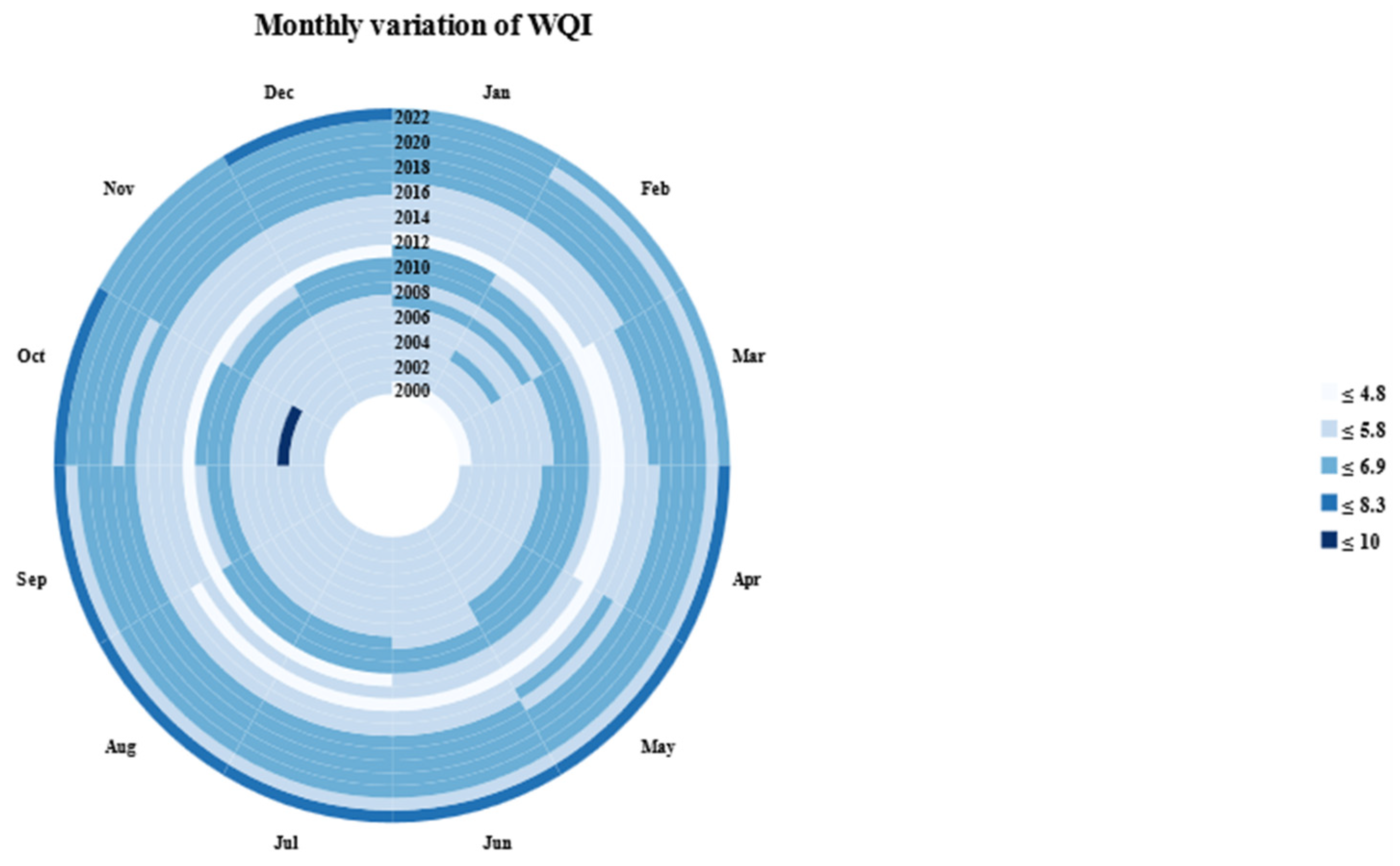
3.3. Monthly Variation of WQI

The data clock visualisations in this study illustrate the monthly variations in the WQI over a span of 22 years (Figure 6, Figure 7 and Figure 8). The years are marked along the inner edge of the concentric rings, while the months are plotted along the outer edge. The WQI values are represented in five different coloured bins. The WQI range in the Cooby Reservoir varies from 15.31 to 50, in Cressbrook Reservoir from 5.9 to 18 and in Perseverance Reservoir from 4.8 to 10 throughout the data period. According to the WQI values as discussed in Table 2, the water quality in all three reservoirs is described as Poor and Very Poor. The water quality in Cooby Reservoir is better in comparison with the other two. From the figures, it is evident that the water quality tends to be relatively better during the months of April and May across all three reservoirs.

3.4. Performance Comparison of Machine Learning and Deep Learning Models

In this study, a combination of four machine learning (ML) algorithms and two deep learning (DL) algorithms were utilised to predict the WQI of the three dam reservoirs. The ML algorithms used were Random Forest Regressor (RFR), Support Vector Regressor (SVR), AdaBoost Regressor and XGBoost Regressor. Two DL algorithms, namely BiLSTM and GRU were used. These regression algorithms utilised five water quality parameters and were tested using 22 years of weekly data. Typically, across the training and testing phases, models undergo evaluation through a comparison of observed data and simulated data points. Model accuracy was assessed utilising seven accuracy metrices as detailed in Table 5, Table 6 and Table 7. This evaluation encompasses the model’s performance in both the training and testing phases.
In the case of Cooby Reservoir, the prediction of the WQI using the proposed machine learning and deep learning algorithms yielded notably elevated R2 values of 0.99, excluding the BiLSTM model (0.91). The results depict that the model’s projected values exhibited notably close proximity to 1 during both the training and testing phases. For RMSE, SVR yielded the most minimal outcomes (1.22) during the training phase. AdaBoost and XGBoost delivered moderate RMSE performance outcomes (0.871, 0.55, 0.1752). Among the statistical metrics, MAPE demonstrated the least favorable performance (6.895, 1.48, 3.535, 3.58) within the SVR and AdaBoost models, while in Perseverance Reservoir it also showed lower performance in the AdaBoost (1.1601, 1.1543) and BiLSTM models (1.119, 1.232). Secondly, pertaining to Cressbrook Reservoir, the R2 value is 0.99 for all proposed models apart from the BiLSTM model which yielded a value of 0.89 associated with the RMSE value (1.404 and 1.494) in the training and testing phases, respectively. MAPE exhibited the least favorable performance (1.2027, 1.221, 1.033, 1.111) in the context of the AdaBoost and BiLSTM models.
Moreover, mirroring this trend, within the Perseverance Reservoir, R2 values performed well across all models except for the BiLSTM. Concurrently, other accuracy metrics yielded favorable outcomes, barring the instance of MAPE exceeding 1 in both the AdaBoost and BiLSTM scenarios. Of utmost significance, the Coefficient of Efficiency (CE), Willmott Index (d) and MSRE exhibited exceptional precision in predicting the WQI in both phases for all three reservoirs.

3.5. Comparison of Results by Radar Graph

Radar charts, also known as radar graphs, are graphical representations that display orthogonal coordinate axes into non-orthogonal coordinate axes within a circular layout. They are particularly useful for comparing multiple variables across distinct categories or entities. Radial charts are particularly useful for visualising multi-dimensional data and showcasing the interrelation between them on a two-dimensional plane. The radial coordinate axes intersect at the center of the circle [73]. It is a useful tool to represent multivariate data, and for this reason, it is simpler when associated with statistical analyses [74]. In this study, radar charts were created using Microsoft Excel to illustrate the performance of six different algorithms in predicting the WQI of the three dam reservoirs. Figure 9, Figure 10 and Figure 11 show these radar plots depicting the values of seven metrices for each algorithm. The radar charts provide a clear and concise visual representation of the performance of the algorithms allowing for easy comparison and evaluation.
Upon scrutinising the radar plots of accuracy metrices for the three reservoirs, some key observations can be synthesised as follows:
  • For the Cooby Reservoir charts (Figure 9), the R2 values prominently reach 0.99, demonstrating the robust predictive capabilities of the models. Remarkably, this high accuracy is maintained consistently except for the BiLSTM model, signifying its comparative deviation. The RMSE and MAE values align well with the R2 results, remaining relatively low, further underscoring the models’ proficiency. There is some deviation in the MAPE value in the case of the SVR and AdaBoost models.
  • In the context of the Cressbrook Reservoir (Figure 10), the radar charts accentuate a trend that closely mirrors the Cooby Reservoir results. Once again, the models yield impressive R2 values near 0.99, underscoring their accuracy in predicting water quality.
  • The radar charts for Perseverance Reservoir (Figure 11) offer insights parallel to those of the Cooby and Cressbrook Reservoirs.
  • The Coefficient of Efficiency (CE) and Willmott Index (d) continue to shine as indicators of an impressive match between observed and simulated data, substantiating the models’ reliability for all three reservoirs.

4. Discussion

Water quality data show a non-linear distribution and assessing the quality of water bodies traditionally involves time-consuming field data collection and extensive laboratory analysis. Typically, traditional WQI analysis considers a selection of 10 to 25 parameters. However, there is a research gap in investigating the impact of climate extremes on water quality and identification of the specific parameters that are affected.
This study took into consideration the parameters influenced by runoff in order to calculate the WQI, focusing on their sensitivity to climate extremes. Upon examining the WQI over a 22-year period across various seasons and months, a noticeable pattern emerges. Water quality deteriorates during periods of extreme rainfall events. To predict the WQI accurately, the study explored the application of both machine learning and deep learning models, achieving an impressive accuracy of nearly 99%. This novel approach enhances the understanding of how climate extremes influence water quality and enables the identification of key parameters in this context.
However, it is important to note certain limitations. Data availability, especially for extreme events, may impact the models’ robustness. Moreover, while machine learning and deep learning models offer remarkable predictive capabilities, they depend on historical patterns and may not fully capture unpredictable events.
Despite the limitations, this study incorporated the use of ESRI ArcGIS Pro, a Geographic Information System (GIS) software, for the first time in water quality research. ArcGIS Pro enabled the visualisation and analysis of spatial data, allowing for a comprehensive assessment of the status and variation of the WQI. The outcomes generated by ArcGIS Pro can be conveniently uploaded to the web, providing accessible information for users to monitor and comprehend water quality status.
Moving forward, potential developments include expanding the range of variables considered, refining model algorithms and incorporating dynamic modelling to provide a clearer understanding of water dynamics. This comprehensive approach aligns seamlessly with the broader aim of sustainable water resource management.

5. Conclusion and Future Works

Water is one of the most predominant natural resources on earth because all of life depends on it. Different governments, non-government, industrial and academic institutions are working for the protection and sustainability of this resource. Water quality prediction is crucial to ensure the proper management of potable water sources and it can also narrow down the detrimental effects arising from poor water quality. Data collection for water quality indicators is now becoming accessible and manageable due to advanced technologies. Efficient analysis of these data to provide constructive guidelines and warnings is a big challenge. The management of regional and remote water services under extreme weather conditions faces new challenges as a result of the increasing number of these events. The ability to recognise the cause and time of pollution may ease the challenges for water supply authorities to act in accordance with this and effect-based solutions can deliver explanatory information to policymakers.
This study explored the ability of four machine learning and two deep learning models used in the prediction of the WQI with five input parameters that are affected due to extreme rainfall. All the models are evaluated using seven accuracy measures. This study shows that XGBoost and GRU yielded the highest accuracy, showcasing an R2 value of 0.99. Conversely, the Bidirectional LSTM (BiLSTM) deep learning model demonstrated moderate accuracy, with results ranging from 88% to 90% for water quality prediction across all reservoirs. The results of this research offer a valuable contribution to the development of a rapid and cost-effective water quality monitoring system that can be integrated with climate extremes. By leveraging the power of machine learning, deep learning and GIS technologies, this study contributes to the advancement of efficient and accurate water quality assessment and management in the face of changing climate conditions.
There is an opportunity to translate these findings into practical applications. Developing a real-time monitoring system that integrates the predictive models could enable water authorities to respond swiftly to fluctuations in water quality due to climate extremes. This could aid in implementing timely mitigation measures and ensuring a safe water supply.
To further enrich the accuracy and applicability of the models, incorporating more meteorological data, land-use patterns and pollution sources could provide a more comprehensive understanding of the factors impacting water quality. This holistic approach would enable a more accurate representation of the interconnection between climate extremes and water quality.
In our future work, we will apply other advanced technology and remote sensing techniques to monitor and predict water quality. In addition to this, we will observe the trends and patterns of rainfall over extended periods to examine how water bodies respond to evolving climate conditions, facilitating proactive management strategies. Our work will guide water managers and policymakers in their efforts to prepare for dealing with extreme events through early warning.

Author Contributions

Conceptualization: S.Z.F.; data collection and compilation: S.Z.F.; methods and analysis: S.Z.F.; writing—original draft preparation: S.Z.F.; writing—review and editing: D.R.P., M.J.A. and S.C.; supervision: D.R.P., M.J.A. and S.C. All authors have read and agreed to the published version of the manuscript.

Funding

This research received no external funding.

Acknowledgments

The authors would like to thank the TRC for providing the water quality data. This research has been supported by the Graduate Research School, University of Southern Queensland and this is a part of the first author’s Ph.D. project entitled “An Integrated Spatial Decision Support Framework for Monitoring and Management of Surface Water Quality Influenced by Climate Change”.

Conflicts of Interest

The authors declare no conflict of interest.

References

  1. Wu, D.; Wang, H.; Seidu, R. Smart data driven quality prediction for urban water source management. Future Gener. Comput. Syst. 2020, 107, 418–432. [Google Scholar] [CrossRef]
  2. Ritchie, H.; Roser, M. Urbanisation. In Our World in Data. 2018. Available online: https://ourworldindata.org/urbanization (accessed on 9 June 2023).
  3. Bakkes, J.A.; Bosch, P.R.; Bouwman, A.F.; Eerens, H.C.; Den Elzen, M.G.J.; Isaac, M.; Janssen, P.H.M.; Goldewijk, K.K.; Kram, T.; De Leeuw, F.A.A.M.; et al. Background Report to the OECD Environmental Outlook to 2030: Overviews, Details, and Methodology of Model-Based Analysis; Netherlands Environmental Assessment Agency (MNP): Bilthoven, The Netherlands; OECD: Paris, France, 2008. [Google Scholar]
  4. Nouraki, A.; Alavi, M.; Golabi, M.; Albaji, M. Prediction of water quality parameters using machine learning models: A case study of the Karun River, Iran. Environ. Sci. Pollut. Res. 2021, 28, 57060–57072. [Google Scholar] [CrossRef] [PubMed]
  5. Xu, J.; Gao, X.; Yang, Z.; Xu, T. Trend and attribution analysis of runoff changes in the Weihe River basin in the last 50 years. Water 2021, 14, 47. [Google Scholar] [CrossRef]
  6. Alam, M.J.; Dutta, D. Predicting climate change impact on nutrient pollution in waterways: A case study in the upper catchment of the Latrobe River, Australia. Ecohydrology 2013, 6, 73–82. [Google Scholar] [CrossRef]
  7. Delpla, I.; Jung, A.-V.; Baures, E.; Clement, M.; Thomas, O. Impacts of climate change on surface water quality in relation to drinking water production. Environ. Int. 2009, 35, 1225–1233. [Google Scholar] [CrossRef]
  8. Van Vliet, M.; Zwolsman, J. Impact of summer droughts on the water quality of the Meuse river. J. Hydrol. 2008, 353, 1–17. [Google Scholar] [CrossRef]
  9. Prathumratana, L.; Sthiannopkao, S.; Kim, K.W. The relationship of climatic and hydrological parameters to surface water quality in the lower Mekong River. Environ. Int. 2008, 34, 860–866. [Google Scholar] [CrossRef]
  10. Evans, C.; Monteith, D.; Cooper, D. Long-term increases in surface water dissolved organic carbon: Observations, possible causes and environmental impacts. Environ. Pollut. 2005, 137, 55–71. [Google Scholar] [CrossRef]
  11. Zhu, Z.; Arp, P.A.; Mazumder, A.; Meng, F.; Bourque, C.P.-A.; Foster, N.W. Modeling stream water nutrient concentrations and loadings in response to weather condition and forest harvesting. Ecol. Model. 2005, 185, 231–243. [Google Scholar] [CrossRef]
  12. Zhou, Z.-Z.; Huang, T.-L.; Ma, W.-X.; Li, Y.; Zeng, K. Impacts of water quality variation and rainfall runoff on Jinpen Reservoir, in Northwest China. Water Sci. Eng. 2015, 8, 301–308. [Google Scholar] [CrossRef]
  13. Witek, Z.; Jarosiewicz, A. Long-Term Changes in Nutrient Status of River Water. Pol. J. Environ. Stud. 2009, 18, 1177–1184. [Google Scholar]
  14. Tiri, A.; Belkhiri, L.; Mouni, L. Evaluation of surface water quality for drinking purposes using fuzzy inference system. Groundw. Sustain. Dev. 2018, 6, 235–244. [Google Scholar] [CrossRef]
  15. Horton, R.K. An index number system for rating water quality. J. Water Pollut. Control Fed. 1965, 37, 300–306. [Google Scholar]
  16. Brown, R.M.; McClelland, N.I.; Deininger, R.A.; Tozer, R.G. A water quality index-do we dare. Water Sew. Work. 1970, 117, 339–343. [Google Scholar]
  17. Pesce, S.F.; Wunderlin, D.A. Use of water quality indices to verify the impact of Córdoba City (Argentina) on Suquía River. Water Res. 2000, 34, 2915–2926. [Google Scholar] [CrossRef]
  18. Khan, F.; Husain, T.; Lumb, A. Water quality evaluation and trend analysis in selected watersheds of the Atlantic region of Canada. Environ. Monit. Assess. 2003, 88, 221–248. [Google Scholar] [CrossRef]
  19. Štambuk-Giljanović, N. Water quality evaluation by index in Dalmatia. Water Res. 1999, 33, 3423–3440. [Google Scholar] [CrossRef]
  20. Abdul Hameed M Jawad, A.; Haider, S.A.; Bahram, K.M. Application of water quality index for assessment of Dokan lake ecosystem, Kurdistan region, Iraq. J. Water Resour. Prot. 2010, 2, 2715. [Google Scholar]
  21. El Osta, M.; Masoud, M.; Alqarawy, A.; Elsayed, S.; Gad, M. Groundwater suitability for drinking and irrigation using water quality indices and multivariate modeling in makkah Al-Mukarramah province, Saudi Arabia. Water 2022, 14, 483. [Google Scholar] [CrossRef]
  22. Abbasi, T.; Abbasi, S.A. Water Quality Indices; Elsevier: Amsterdam, The Netherlands, 2012. [Google Scholar]
  23. Chidiac, S.; El Najjar, P.; Ouaini, N.; El Rayess, Y.; El Azzi, D. A comprehensive review of water quality indices (WQIs): History, models, attempts and perspectives. Rev. Environ. Sci. Bio/Technol. 2023, 22, 349–395. [Google Scholar] [CrossRef]
  24. Uddin, M.G.; Nash, S.; Olbert, A.I. A review of water quality index models and their use for assessing surface water quality. Ecol. Indic. 2021, 122, 107218. [Google Scholar] [CrossRef]
  25. Lumb, A.; Sharma, T.; Bibeault, J.-F. A review of genesis and evolution of water quality index (WQI) and some future directions. Water Qual. Expo. Health 2011, 3, 11–24. [Google Scholar] [CrossRef]
  26. Dadolahi-Sohrab, A.; Arjomand, F.; Fadaei-Nasab, M. Water quality index as a simple indicator of watersheds pollution in southwestern part of I ran. Water Environ. J. 2012, 26, 445–454. [Google Scholar] [CrossRef]
  27. Kannel, P.R.; Lee, S.; Lee, Y.-S.; Kanel, S.R.; Khan, S.P. Application of water quality indices and dissolved oxygen as indicators for river water classification and urban impact assessment. Environ. Monit. Assess. 2007, 132, 93–110. [Google Scholar] [CrossRef] [PubMed]
  28. Sutadian, A.D.; Muttil, N.; Yilmaz, A.G.; Perera, B. Development of river water quality indices—A review. Environ. Monit. Assess. 2016, 188, 1–29. [Google Scholar] [CrossRef]
  29. Ma, Z.; Li, H.; Ye, Z.; Wen, J.; Hu, Y.; Liu, Y. Application of modified water quality index (WQI) in the assessment of coastal water quality in main aquaculture areas of Dalian, China. Mar. Pollut. Bull. 2020, 157, 111285. [Google Scholar] [CrossRef]
  30. Chen, K.; Chen, H.; Zhou, C.; Huang, Y.; Qi, X.; Shen, R.; Liu, F.; Zuo, M.; Zou, X.; Wang, J.; et al. Comparative analysis of surface water quality prediction performance and identification of key water parameters using different machine learning models based on big data. Water Res. 2020, 171, 115454. [Google Scholar] [CrossRef]
  31. Chen, H.; Yang, J.; Fu, X.; Zheng, Q.; Song, X.; Fu, Z.; Wang, J.; Liang, Y.; Yin, H.; Liu, Z.; et al. Water Quality Prediction Based on LSTM and Attention Mechanism: A Case Study of the Burnett River, Australia. Sustainability 2022, 14, 13231. [Google Scholar] [CrossRef]
  32. Malek, N.H.A.; Yaacob, W.F.W.; Nasir, S.A.M.; Shaadan, N. Prediction of Water Quality Classification of the Kelantan River Basin, Malaysia, Using Machine Learning Techniques. Water 2022, 14, 1067. [Google Scholar] [CrossRef]
  33. Ahmed, U.; Mumtaz, R.; Anwar, H.; Shah, A.A.; Irfan, R.; García-Nieto, J. Efficient water quality prediction using supervised machine learning. Water 2019, 11, 2210. [Google Scholar] [CrossRef]
  34. Tung, T.M.; Yaseen, Z.M. A survey on river water quality modelling using artificial intelligence models: 2000–2020. J. Hydrol. 2020, 585, 124670. [Google Scholar]
  35. Deka, P.C. Support vector machine applications in the field of hydrology: A review. Appl. Soft Comput. 2014, 19, 372–386. [Google Scholar]
  36. Sengorur, B.; Koklu, R.; Ates, A. Water quality assessment using artificial intelligence techniques: SOM and ANN—A case study of Melen River Turkey. Water Qual. Expo. Health 2015, 7, 469–490. [Google Scholar] [CrossRef]
  37. Xu, T.; Coco, G.; Neale, M. A predictive model of recreational water quality based on adaptive synthetic sampling algorithms and machine learning. Water Res. 2020, 177, 115788. [Google Scholar] [CrossRef] [PubMed]
  38. Lutins, E. Ensemble Methods in Machine Learning: What Are They and Why Use Them? Available online: https://towardsdatascience.com/ensemble-methods-in-machine-learning-what-are-they-and-why-use-them (accessed on 8 June 2023).
  39. Lu, H.; Ma, X. Hybrid decision tree-based machine learning models for short-term water quality prediction. Chemosphere 2020, 249, 126169. [Google Scholar] [CrossRef]
  40. Chen, L. Basic Ensemble Learning (Random Forest, AdaBoost, Gradient Boosting)-Step by Step Explained. Available online: https://towardsdatascience.com/basic-ensemble-learning-random-forest-adaboost-gradient-boosting-step-by-step-explained (accessed on 8 June 2023).
  41. Masui, T. All You Need to Know about Gradient Boosting Algorithm. Available online: https://towardsdatascience.com/all-you-need-to-know-about-gradient-boosting-algorithm (accessed on 8 June 2023).
  42. Aldhyani, T.H.; Al-Yaari, M.; Alkahtani, H.; Maashi, M. Water quality prediction using artificial intelligence algorithms. Appl. Bionics Biomech. 2020, 2020, 6659314. [Google Scholar] [CrossRef]
  43. Chen, Z.; Xu, H.; Jiang, P.; Yu, S.; Lin, G.; Bychkov, I.; Hmelnov, A.; Ruzhnikov, G.; Zhu, N.; Liu, Z. A transfer Learning-Based LSTM strategy for imputing Large-Scale consecutive missing data and its application in a water quality prediction system. J. Hydrol. 2021, 602, 126573. [Google Scholar] [CrossRef]
  44. Sugandhi, A. What Is Long Short Term Memory (LSTM)—Complete Guide. Knowledge Hut. Available online: https://www.knowledgehut.com/blog/web-development/long-short-term-memory (accessed on 8 June 2023).
  45. Zhou, J.; Chu, F.; Li, X.; Ma, H.; Xiao, F.; Sun, L. Water quality prediction approach based on t-SNE and SA-BiLSTM. In Proceedings of the 2020 IEEE 22nd International Conference on High Performance Computing and Communications; IEEE 18th International Conference on Smart City; IEEE 6th International Conference on Data Science and Systems (HPCC/SmartCity/DSS), Yanuca Island, Fiji, 14–16 December 2020; IEEE: Piscataway, NJ, USA, 2020; pp. 708–714. [Google Scholar]
  46. Kostadinov, S. Understanding GRU Networks. Towards Data Science. Available online: https://towardsdatascience.com/understanding-gru-networks (accessed on 9 June 2023).
  47. Xu, J.; Wang, K.; Lin, C.; Xiao, L.; Huang, X.; Zhang, Y. FM-GRU: A Time Series Prediction Method for Water Quality Based on seq2seq Framework. Water 2021, 13, 1031. Available online: https://www.mdpi.com/2073-4441/13/8/1031 (accessed on 9 June 2023). [CrossRef]
  48. Miles, K.; Byrnes, J.; Bannon, K. Review of Regional Water Quality and Security, Review and Reform Strategy; Infrastucture Australia; AECOM Australia Pty Ltd.: Sydney, Australia, 2010; Volume 1. [Google Scholar]
  49. Wyrwoll, P.R.; Manero, A.; Taylor, K.S.; Rose, E.; Quentin Grafton, R. Measuring the gaps in drinking water quality and policy across regional and remote Australia. NPJ Clean Water 2022, 5, 32. [Google Scholar] [CrossRef]
  50. T. R. Council. Where Our Water Comes from. TRC. Available online: https://www.tr.qld.gov.au/environment-water-waste/water-supply-dams/dams-bores/13244-where-our-water-comes-from (accessed on 9 June 2023).
  51. Climate Data Org. Toowoomba Climate, (Australia). Available online: https://en.climate-data.org/oceania/australia/queensland/toowoomba-66/ (accessed on 9 June 2023).
  52. Amos, M.; Baxter, G.; Finch, N.; Lisle, A.; Murray, P. I just want to count them! Considerations when choosing a deer population monitoring method. Wildl. Biol. 2014, 20, 362–370. [Google Scholar] [CrossRef]
  53. Department of Environment and Heritage Protection. Queensland Water Quality Guidelines (2009), Version 3; Queensland Government: Brisbane, Australia, 2009; ISBN 978-0-9806986-0-2.
  54. EOS Project Science Office. NASA Earth Observationory, (N.E.O)-Chlorophyll. NASA. Available online: https://earthobservatory.nasa.gov/global-maps/MY1DMM_CHLORA (accessed on 12 June 2023).
  55. Calvert Marine Museum, Using your Secchi Disk. Available online: https://www.calvertmarinemuseum.com/293/Using-Your-Secchi-Disc (accessed on 12 June 2023).
  56. Rusydi, A.F. Correlation between conductivity and total dissolved solid in various type of water: A review. In IOP Conference Series: Earth and Environmental Science; IOP Publishing: Bristol, UK, 2018; Volume 118, p. 012019. [Google Scholar]
  57. Singh, A.K.; Sathya, M.; Verma, S.; Jayakumar, S. Spatiotemporal variation of water quality index in Kanwar wetland, Begusarai, India. Sustain. Water Resour. Manag. 2020, 6, 1–8. [Google Scholar] [CrossRef]
  58. Cotruvo, J.A. WHO guidelines for drinking water quality: First addendum to the fourth edition. J.-Am. Water Work. Assoc. 2017, 109, 44–51. [Google Scholar] [CrossRef]
  59. Esri. Chart. Available online: https://pro.arcgis.com/en/pro-app/3.0/help/analysis/geoprocessing/charts (accessed on 7 June 2023).
  60. Bureau of Meteorology. Climate Glossary. BOM. Available online: http://www.bom.gov.au/climate/glossary/seasons.shtml (accessed on 13 June 2023).
  61. Gnauck, A. Interpolation and approximation of water quality time series and process identification. Anal. Bioanal. Chem. 2004, 380, 484–492. [Google Scholar] [CrossRef] [PubMed]
  62. Swetha, P.; Rasheed, A.H.K.; Harigovindan, V. Random Forest Regression based Water Quality Prediction for Smart Aquaculture. In Proceedings of the 2023 4th International Conference on Computing and Communication Systems (I3CS), Shillong, India, 16–18 March 2023; IEEE: Piscataway, NJ, USA, 2023; pp. 1–5. [Google Scholar]
  63. Peddisetty, T. Support Vector Regression in Python. Towards Data Science. Available online: https://towardsdatascience.com/baby-steps-towards-data-science-support-vector-regression-in-python (accessed on 14 June 2023).
  64. Pedregosa, F.; Varoquaux, G.; Gramfort, A.; Michel, V.; Thirion, B.; Grisel, O.; Blondel, M.; Prettenhofer, P.; Weiss, R.; Dubourg, V.; et al. Scikit-learn: Machine Learning in Python. J. Mach. Learn. Res. 2011. Available online: https://scikit-learn.org/stable/modules/ensemble.html#adaboost (accessed on 15 June 2023). [CrossRef]
  65. Chen, T.; Guestrin, C. Xgboost: A scalable tree boosting system. In Proceedings of the 22nd ACM SIGKDD International Conference on Knowledge Discovery and Data Mining, San Francisco, CA, USA, 13–17 August 2016; pp. 785–794. [Google Scholar]
  66. Kang, H.; Yang, S.; Huang, J.; Oh, J. Time series prediction of wastewater flow rate by bidirectional LSTM deep learning. Int. J. Control Autom. Syst. 2020, 18, 3023–3030. [Google Scholar] [CrossRef]
  67. Zhang, Y.-g.; Tang, J.; He, Z.-y.; Tan, J.; Li, C. A novel displacement prediction method using gated recurrent unit model with time series analysis in the Erdaohe landslide. Nat. Hazards 2021, 105, 783–813. [Google Scholar] [CrossRef]
  68. Nagelkerke, N.J. A note on a general definition of the coefficient of determination. Biometrika 1991, 78, 691–692. [Google Scholar] [CrossRef]
  69. Singh, A.; Singh, R.; Kumar, A.S.; Kumar, A.; Hanwat, S.; Tripathi, V. Evaluation of soft computing and regression-based techniques for the estimation of evaporation. J. Water Clim. Chang. 2021, 12, 32–43. [Google Scholar] [CrossRef]
  70. Heddam, S. Use of optimally pruned extreme learning machine (OP-ELM) in forecasting dissolved oxygen concentration (DO) several hours in advance: A case study from the Klamath River, Oregon, USA. Environ. Process. 2016, 3, 909–937. [Google Scholar] [CrossRef]
  71. Willmott, C.J.; Ackleson, S.G.; Davis, R.E.; Feddema, J.J.; Klink, K.M.; Legates, D.R.; O’donnell, J.; Rowe, C.M. Statistics for the evaluation and comparison of models. J. Geophys. Res. Ocean. 1985, 90, 8995–9005. [Google Scholar] [CrossRef]
  72. Rowe, W. Mean Square Error & R2 Score Clearly Explained. BMC. Available online: https://www.bmc.com/blogs/mean-squared-error-r2-and-variance-in-regression-analysis (accessed on 15 June 2023).
  73. Tang, T.; Wang, S.; Wang, Z.; Chen, Y.; Wen, Y. Data-Driven Comprehensive Evaluation Model Based on the Radar Chart for the Operating State of XLPE Cables. In Proceedings of the 2022 4th Asia Energy and Electrical Engineering Symposium (AEEES), Chengdu, China, 25–28 March 2022; IEEE: Piscataway, NJ, USA, 2022; pp. 644–649. [Google Scholar]
  74. Saary, M.J. Radar plots: A useful way for presenting multivariate health care data. J. Clin. Epidemiol. 2008, 61, 311–317. [Google Scholar] [CrossRef] [PubMed]
Figure 1. Map of study area.
Geosciences 13 00293 g001
Figure 2. Support vector regression [63].
Geosciences 13 00293 g002
Figure 3. Seasonal variation of WQI of Cooby Reservoir.
Geosciences 13 00293 g003
Figure 4. Seasonal variation of WQI of Cressbrook Reservoir.
Geosciences 13 00293 g004
Figure 5. Seasonal variation of WQI of Perseverance Reservoir.
Geosciences 13 00293 g005
Figure 6. Monthly variation of WQI of Cooby Reservoir.
Geosciences 13 00293 g006
Figure 7. Monthly variation of WQI of Cressbrook Reservoir.
Geosciences 13 00293 g007
Figure 8. Monthly variation of WQI in Perseverance Reservoir.
Geosciences 13 00293 g008
Figure 9. Radar plots for accuracy metrices of WQI prediction of Cooby Reservoir.
Geosciences 13 00293 g009aGeosciences 13 00293 g009b
Figure 10. Radar plots for accuracy metrices of WQI prediction of Cressbrook Reservoir.
Geosciences 13 00293 g010
Figure 11. Radar plots for accuracy metrices of WQI prediction of Perseverance Reservoir.
Geosciences 13 00293 g011
Table 1. Parameters with their standard limits (QWQG) and weightage [53].
ParameterStandard LimitsWeighting ValueRelative Weight
pH6.5–8.540.19
TDS500 mg/L40.19
Turbidity5 NTU30.14
Ammonia Nitrogen0.550.24
Phosphate0.005 to 0.05 mg/L
Generally, less than 0.03 mg/L
50.24
Sum = 1
Table 2. Water quality class and use [57].
WQIClassWater QualityTreatment and Application
90–100IExcellentWater treatment not required. Can be utilised for protection of ecosystem.
70–90IIGoodPre-treatment is necessary. After the treatment, suitable for human use and ecosystem conservation.
50–70IIIMediumCan be applied for agricultural purposes. Not suitable for human use.
25–50IVPoorSubstantial treatment is required before any use. Not fit for human use.
0–25VVery PoorNot suitable for any kind of consumption. Only usage is for navigation or transportation on water.
Table 3. Accuracy metrices.
NamePurposeValue
Coefficient of Determination (R2)Measure of variance of regression model. Measures the ability to predict the dependent variable from independent variable [68]. More than 0.90 indicates good fit of data.
Root Mean Squared Error (RMSE)Measures the deviation between actual and predicted values [69].Zero value indicates perfect fit. The lower the value, the closer to perfect the estimation.
Mean Absolute Error (MAE)Estimates the mean absolute error between the actual and predicted values [70]. A lower value close to zero indicates higher accuracy.
Mean Absolute Percentage Error (MAPE)Indicates how far the predictions are from average. It measures the average magnitude of error in a model [70]. A value closer to zero indicates better predictions.
Coefficient of Efficiency (CE)Compares the relative performance of residual variance with initial variance [69]. CE > 0.90—complete appropriate simulation.
0.90 > CE > 0.60—appropriate simulation.
CE < 0.60—inappropriate simulation
Index of Agreement, Willmott Index (d)Measures how the model estimates the simulated actual data [71]. Zero indicates no match; one indicates ideal match.
Mean Squared Relative Error (MSRE)Mean of square of errors [72]. Closer it is to 0, the closer to perfect the prediction.
Table 4. Descriptive statistics of the variables for three reservoirs.
ReservoirVariablePhosphateTurbiditypHN_NH3_FIATDSWQI
CoobyMean0.0059604.2632578.3121660.004962621.3627723.670963
Std0.02364430.1035670.4331220.015783269.1674110.253997
Min0.0000000.0000002.4000000.00000029.000001.104762
Max0.5800001025.0000009.4000000.2000001247.0000047.504762
CressbrookMean0.0110602.7155907.8639620.008916212.0523818.078186
Std0.03783414.2250740.4111650.01724936.7422441.399705
Min0.0000000.4700006.0000000.000000106.0000004.038095
Max0.950000461.0000008.9000000.075000325.00000012.380952
PerseveranceMean0.0063083.9186307.6581320.006209139.2063375.303099
Std0.0335616.6345510.3915200.01878716.9584000.646034
Min0.0000000.2700006.3800000.00000091.0000003.466667
Max1.000000106.0000008.7000000.300000185.0000007.047619
Table 5. Accuracy measures of ML and DL models for Cooby Reservoir.
AlgorithmPhaseR2RMSEMAEMAPECEdMSRE
RFRTraining0.990.07990.02170.45180.990.990.00174
Testing0.990.0480.01920.2660.990.990.000048
SVRTraining0.981.220.26966.8950.980.980.0466
Testing0.990.21270.06431.480.980.980.0020
AdaBoostTraining0.9930.8710.7063.5350.990.990.018
Testing0.9930.550.3083.580.990.990.0022
XGBoostTraining0.99990.17520.01190.06570.990.990.0000005
Testing0.99990.08160.03140.31860.990.990.000044
BiLSTMTraining0.910.2860.19690.8380.990.990.00016
Testing0.910.3390.2120.6760.990.990.00072
GRUTraining0.99990.03820.03430.14810.990.990.0000018
Testing0.99990.02710.01550.25520.90.990.0000045
Table 6. Accuracy measures of ML and DL models for Cressbrook Reservoir.
AlgorithmPhaseR2RMSEMAEMAPECEdMSRE
RFRTraining0.99970.02340.00420.04520.990.990.000002
Testing0.9990.03670.00330.03540.990.990.00002
SVRTraining0.9970.07540.05620.72030.990.990.000071
Testing0.9980.09670.02640.64940.990.990.000575
AdaBoostTraining0.9920.12210.09331.20270.990.990.000122
Testing0.9920.0850.0401.2210.990.990.00033
XGBoostTraining0.99990.001990.001380.016810.990.990.00000003
Testing0.99990.0115380.003800.111460.990.990.0000047
BiLSTMTraining0.891.4041.2111.0330.970.960.0168
Testing0.891.4941.2291.1110.970.960.0376
GRUTraining0.99990.001280.001230.025380.990.990.00000007
Testing0.99990.003970.0009690.022330.990.990.00000038
Table 7. Accuracy measures of ML and DL models for Perseverance Reservoir.
AlgorithmPhaseR2RMSEMAEMAPECEdMSRE
RFRTraining0.99990.003350.0008570.021260.990.990.0000003
Testing0.99990.005540.001820.036430.990.990.0000012
SVRTraining0.9980.04030.03640.69290.990.990.000025
Testing0.9980.03960.03590.67050.990.990.000055
AdaBoostTraining0.9880.07040.05951.16010.990.990.000083
Testing0.9880.07130.06031.15430.990.990.000191
XGBoostTraining0.99990.00110.006680.01260.990.990.000000046
Testing0.99990.008250.002040.09660.990.990.0000082
BiLSTMTraining0.890.64040.51911.1190.990.990.0188
Testing0.880.41990.2221.2320.980.990.0159
GRUTraining0.99990.03860.002970.04050.990.990.00000077
Testing0.99990.003150.0026970.033110.990.990.00000014
Disclaimer/Publisher’s Note: The statements, opinions and data contained in all publications are solely those of the individual author(s) and contributor(s) and not of MDPI and/or the editor(s). MDPI and/or the editor(s) disclaim responsibility for any injury to people or property resulting from any ideas, methods, instructions or products referred to in the content.

