Article

Soil Erosion in a British Watershed under Climate Change as Predicted Using Convection-Permitting Regional Climate Projections

by
Rossano Ciampalini
1,2,*,
Elizabeth J. Kendon
3,
José A. Constantine
1,4,
Marcus Schindewolf
5 and
Ian R. Hall
1
1
School of Earth and Environmental Sciences, Cardiff University, Cardiff CF10 3AT, UK
2
Department of Earth Sciences, University of Florence, 50121 Florence, Italy
3
Met Office, Exeter EX1 3PB, UK
4
Department of Geosciences, Williams College, Williamstown, MA 01267, USA
5
Thuringian State Institute of Agriculture, 07743 Jena, Germany
*
Author to whom correspondence should be addressed.
Geosciences 2023, 13(9), 261; https://doi.org/10.3390/geosciences13090261
Submission received: 20 July 2023 / Revised: 6 August 2023 / Accepted: 8 August 2023 / Published: 29 August 2023
(This article belongs to the Section Climate)

Abstract

:
Climate change can lead to significant environmental and societal impacts; for example, through increases in the amount and intensity of rainfall with the associated possibility of flooding. Twenty-first-century climate change simulations for Great Britain reveal an increase in heavy precipitation that may lead to widespread soil loss by rising the likelihood of surface runoff. Here, hourly high-resolution rainfall projections from a 1.5 km (‘convection-permitting’) regional climate model are used to simulate the soil erosion response for two periods of the century (1996–2009 and a 13-year future period at ~2100) in the “Rother” catchment, West Sussex, England. Modeling soil erosion with EROSION 3D, we found a general increase in sediment production (off-site erosion) for the end of the century of about 43.2%, with a catchment-average increase from 0.176 to 0.252 t ha−1 y−1 and large differences between areas with diverse land use. These results highlight the effectiveness of using high-resolution rainfall projections to better account for spatial variability in the assessment of long-term soil erosion than other current methods.

1. Introduction

Climate change is expected to impact the hydrological cycle, increasing surface runoff and flooding frequency [1,2]. However, how this will affect soil erosion remains uncertain because of the complexity of the ecosystems and the involved processes. For example, the effect of vegetation in limiting soil erosion is recognized [3,4], but its growth dynamics can change in response to atmospheric CO2 levels [5,6]. The processes involved in soil erosion are also non-linear, highly variable, and difficult to estimate [7,8].
In our opinion, which is shared by other researchers, climate is a major driver in soil erosion [2,9]. Responding to major climate modes (e.g., the El Niño-Southern Oscillation—ENSO; North Atlantic oscillation—NAO; etc.) it might contribute to regional soil erosion impacting on precipitation, soil moisture, and runoff [10,11].
Anthropic action also has a direct influence on soil erosion [12,13] that cannot be easily distinguished from the climatic component. Such action can play out directly, reducing land cover and exposing soil, improving runoff production, then erosion, and indirectly, modifying hydraulic and mechanical properties of soil favoring surface runoff [4]. The processes have been widely debated in works dealing with anthropogenic action in land degradation [12,14,15]. In addition, land management frequently acts at the same time as human-induced climate change and the records we dispose of are generally limited in space and time [16,17,18].
However, as a result of climate change, precipitation, and especially extreme events, are estimated to increase in many regions of the globe [19,20,21] with an expected impact on soil erosion as already recognized in current research [22,23,24,25,26] and in two recent reviews [27,28]. A recent report by the Intergovernmental Panel on Climate Change (IPCC) (2022) [29] summarizes the warning for Europe of a general increase in heavy rainfall and erosion, especially for the northern and central-western EU. Although the economic consequences for northern European agriculture are unclear, climatic effects on infrastructure and inland flooding are to be considered among the ongoing damages, as well as potential catastrophic erosion.
For decades, forecasting future climate change has been accomplished using global and regional climate models (GCMs—Global Climate Models and RCMs—Regional Climate Models) [30], powerful simulation tools that model the natural processes on Earth and the atmosphere [31]. One issue with the use of GCM/RCM outputs is that they have coarse spatial grids neglecting local phenomena (typically ranging from 60 to 300 km and 10–50 km); by contrast, hydrological processes usually respond to smaller scales (i.e., tens to hundreds of meters). Furthermore, typical GCMs and RCMs rely on a convective parameterization scheme to represent the average effects of convection, which leads to known deficiencies in the simulation of the diurnal cycle of rainfall and extreme precipitation events on hourly timescales [32,33]. Thus, there is a gap between future climate data available and the need for high spatiotemporal information for long-term hydrological and soil erosion modeling.
To overcome this weakness, downscaling techniques have been developed to produce outputs at a finer spatial and temporal resolution [34,35] but different methodologies can produce different results [27]. These methods are based on dynamical or statistical relationships between climatic data at various scales [36,37], and mostly on empirical relationships between large-scale atmospheric and daily or sub-daily observed local weather variables. These methods are used to infer regional or seasonal patterns and are suitable to inspect extreme phenomena [38].
Following this approach, several studies have explored soil erosion for future climatic scenarios as reported in some review articles [27,28]. For instance, Routschek et al. [39,40], applying the WETTREG-model (WETTerlagen-basierte REGionalisierungsmethode, WETTREG, statistical downscaling climate model), an empirical model, for south Germany, to locally downscale large-scale predictions accomplished with ECHAM5-OPYC3 (European Centre Hamburg Version4/Ocean on isopycnal coordinates–3, general circulation model) and obtaining rainfall at 5 min resolution for the periods 2041–2050 and 2091–2100. Pastor et al. [41] used long-term simulations for a future scenario (2041–2060) in Portugal based on the CNRM-ALADIN Regional Climate Model (RCM) projections with a quantile mapping approach to extract 5-min long-term time series. Marcinkowski et al. [42] adopted four different GCMs-RCMs projections with quantile mapping downscaling to cover the national Poland territory on a 5 km × 5 km grid for daily precipitation until the end of the century. Gianinetto et al. [43] downscaled data from GCMs using Random Cascades Method [44] with topographic and spatial bias correction in an Alpine catchment up to 2100. For the United Kingdom, Mullan [45] and Mullan et al. [46] statistically downscaled GCM results over Northern Ireland hypothesizing fixed increases for half-hour rainfall parameters. Other studies used climatic probabilistic projections such as the UKCP09 [47] with statistical downscaling, as in the case of Bussi et al. [48] or Ciampalini et al. [3] over basins of the Great Britain. Weather generators are also frequently used as an alternative method for downscaling data for soil erosion modeling as in Chen et al. [49] (i.e., GPCC, The Generator for Point Climate Change), the CLIGEN (“The CLImate GENerator”) in Fullhart et al. [50] (2020), and many other [51,52]. Lastly, in recent works at a continental scale, Borrelli et al. [22,53], inspected rainfall erosivity using 14 GCMs from the WorldClim dataset [54] downscaled at 30 arc-second (~1 km2) matching them as covariates with gauge series observations for present and future to simulate soil erosion over three Representative Concentration Pathways (RCPs) climatic scenarios, while Panagos et al. [55], compared future rainfall erosivity at 30 arc-second obtained by 19 downscaled General Circulation Models (GCMs), over three RCPs for the periods 2041–2060 and 2061–2080 using GloREDa (Global Rainfall Erosivity Database, Panagos et al. [56]) with 20 regional studies.
In general, sub-daily or hourly rainfall data are obtained using statistical downscaling for selected climatic stations. Even if based on robust statistics derived from long-term observations, there remain two weaknesses: (1) historical statistical parameters used for downscaling may not be consistently extrapolated to the future—i.e., the statistical relationships identified in the past or current climate may not remain valid for future conditions; (2) spatial rainfall extent and relationships are bypassed (i.e., even if a spatialization is applied, the method operates from observation points) despite the fact that they are essential to simulate hydrological processes.
Recent advances in climatic simulations, CPMs (Convection Permitting Models) [57,58,59], are a promising approach to providing reliable future climate projections at fine spatial and temporal scales. This state-of-the-art alternative approach in climate projections is provided by newly available high-resolution climate models (i.e., grid spacing less than 4 km). The models are termed “convection-permitting” [32,60] because they include mesoscale convective organization and larger storms, but still do not resolve smaller showers and convective plumes. In addition, the latest advances include ensembles of CPMs [57], allowing a first estimate of the uncertainty of future changes.
These simulations represent hourly rainfall in a more realistic way. Consequently, they can better capture storm dynamics and how they affect hydrological flows. This is verified in recent research where such projections are adopted to implement distributed hydrological models for studies in the UK [61], in temperate and alpine climates [62], and in south-west Africa [63], as well as semiarid areas [64]. The potentiality of this methodology is also explored in a soil erosion assessment over western Africa (Tanzania) [65] with the use of the RUSLE model (Revised Universal Soil Loss Equation) [66].
The main aim of this study is to exploit CPM projections and to explore the applicability of this methodology to improve spatiotemporal variability over the long term in soil erosion simulations. To our knowledge, such an approach is adopted for the first time with the use of an event-based soil erosion model investigating the impact of future climate change, here, applied to a British catchment, the Rother. All the simulations use rainfall projections from Kendon et al. [67], a multi-year simulation (13 years for present-day and future period under RCP8.5 scenario) at a 1.5 km grid scale over the United Kingdom carried out at the UK Met Office [67,68,69,70]. Soil erosion was simulated with EROSION 3D [71], a field-tested, validated, process-based soil erosion model.

2. Materials and Methods
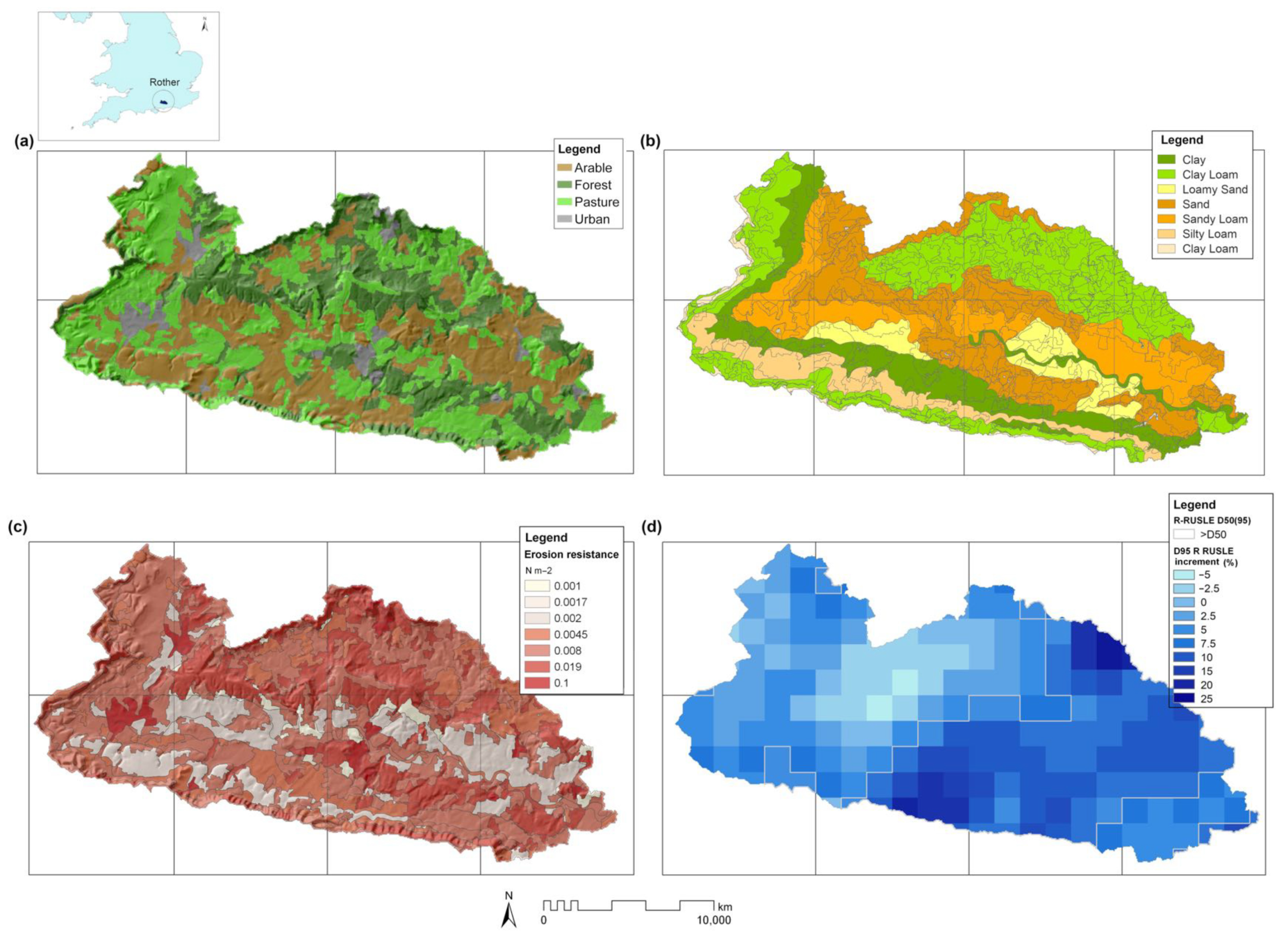
2.1. Study Area

The catchment we selected, the Rother catchment (~350 km2), is located in West Sussex in the South of England (Figure 1) and is one of the most impacted by soil erosion risk in the UK [72,73,74]. The geology of the area consists of Chalk and Lower Greensand of Cretaceous and of the paralic/continental sedimentary Wealden group. The soils developed on Cretaceous Greensand are mainly sandy and naturally at high erosion risk because of lacking cohesive bonding [75]. Within the catchment are known 21 soil associations [75], seven of which are classed as “moderate”–“high” soil erosion risk and cover about 64% of the catchment.
The elevation ranges from 0.4 to 250 m a.s.l., and the hilly morphology has an average slope of 7.2% with some locally steep areas. Annual average temperature range between 6.2 and 15.1 °C and average rainfall is about ∼826 mm [76]. Land use is categorized into arable land, pastures, and forests covering about 31.4, 40.3, and 25% of the area, respectively. (Table 1, Figure 1a). Crops are primarily winter wheat, with maize, salad vegetables, potatoes, and turnips [77,78].

2.2. Modelling Framework

A large catchment such as the Rother (350 km2) presents a non-negligible morphological and environmental complexity. To represent it, we used data from public agencies at a spatial resolution that we considered suitable for long-term simulations of soil processes and precipitation in terms of data availability and computational time. This was an hourly simulation for precipitation at a spatial cell size of 1.5 km and an erosion simulation at a spatial cell size of 50 m. Given the catchment area, we considered this as an acceptable compromise, allowing us to draw the mosaic of crop/grass/forest and urban, the first discriminator for flow generation of the erosion processes. Surface processes are also driven by landscape connectivity as largely shown by recent research [73]. In this study, the cell size we used did not allow for the inclusion of linear landscape elements in the model (e.g., roads, ditches, etc.). Although these elements may play a relevant role in the generation of confined flows, especially ditches and dirt roads that may provide a preferential pathway for sediment transport, we were forced to assume that connectivity is governed by topography and orography, as frequently performed, in modeling works at this scale. This representation is maintained for the two climate scenarios, present and future.
Given the large variability that can be injected into century projections, we decided to use some locked parameters, as others are very dynamically variable (i.e., rainfall in HD). For land use, we adopted a reduced-complexity representation with arable land use properties that have monthly variability (i.e., roughness, erodibility, cover) and that correspond to winter wheat in order to better focus on the relationship between erosion and erodibility from rainfall fields as the main variable we want to analyze in this study.
In this research, we used soil data from NSRI (National Soil Resources Institute) [79] at a regional scale. Soil types and soil properties were in agreement with the NATMAP spatial soil database for the UK—containing information regarding soil type and main properties for soil surface properties including organic matter and soil texture.
Agricultural areas—i.e., arable lands—are derived from Corine Land Cover (2012) [80] and were sub-categorized by texture classes (Figure 1b), while other land use such as forest, pastures, and urban, were considered to have constant parameters as grasslands and forests are potentially vegetated throughout the year, effectively limiting the influence of texture, and urban areas, because of the large man-made/remolded surfaces. For soil moisture, the area was divided into height sectors, and for each sector, the average value of the antecedent soil moisture was estimated from the Joint UK Land Environment Simulator (JULES) [81], which is initialized and running within the 1.5 km-CPM and the 12 km-RCM; it is based on a finite difference approximation of the Richards’ equation [82] and contains four soil layers with depths of 0.1, 0.25, 0.65, and 2.0 m.

2.2.1. Climate Projections

We used long-term climate simulations from the Met Office Unified Model (MetUM) at 1.5-km spatial resolution (i.e., CPM—Convection Permitting Model), spanning the south of Britain (13 years for present-day and future periods, Kendon et al. [32,67,70] driven by a 12 km-RCM, which was in turn driven by the Met Office Hadley Centre 60 km-GCM under the IPCC RCP8.5 scenario.
We adopted emission scenario RCP8.5 because it is a plausible high-end scenario, consistent with the current trajectory of emissions, and provides useful results in terms of changes if greenhouse gas emissions are not reduced. Although the most aggressive scenario, it represents a valuable tool for quantifying climatic risk, especially over near- to mid-term time horizons. RCP8.5 emissions are in close agreement with historical cumulative CO2 emissions and the best match out to mid-century under current and stated policies projecting high CO2 emissions by 2100 [83]. Furthermore, from an analytical point of view, it allows us to clearly identify the climate change signal above noise and results for lower emission scenarios can be obtained by the use of scaling techniques. Finally, even though this may not be the most likely scenario, it is still plausible and useful for adaptation planning.
The climate projections we adopted are based on the UKV, one of the several configurations of the Met Office Unified Model (UM) [84], used for both meteorological and climate applications. It solves the non-hydrostatic dynamics of the deep atmosphere with a semi-implicit, semi-Lagrangian numerical procedure [85] and includes a set of parameters to characterize land surface [86], boundary layer [87], convection [88], and cloud microphysics [89]. The UKV also includes a Smagorinsky–Lilly subgrid turbulence diffusion scheme (described in Brown et al. [90]) to represent turbulent mixing in areas such as the edges of convective updrafts.
Both the 12 km-RCM and the 60 km-GCM have the UM Global Atmosphere 3.0 configuration and have similar model physics to that in the 1.5 km model except that, at 1.5 km resolution, the convection scheme was switched off and the Smagorinsky–Lilly turbulence diffusion is applied. Gridded hourly radar data for the United Kingdom at 5 km resolution, available from the Nimrod database [91] for the period 2003–2010, were used to assess the spatial and temporal characteristics of hourly rainfall in the 1.5 and 12 km RCMs [32]. The 1.5-km RCM was free running in the interior with the model atmosphere and land surface evolving freely in response to information fed in at the lateral and sea surface boundaries. The 1.5 km RCM has been run for two 13-year periods, 1996–2009, and ~2100.

2.2.2. Soil Erosion Modeling

Soil erosion is simulated using EROSION 3D (version 3.0) [71,92,93], a physically based model simulating hillslope soil erosion and deposition processes caused by individual rainfall events, which was field calibrated for a large range of soil types and sediments. A detailed description of the model physics and its validation is given by various authors [94,95].
The runoff is estimated by an infiltration subroutine, based on a modified approach of Green and Ampt [96], integrating an empirical correction procedure and considering tillage practices, soil texture, and time after tillage, to simulate the effects of surface crusting, as the Green and Ampt-approach is limited in simulating only macropore flow. The basic assumption in the model is that the erosive impact of overland flow and rain splash is proportional to the momentum fluxes exerted by the flow and the falling droplets, respectively [71]. Conceptually, the momentum exerted by the runoff is expressed by:
ϑθ = Ωθ·Δψ·υθ
where Ωq is the mass rate of flow, Δψ is the width of the specified slope segment and υθ is the mean flow velocity, while for rain-splash the factor corresponds to:
ϑρ = Ωρ υρ
where Ωr is the mass rate of rainfall and υρ the mean fall velocity of droplets.
The soil exercises a resistance to particle detachment with a critical momentum which determines the soil erodibility such as:
ϑcrit = qcrit·Δψ·ρθ·υθ
where qcrit is the volume rate of flow at initial erosion and ρθ the fluid density. Erosion will occur if the sum of mobilizing forces acting on particles is larger than that of the resisting forces (i.e., E >1) and can be combined in a dimensionless coefficient:
E = (ϑθ + ϑρ)/ϑcrit
In general terms, erosion is limited either by the amount of sediment that can be detached from the soil surface or by the transport capacity of the overland flow; then, an erosion deposition balance is calculated for each cell at any time step.
EROSION 3D can provide long-term simulations and the temporal resolution of the model depends on the rainfall data available. The input parameters can be assigned to three main groups: relief parameters (DEM), land use and soil parameters, and precipitation parameters. Surface runoff, infiltration, erosion, and deposition are calculated for each raster-cell. Soil loss is given as total erosion by the lowest raster-cell in the catchment or as local balance to each raster cell.
To fit the model parameters, soil bulk density (BD) was determined for each soil polygonal class using pedotransfer functions for British soils focusing on the topsoil layer (0–30), which was subset into four categories of decreasing ‘disturbance’ representing mineral soil layers under ‘arable’ cultivation (Aar), short-term rotational ‘ley’ grassland (Ale), long-term ‘permanent’ managed grassland (Apg) and ‘other’ semi-natural vegetation (Aot). We used different pedotransfer functions as developed for the UK soils, respectively, for arable and grassland with different characteristics [97]:
BD [Aar] = 1—46 − 0.0254 LogClay + 0.0279 LogS—nd − 0.261 LogOrgC
BD [Ale] = 0.807 + 0.0989 LogClay + 0.106 LogS—nd − 0.215 LogOrgC
BD [Apg] = 0.999 + 0.0451 LogClay + 0.0784 LogS—nd − 0.244 LogOrgC
BD [Aot] = 0.870 + 0.0710 LogClay + 0.0930 LogS—nd − 0.254 LogOrgC
where Clay, Sand, and OrgC are fractions for clay, sand, and organic carbon, respectively.
For forest soil, we applied the pedotransfer function developed by Huntington et al. [98] for forest soils in the United Kingdom:
Log BD = −2—39 − 1.316(LogS—M) − 0.167(LogSOM)2,
with SOM, the soil organic matter fraction.
Finally, soil erodibility is calculated according to the EROSION 3D model rules detailed in the Parameter Catalog Application [99] using the above soil dataset. These rules are summarized by specific empirical relationships relying on erodibility to soil parameters at different crop growth stages such as:
ER = f (Texture, LU, FC, TIL, BD, OC, WC, SC, n)
where ER is Erosion resistance [Nm−2], LU is land use, FC field conditions, TIL is tillage implementations, BD is bulk density [kgm−3], OC is organic carbon content [%], WC is the initial water content [%], SC is soil cover [%], and n is the Manning’s hydraulic roughness [sm−1/3].

3. Results

3.1. Rainfall Erosivity

In general, most of the erosion impacting landscapes is induced by few concentrated rainfall events [100]; to quantify such an aspect, rainfall intensity, and erosivity are commonly represented by the 95th percentile (D95) [101,102]. Precipitation spatial variability is also central in erosion modeling, often neglected along with a detailed representation of the higher intensities. In this study, these features were captured by the km-scale of the CPMs projections, then compared to the resulting soil erosion.
We adopted the R-RUSLE erosivity factor—the product of kinetic energy times storm intensity cumulated over all events in a year— [66] for hourly precipitation as reported in Panagos et al. [103]. For the present-day and future periods, 1996–2009 and ~2100, the yearly D95 averages were 364.0 and 387.05 MJ mm ha−1 h−1 y−1, with an average increment in the future period of 23.05 MJ mm ha−1 h−1 y−1. Across the Rother catchment, the spatial variation of the R-RUSLE increment ranged from −5.7 to +23.4% with an average of +5.6% (Table 2a, Figure 1d). Rainfall erosivity exhibits a non-negligible spatial variability that consequently can lead to a significant effect on the geographical distribution of soil loss. By analyzing the spatial distribution of the D95 R-RUSLE variation (%) from the average over the two periods (1996–2009 and ~2100, Figure 1b), we observe that the highest increments are attained in the eastern and in the western of the catchment (Figure 1d), while smaller values or decrements occur in the center-west area.
In order to geographically compare the rainfall erosivity and the resulting soil erosion, we partitioned the basin using the median D95 R-RUSLE increment (D50D95 = +22.02 MJ mm ha−1 h−1 y−1; +5.27%) on the basis of the values above and below the median. The two areas reported average D95 R-RUSLE increments of +1.1 and +10.1%, respectively (Table 2b, Figure 1d).

3.2. Soil Erosion

Water erosion results from the action of rainfall erosivity, and its interaction with the local soil characteristics, which impacts accumulating over time. Since each simulated period is limited to 13 years, in order to assess whether the future changes are significant compared to year-to-year variability, we used bootstrapping with replacement, resampling one thousand times the average yearly sediment loss. After applying Kolmogorov–Smirnov two tails test, we found that our estimated future soil erosion increases are significantly different from present-day simulations series (D = 0.415) at p-value level < 0.01.
For the present-day period (1996–2009) (Table 3, Figure 2), the catchment average soil loss was 0.176 ± 0.048 t ha−1 y−1. Arable soils largely contributed to total erosion, with erosion rates of 0.660 ± 0.196 t ha−1 y−1, while the erosion rates of urban areas were 0.440 ± 0.070 t ha−1 y−1. In contrast, mainly sediment deposition was observed in pastures and forests, with average rates of −0.076 ± 0.022 and −0.058 ± 0.016 t ha−1 y−1, respectively. Erosion values were widely distributed, reflecting the high variability of the phenomenon. The erosion percentiles, D05, Median, and D95 values, for the whole catchment and arable land were −1.224, 0.298, and 8.231, and −0.005, 0.555, and 9.151 t ha−1 y−1, respectively, suggesting that, locally, extreme erosion can occur. Grassland and forest showed deposition values of −1.44 × 10⁻⁶, −0.169, −12.891, and −2 × 10⁻⁷, −0.253, and −13.563 t ha−1 y−1, respectively.
Given the difficulty in obtaining historical measurements for the catchment as a whole, the results of our simulations were, in general, within the ranges of the long-term measurement campaign data for cultivated soils in the area over the recent decades [72,104,105,106,107] and recently summarized [108]. Yet, despite a recent campaign to measure sediment deposition in streams [74], it remains difficult to extrapolate erosion to the whole catchment in order to compare global erosion averages over the long term. We then used the panel of measured field values available in the literature as a reference to verify that the simulated erosion is within the order of magnitude of the recorded data in the catchment area over the past decades, according to the concept of “within a reasonable convergence”. Observed data were obtained mainly surveying rilling frequency on fields, aerial photo observation on specific sites, erosion measurement on localized transects and fields, or coring sediments in rivers. Erosion in cultivated fields was very variable, with major intensity in winter and autumn, and depending on the erosive process—values ranged from little erosion for wash <0.3 m3 ha−1 y−1, as suggested for most arable soils in the UK by Evans [109], to fields with rill and gully erosion from ten to more than 100 m3 ha−1 per event [108]. Across the catchment, erosion simulations were highly influenced by land use. The greatest deposition occurred in grasslands and forests, while arable land had the highest erosion. This is corroborated by literature evidence as reported in a recent review [110] on quantifying soil erosion, runoff generating, and potential flooding mitigation effect of permanent grasslands in the UK and EU compared to arable land and forest. The works showed that permanent grassland soils generally have lower bulk density and higher hydraulic conductivity than arable soils, generating less runoff and erosion. Our results are in line (with a little underestimation in the averages) with the erosion values recorded in the country, as reported in the geodatabase ‘Soil Survey of England and Wales’ (SSEW) [111], containing 1566 records, which indicate average for the land uses arable and grassland of 1.27 and 0.72 t ha−1 y−1, respectively, and 0.00 t ha−1 y−1 for medians.
Future simulations (year ~2100) (Table 3, Figure 2) showed an increase in the average of the total soil erosion of 0.252 ± 0.097 t ha−1 y−1 with approximately a 43.2% increase in sediment delivery. Arable lands, due to their high susceptibility to water erosion and the extensive surface area (31.4%), are projected to be the major driver of the erosion increase (+40.9%, 0.930 ± 0.396 t ha−1 y−1). Conversely, grassland and forest presented an average net deposition of −0.106 ± 0.044 and −0.078 ± 0.036 t ha−1 y−1, with increases of 39.5% and 34.5%, respectively. Erosion in urban areas is expected to slightly decrease (approximately 19%, 0.354 ± 0.080 t ha−1 y−1). Furthermore, although soil erosion increased over the entire catchment, erosion rates were spatially high variable (Figure 3a). Percentiles (D05, Median, and D95) for the entire catchment, and arable land were −0.879, 0.342, and 7.969, and −1 × 10⁻⁴, 0.533, and 9.167 t ha−1 y−1, respectively. While grasslands and forests (mostly retaining sediments) were 2.1 × 10⁻⁶, −0.190, and −11.451, and −3 × 10⁻⁷, −0.241, and −11.278 t ha−1 y−1, respectively.

4. Discussion

Erosion spatial distribution is influenced by rainfall patterns and by events that generally have a limited spatial extent (i.e., hundreds of meters); the most intense rains are responsible for much of the erosion [112,113] and typically span from a few minutes to half an hour [114,115,116]. Such elements matter when assessing distributed erosion, especially for future climate scenarios. Until now, despite the downscaling procedures adopted to improve the spatial resolution, relatively coarse scale in climatic projections has been used in the current studies at catchment [3,41,48,117], regional [118,119], or larger scales [22,53,120]. Globally, such models can hardly capture the spatial variability of the processes having a more localized, sub-catchment scale extent. The introduction of CPM projections with horizontal grid spacing <4 km is a major step forward allowing to better model erosion dynamics within a catchment as confirmed in recent works on surface hydrology simulations [61,62,63].
The combined effect of the spatial patterns in rainfall erosivity and soil erodibility can lead to diversified erosion results. Our findings with long-term rainfalls indicated an increase in the D95 R-erosivity preferentially concentrated in the eastern and western area of the catchment along a SW-NE direction, with a minimum in the center-west of the catchment (Figure 1d). The most erodible soils, as labeled in the erosion resistance map based on EROSION 3D rules (i.e., clear zones and values below 0.02 N m−2 in Figure 1c), are found in horizontal bands in the southern and in the center of the catchment close to the river, corresponding to silty loam and sandy loam soils. Moreover, arable land shows large patchiness within the catchment, influencing the overall soil erosion in the area.
In order to focus on the specific impact of the rainfall, we verified the spatial matching between rainfall erosivity and the resulting soil erosion variations. The soil erosion over surfaces with D95 R-erosivity increases above and below the D50 threshold (i.e., +5.27%, areas differentiated by the blue pattern in Figure 3b) scored averages of 0.052 and 0.103 t ha−1 y−1 (+29.3% and +58.0% increases), respectively (Table 4).
We further compared the area with the largest increases in soil erosion (i.e., above the average) (Figure 3b) with the two surfaces corresponding to below, and above the D50 of the D95 R-erosivity increase. The comparison revealed that the two crossed areas covered about 16.4% and 29.7% of the catchment, respectively. The extension of the area with the highest rainfall erosivity overtakes the lower by 81.1%. This result suggests that, beyond the difference in soil erodibility and topography, usually identified as the principal driver of erosion spatial differentiation, rainfall erosivity patterns can contribute, indicating a possible benefit of using the high spatiotemporal resolution of the rainfall projections here adopted. The evidence of a specific rainfall erosivity pattern derived from this methodology is confirmed also by the results of Chapman et al. [65] that applying CPM projections for present and end of the century in West Africa (Tanzania) identified a spatial differentiation over the country between the two periods.
Plotting the two datasets (D95 R, and soil erosion increases) in a co-occurrence-density-plot (Figure 3c), we observed that, even though a significant relationship was not identified, in 68.1% of the data points, there is a positive correspondence between R-erosivity and soil erosion increase (i.e., occupying the first quadrant of the Figure 3c: RD95-R increase VS erosion increase). Such a result, despite the complexity and variability of the responses, confirms that rainfall erosivity scores and related patterns remain a major determinant of soil loss variability between the two time periods (Figure 1d and Figure 3b).
Overall, the results support the value of moving towards a detailed spatial representation of the rainfall erosivity, here captured by the high-resolution climate projections. On a future perspective, the realization of ‘CPMs ensemble projections’ (i.e., multiple climatic simulations on similar data configurations, randomly initialized), already achieved for the UK (e.g., a 12-member ensemble of UKCP Local projections, [58,121]) and Europe (e.g., multi-model CPM simulations for Europe [57,122] and a common Alpine domain, [123,124]), will allow to progress from a deterministic approach (i.e., single model realization) to more statistical methods, which will be a further advance in characterizing uncertainties in erosion modeling.

5. Conclusions

The data used in this study provide an in-depth research opportunity since the CPM high-resolution projections were employed in combination with a soil erosion model. The CPM approach avoids the need for statistical downscaling and any associated simplifications or assumptions since the climate data are provided at a more detailed spatial and temporal resolution. Modeling soil erosion with the EROSION 3D model allowed us to join the performances of a quasi-physical erosion model for soil-physics with the step-wised characteristics for the hydrological balance well incorporating the spatiotemporal variability of the rainfall data.
Following an average increase in rainfall erosivity of 5.6%, for the Rother catchment, we obtained future increases in soil loss of 43.2%.
Erosion rates are quite variable in any land use. The most reactive are cultivated areas, which show an average erosion rate variation passing from 0.66 to 0.93 t ha−1 y−1. The Median and D95 rates, in the future scenario, of 0.533 and 9.167 t ha−1 y−1, evidence the occurrence of high localized erosive intensity. This reflects the already known fact that cultivated areas are the most affected by climatic variations (i.e., more bare surface area is exposed than other land uses by months of the year). Deposition, mainly in pastures and forests, also reflects this increase, intercepting redistributed sediment more effectively.
The comparison of rainfall erosivity with the resulting erosion Increases indicated that future changes in local rainfall erosivity can drive changes in erosion and differentiate the resulting spatial pattern. Soil erosion referred to the surfaces with D95 R-erosivity increases above and below the D50 threshold scored erosion differences of +29.3% and +58.0%, respectively, confirming the impact of such spatial differentiation. This study suggests that an approach adopting high-resolution climatic data as CPMs rainfall projections can be useful to improve spatial assessment of erosion and suitable for landscape planning and protection, stockholders, and decision making, especially in future scenarios.

Author Contributions

J.A.C., E.J.K. and R.C. conceived the study. R.C. compiled baseline data and conducted model simulations. E.J.K. provided climatic projections, assisted in hypothesis development and expertise in climate-change. M.S. provided support for the erosion model EROSION 3D. I.R.H. contributed to the agreement of the research project and assisted in the development of the hypotheses. R.C. led data analysis and interpretation, assisted by all co-authors. R.C. drafted the paper, which was then reviewed by all co-authors. All authors have read and agreed to the published version of the manuscript.

Funding

The study was supported by funding from the Climate Change Consortium of Wales (C3W) for R. Ciampalini. E. J. Kendon gratefully acknowledges funding from the Joint UK BEIS/Defra Met Office Hadley Centre Climate Programme (GA01101).

Data Availability Statement

Data sharing not applicable. Data is unavailable due to privacy or ethical restrictions.

Acknowledgments

We would like to thank you all the anonymous reviewers for taking time and energy in reviewing the manuscript. We sincerely appreciate the valuable suggestions that contributed to improve the standard of the work.

Conflicts of Interest

The authors declare no conflict of interest.

References

  1. Alfieri, L.; Dottori, F.; Betts, R.; Salamon, P.; Feyen, L. Multi-Model Projections of River Flood Risk in Europe under Global Warming. Climate 2018, 6, 6. [Google Scholar] [CrossRef]
  2. IPCC—Intergovernmental Panel on Climate Change; Jia, G.; Shevliakova, E.; Artaxo, P.; De Noblet-Ducoudré, N.; Houghton, R.; House, J.; Kitajima, K.; Lennard, C.; Popp, A.; et al. Land–climate interactions. In IPCC, 2019: Climate Change and Land: An IPCC Special Report on Climate Change Desertification Land Degradation Sustainable Land Management Food Security and Greenhouse Gas Fluxes in Terrestrial Ecosystems; Shukla, P.R., Skea, J., Calvo Buendia, E., Masson-Delmotte, V., Pörtner, H.O., Roberts, D.C., Zhai, P., Slade, R., Connors, S., et al., Eds.; Cambridge University Press: Cambridge, UK; New York, NY, USA, 2019; pp. 131–247. [Google Scholar] [CrossRef]
  3. Ciampalini, R.; Constantine, J.A.; Walker-Springett, K.J.; Hales, T.C.; Ormerod, S.J.; Hall, I.R. Modelling soil erosion responses to climate change in three catchments of Great Britain. Sci. Total Environ. 2020, 749, 141657. [Google Scholar] [CrossRef] [PubMed]
  4. Durán Zuazo, V.H.D.; Rodríguez Pleguezuelo, C.R. Soil-erosion and runoff prevention by plant covers. A review. Agron Sustain Dev. 2008, 28, 65–86. [Google Scholar] [CrossRef]
  5. Arneth, A. Uncertain future for vegetation cover. Nature 2015, 524, 44–45. [Google Scholar] [CrossRef]
  6. Davies-Barnard, T.; Valdes, P.J.; Singarayer, J.S.; Wiltshire, A.J.; Jones, C.D. Quantifying the relative importance of land cover change from climate and land use in the representative concentration pathways. Glob. Biogeochem. Cycles 2015, 29, 842–853. [Google Scholar] [CrossRef]
  7. Parsons, A.J. How Reliable Are Our Methods for Estimating Soil Erosion by Water? Sci Total Environ. 2019, 676, 215–221. [Google Scholar] [CrossRef]
  8. Shanshan, W.; Baoyang, S.; Chaodong, L.; Zhanbin, L.; Bo, M. Runoff and Soil Erosion on Slope Cropland: A Review. JRE 2018, 9, 461–470. [Google Scholar] [CrossRef]
  9. IPCC—Intergovernmental Panel on Climate Change; Olsson, L.; Barbosa, H.; Bhadwal, S.; Cowie, A.; Delusca, K.; Flores-Renteria, D.; Hermans, K.; Jobbagy, E.; Kurz, W.; et al. Land Degradation. In IPCC, 2019: Climate Change and Land: An IPCC Special Report on Climate Change Desertification Land Degradation Sustainable Land Management Food Security and Greenhouse Gas Fluxes in Terrestrial Ecosystems; Shukla, P.R., Skea, J., Calvo Buendia, E., Masson-Delmotte, V., Pörtner, H.O., Roberts, D.C., Zhai, P., Slade, R., Connors, S., van Diemen, R., et al., Eds.; Cambridge University Press: Cambridge, UK; New York, NY, USA, 2019; pp. 345–436. [Google Scholar] [CrossRef]
  10. Le, T.; Ha, K.J.; Bae, D.H. Projected response of global runoff to El Niño-Southern oscillation. Environ. Res. Lett. 2021, 16, 084037. [Google Scholar] [CrossRef]
  11. Le, T.; Bae, D. Causal Impacts of El Niño-Southern Oscillation on Global Soil Moisture Over the Period 2015-2100. Eart’s Future 2022, 10, e2021EF002522. [Google Scholar] [CrossRef]
  12. Nearing, M.A.; Xie, Y.; Liu, B.; Ye, Y. Natural and anthropogenic rates of soil erosion. ISWCR 2017, 5, 77–84. [Google Scholar] [CrossRef]
  13. Vanwalleghem, T.; Gómez, J.A.; Infante Amate, J.; González de Molina, M.; Vanderlinden, K.; Guzmán, G.; Laguna, A.; Giráldez, J.V. Impact of historical land use and soil management change on soil erosion and agricultural sustainability during the Anthropocene. Anthropocene 2017, 17, 13–29. [Google Scholar] [CrossRef]
  14. Ferreira, C.S.S.; Seifollahi-Aghmiuni, S.; Destouni, G.; Ghajarnia, N.; Kalantari, Z. Soil degradation in the European Mediterranean region: Processes, status and consequences. Sci. Total Environ. 2022, 805, 150106. [Google Scholar] [CrossRef]
  15. Li, N.; Zhang, Y.; Wang, T.; Li, J.; Yang, J.; Luo, M. Have anthropogenic factors mitigated or intensified soil erosion over the past three decades in South China? J. Environ. Manag. 2022, 302 Pt B, 114093. [Google Scholar] [CrossRef]
  16. Rothacker, L.; Dosseto, A.; Francke, A.; Chivas, A.R.; Vigier, N.; Kotarba-Morley, A.M.; Menozzi, D. Impact of climate change and human activity on soil landscapes over the past 12,300 years. Sci. Rep. 2018, 8, 1–7. [Google Scholar] [CrossRef]
  17. Mullan, D.; Matthews, T.; Vandaele, K.; Barr, I.D.; Swindles, G.T.; Meneely, J.; Boardman, J.; Murphy, C. Climate impacts on soil erosion and muddy flooding at 1.5 °C vs 2 °C warming. Land Degrad. Dev. 2018, 30, 94–108. [Google Scholar] [CrossRef]
  18. Perović, V.; Kadović, R.; Djurdjević, V.; Braunović, S.; Čakmak, D.; Mitrović, M.; Pavlović, P. Effects of changes in climate and land use on soil erosion: A case study of the Vranjska Valley Serbia. Reg. Environ. Change 2019, 19, 1035–1046. [Google Scholar] [CrossRef]
  19. Giorgi, F.; Raffaele, F.; Coppola, E. The response of precipitation characteristics to global warming from climate projections. Earth Syst. Dynam. 2019, 10, 73–89. [Google Scholar] [CrossRef]
  20. Myhre, G.; Alterskjær, K.; Stjern, C.W.; Hodnebrog, Ø.; Marelle, L.; Samset, B.H.; Sillmann, J.; Schaller, N.; Fischer, E.; Schulz, M.; et al. Frequency of extreme precipitation increases extensively with event rareness under global warming. Sci. Rep. 2019, 9, 16063. [Google Scholar] [CrossRef]
  21. Seneviratne, S.I.; Nicholls, N.; Easterling, D.; Goodess, C.M.; Kanae, S.; Kossin, J.; Luo, Y.; Marengo, J.; McInnes, K.; Rahimi, M.; et al. Changes in climate extremes and their impacts on the natural physical environment. In Managing the Risks of Extreme Events and Disasters to Advance Climate Change Adaptation. A Special Report of Working Groups I and II of the Intergovernmental Panel on Climate Change; Field, C.B., Barros, V., Stocker, T.F., Qin, D., Dokken, D.J., Ebi, K.L., Mastrandrea, M.D., Mach, K.J., Plattner, G.K., Allen, S.K., et al., Eds.; Cambridge University Press: Cambridge, UK; New York, NY, USA, 2012; pp. 109–230. [Google Scholar]
  22. Borrelli, P.; Robinson, D.A.; Panagos, P.; Lugato, E.; Yang, J.E.; Alewell, C.; Wuepper, D.; Montanarella, L.; Ballabio, C. Land use and climate change impacts on global soil erosion by water (2015–2070). Proc. Natl. Acad. Sci. USA 2020, 117, 21994–22001. [Google Scholar] [CrossRef]
  23. Burt, T.; Boardman, J.; Foster, I.; Howden, N. More rain less soil: Long-term changes in rainfall intensity with climate change. Earth Surf Process Landf. 2015, 41, 563–566. [Google Scholar] [CrossRef]
  24. Mondal, A.; Khare, D.; Kundu, S.; Meena, P.K.; Mishra, P.K.; Shukla, R. Impact of climate change on future soil erosion in different slope, land use, and soil-type conditions in a part of the Narmada River Basin, India. J. Hydrol. Eng. 2015, 20, C5014003. [Google Scholar] [CrossRef]
  25. Zabaleta, A.; Meaurio, M.; Ruiz, E.; Antigüedad, I. Simulation Climate Change Impact on Runoff and Sediment Yield in a Small Watershed in the Basque Country, Northern Spain. J. Environ. Qual. 2014, 43, 235–245. [Google Scholar] [CrossRef] [PubMed]
  26. Zhang, Y.; Hernandez, M.; Anson, E.; Nearing, M.A.; Wei, H.; Stone, J.J.; Heilman, P. Modeling climate change effects on runoff and soil erosion in southeastern Arizona rangelands and implications for mitigation with conservation practices. J. Soil Water Conserv. 2012, 67, 390–405. [Google Scholar] [CrossRef]
  27. Eekhout, J.P.C.; de Vente, J. Global impact of climate change on soil erosion and potential for adaptation through soil conservation. Earth Sci Rev. 2022, 226, 103921. [Google Scholar] [CrossRef]
  28. Li, Z.; Fang, H. Impacts of climate change on water erosion: A review. Earth Sci Rev. 2016, 163, 94–117. [Google Scholar] [CrossRef]
  29. IPCC. 2022: Climate Change 2022: Impacts, Adaptation and Vulnerability. In Contribution of Working Group II to the Sixth Assessment Report of the Intergovernmental Panel on Climate Change; Pörtner, H.O., Roberts, D.C., Tignor, M., Poloczanska, E.S., Mintenbeck, K., Alegría, A., Craig, M., Langsdorf, S., Löschke, S., Möller, V., et al., Eds.; Cambridge University Press: Cambridge, UK; New York, NY, USA, 2022; 3056p. [Google Scholar] [CrossRef]
  30. Giorgi, F. Thirty years of regional climate modeling: Where are we and where are we going next? J. Geophys. Res. 2019, 124, 5696–5723. [Google Scholar] [CrossRef]
  31. Karl, T.; Trenberth, K. Modern global change. Science 2003, 302, 1719–1722. [Google Scholar] [CrossRef]
  32. Kendon, E.J.; Roberts, N.M.; Senior, C.A.; Roberts, M.J. Realism of rainfall in a very high resolution regional climate model. JCLI 2012, 25, 5791–5806. [Google Scholar] [CrossRef]
  33. Papalexiou, S.M.; Montanari, A. Global and Regional Increase of Precipitation Extremes under Global Warming. Water Resour. Res. 2019, 55, 4901–4914. [Google Scholar] [CrossRef]
  34. Giorgi, F.B.C.; Hewitson, C.; Christensen, R.F.; Jones, R.G. (Eds.) Regional Climate Information: Evaluation and Projections. Climate Change 2001: The Scientific Basis. Contribution of Working Group I to the Third Assessment Report of the Intergovernmental Panel on Climate Change; Cambridge University Press: Cambridge, UK, 2001; pp. 583–638. [Google Scholar]
  35. Trzaska, S.; Schnarr, E. A Review of Downscaling Methods for Climate Change Projections. African and Latin American Resilience to Climate Change (ARCC); Internal Report; Center for International Earth Science Information Network (CIESIN); Columbia Climate School, Columbia University: New York, NY, USA, 2014; 42p. [Google Scholar]
  36. Lee, T.; Singh, V.P. Statistical Downscaling for Hydrological and Environmental Applications; CRC Press Taylor and Francis Group: Boca Raton, FL, USA, 2019. [Google Scholar]
  37. Xu, Z.; Han, Y.; Yang, Z. Dynamical downscaling of regional climate: A review of methods and limitations. Sci. China Earth Sci. 2018, 62, 365–375. [Google Scholar] [CrossRef]
  38. Sunyer, M.A.; Madsen, H.; Ang, P.H. A comparison of different regional climate models and statistical downscaling methods for extreme rainfall estimation under climate change. Atmos. Res. 2012, 103, 119–128. [Google Scholar] [CrossRef]
  39. Routschek, A.; Schmidt, J.; Kreienkamp, F. Impact of climate change on soil erosion? A high-resolution projection on catchment scale until 2100 in Saxony/Germany. Catena 2014, 121, 99–109. [Google Scholar] [CrossRef]
  40. Routschek, A.; Schmidt, J.; Kreienkamp, F. Climate Change Impacts on Soil Erosion: A High-Resolution Projection on Catchment Scale Until 2100. Eng. Geol. Soc. Territ. 2015, 1, 135–141. [Google Scholar]
  41. Pastor, A.V.; Nunes, J.P.; Ciampalini, R.; Koopmans, M.; Baartman, J.; Huard, F.; Calheiros, T.; Le Bissonnais, Y.; Keizer, J.J.; Raclot, D. Projecting Future Impacts of Global Change Including Fires on Soil Erosion to Anticipate Better Land Management in the Forests of NW Portugal. Water 2019, 11, 2617. [Google Scholar] [CrossRef]
  42. Marcinkowski, P.; Szporak-Wasilewska, S.; Kardel, I. Assessment of soil erosion under long-term projections of climate change in Poland. J. Hydrol. 2022, 607, 127468. [Google Scholar] [CrossRef]
  43. Gianinetto, M.; Aiello, M.; Vezzoli, R.; Polinelli, F.N.; Rulli, M.C.; Chiarelli, D.; Bocchiola, D.; Ravazzani, G.; Soncini, A. Future Scenarios of Soil Erosion in the Alps under Climate Change and Land Cover Transformations Simulated with Automatic Machine Learning. Climate 2020, 8, 8. [Google Scholar] [CrossRef]
  44. Groppelli, B.; Bocchiola, D.; Rosso, R. Spatial downscaling of precipitation from GCMs for climate change projections using random cascades: A case study in Italy. Water Resour. Res. 2011, 47, W03519. [Google Scholar] [CrossRef]
  45. Mullan, D.J.; Favis-Mortlock, D.T.; Fealy, R. Addressing key limitations associated with modelling soil erosion under the impacts of future climate change. Agric. Meteorol. 2012, 156, 18–30. [Google Scholar] [CrossRef]
  46. Mullan, D. Soil erosion under the impacts of future climate change: Assessing the statistical significance of future changes and the potential on-site and off-site problems. Catena 2013, 109, 234–246. [Google Scholar] [CrossRef]
  47. UKCP09—Hadley Centre for Climate Prediction and Research. UKCP09: Probabilistic Projections Data of Climate Parameters over UK Land. Centre for Environmental Data Analysis. 2017. Available online: https://catalogue.ceda.ac.uk/uuid/31cebae359e643ca9dbd1a8d0235d6fe (accessed on 15 July 2023).
  48. Bussi, G.; Dadson, S.J.; Prudhomme, C.; Whitehead, P.G. Modelling the future impacts of climate and land-use change on suspended sediment transport in the River Thames (UK). J. Hydrol. 2016, 542, 357–372. [Google Scholar] [CrossRef]
  49. Chen, J.; Zhang, X.J.; Li, X. A Weather Generator-Based Statistical Downscaling Tool for Site-Specific Assessment of Climate Change Impacts. Trans. ASABE 2018, 61, 977–993. [Google Scholar] [CrossRef]
  50. Fullhart, A.T.; Nearing, M.A.; McGehee, R.P.; Weltz, M.A. Temporally downscaling a precipitation intensity factor for soil erosion modeling using the NOAA-ASOS weather station network. Catena 2020, 194, 104709. [Google Scholar] [CrossRef]
  51. Li, Z. A new framework for multi-site weather generator: A two-stage model combining a parametric method with a distribution-free shuffle procedure. Clim. Dyn. 2013, 43, 657–669. [Google Scholar] [CrossRef]
  52. Chen, J.; Brissette, F.P.; Zhang, X.C. A multi-site stochastic weather generator for daily precipitation and temperature. Trans ASABE 2014, 57, 1375–1391. [Google Scholar]
  53. Borrelli, P.; Ballabio, C.; Yang, J.E.; Robinson, D.A.; Panagos, P. GloSEM: High-resolution global estimates of present and future soil displacement in croplands by water erosion. Sci. Data 2022, 9, 406. [Google Scholar] [CrossRef]
  54. Fick, S.E.; Hijmans, R.J. WorldClim 2: New 1-km spatial resolution climate surfaces for global land areas. Int. J. Climatol. 2017, 37, 4302–4315. [Google Scholar] [CrossRef]
  55. Panagos, P.; Borrelli, P.; Matthews, F.; Liakos, L.; Bezak, N.; Diodato, N.; Ballabio, C. Global rainfall erosivity projections for 2050 and 2070. J. Hydrol. 2022, 610, 127865. [Google Scholar] [CrossRef]
  56. Panagos, P.; Borrelli, P.; Meusburger, K.; Yu, B.; Klik, A.; Lim, K.J.; Yang, J.E.; Ni, J.; Miao, C.; Chattopadhyay, N.; et al. Global rainfall erosivity assessment based on high-temporal resolution rainfall records. Sci. Rep. 2017, 7, 1–12. [Google Scholar] [CrossRef]
  57. Coppola, E.; Sobolowski, S.; Pichelli, E.; Raffaele, F.; Ahrens, B.; Anders, I.; Ban, N.; Bastin, S.; Belda, M.; Belusic, D.; et al. A first-of-its-kind multi-model convection permitting ensemble for investigating convective phenomena over Europe and the Mediterranean. Clim. Dyn. 2018, 55, 3–34. [Google Scholar] [CrossRef]
  58. Kendon, E.J.; Prein, A.F.; Senior, C.A.; Stirling, A. Challenges and outlook for convection-permitting climate modelling. Phil. Trans. R. Soc. A 2021, 379, 20190547. [Google Scholar] [CrossRef]
  59. Prein, A.F.; Langhans, W.; Fosser, G.; Ferrone, A.; Ban, N.; Goergen, K.; Keller, M.; Tölle, M.; Gutjahr, O.; Feser, F.; et al. A review on regional convection-permitting climate modeling: Demonstrations prospects and challenges. Rev. Geophys. 2015, 53, 323–361. [Google Scholar] [CrossRef] [PubMed]
  60. Berthou, S.; Kendon, E.J.; Chan, S.C.; Ban, N.; Leutwyler, D.; Schär, C.; Fosser, G. Pan-European climate at convection-permitting scale: A model intercomparison study. Clim. Dyn. 2018, 55, 35–59. [Google Scholar] [CrossRef]
  61. Kay, A. Differences in hydrological impacts using regional climate model and nested convection-permitting model data. Clim. Change 2022, 173, 11. [Google Scholar] [CrossRef]
  62. Schaller, N.; Sillmann, J.; Müller, M.; Haarsma, R.; Hazeleger, W.; Hegdahl, T.J.; Kelder, T.; van den Oord, G.; Weerts, A.; Whan, K. The role of spatial and temporal model resolution in a flood event storyline approach in Western Norway. Weather. Clim. Extremes 2020, 29, 100259. [Google Scholar] [CrossRef]
  63. Ascott, M.J.; Christelis, V.; Lapworth, D.J.; Macdonald, D.M.J.; Tindimugaya, C.; Iragena, A.; Finney, D.; Fitzpatrick, R.; Marsham, J.H.; Rowell, D.P. On the application of rainfall projections from a convection-permitting climate model to lumped catchment models. J. Hydrol. 2023, 617, 129097. [Google Scholar] [CrossRef]
  64. Wang, S.; Wang, Y. Improving probabilistic hydroclimatic projections through high-resolution convection-permitting climate modeling and Markov chain Monte Carlo simulations. Clim. Dyn. 2019, 53, 1613–1636. [Google Scholar] [CrossRef]
  65. Chapman, S.; Birch, C.E.; Galdos, M.V.; Pope, E.; Jemma, D.; Bradshaw, C.; Eze, S.; Marsham, J.H. Assessing the impact of climate change on soil erosion in East Africa using a convection-permitting climate model. Environ. Res. Lett. 2021, 16, 084006. [Google Scholar] [CrossRef]
  66. Renard, K.G.; Foster, G.A.; Weesies, G.A.; McCool, D.K.; Yoder, D.C. Predicting Soil Erosion by Water: A Guide to Conservation Planning with the Revised Universal Soil Loss Equation (RUSLE); Agricultural Handbook 703; US Department of Agriculture: Washington, DC, USA, 1997; p. 404. [Google Scholar]
  67. Kendon, E.J.; Roberts, N.M.; Fowler, H.J.; Roberts, M.J.; Chan, S.C.; Senior, C.A. Heavier summer downpours with climate change revealed by weather forecast resolution model. Nat. Clim. Change 2014, 4, 570–576. [Google Scholar] [CrossRef]
  68. Chan, S.C.; Kendon, E.J.; Roberts, N.M.; Fowler, H.J.; Blenkinsop, S. The characteristics of summer sub-hourly rainfall over the southern UK in a high-resolution convective permitting model. Environ. Res. Lett. 2016, 11, 094024. [Google Scholar] [CrossRef]
  69. Chan, S.C.; Kahana, R.; Kendon, E.J.; Fowler, H.J. Projected changes in extreme precipitation over Scotland and Northern England using a high-resolution regional climate model. Clim. Dyn. 2018, 51, 3559–3577. [Google Scholar] [CrossRef]
  70. Kendon, E.J.; Ban, N.; Roberts, N.M.; Fowler, H.J.; Roberts, M.J.; Chan, S.C.; Evans, J.P.; Fosser, G.; Wilkinson, J.M. Do Convection-Permitting Regional Climate Models Improve Projections of Future Precipitation Change? BAMS 2017, 98, 79–93. [Google Scholar] [CrossRef]
  71. Schmidt, J. A mathematical model to simulate rainfall erosion. Catena Suppl. 1991, 19, 101–109. [Google Scholar]
  72. Boardman, J. The value of Google Earth™ for erosion mapping. Catena 2016, 143, 123–127. [Google Scholar] [CrossRef]
  73. Boardman, J.; Vandaele, K.; Evans, R.; Foster, I.D.L. Off-site impacts of soil erosion and runoff: Why connectivity is more important than erosion rates. Soil Use Manag. 2019, 35, 245–256. [Google Scholar] [CrossRef]
  74. Evans, J.L.; Foster, I.; Boardman, J.; Holmes, N. SMART—Sediment Mitigation Actions for the River Rother UK Proc. IAHS 2017, 375, 35–39. [Google Scholar] [CrossRef]
  75. Evans, R. Soils at risk of accelerated erosion in England and Wales. Soil Use Manag. 1990, 6, 125–131. [Google Scholar] [CrossRef]
  76. Met Office: Midhurst Climate. 2014. Available online: http://www.metoffice.gov.uk/public/weather/climate/gcp6p1zhh (accessed on 15 July 2023).
  77. Boardman, J.; Favis-Mortlock, D. The significance of drilling date and crop cover with reference to soil erosion by water with implications for mitigating erosion on agricultural land in South East England. Soil Use Manag. 2014, 30, 40–47. [Google Scholar] [CrossRef]
  78. South Downs National Park Authority. Land Use in the River Rother Catchment. Ord. Surv. 2015, 100050083. [Google Scholar]
  79. NSRI (National Soil Resources Institute). Available online: http://www.landis.org.uk/data/index.cfm (accessed on 1 February 2015).
  80. Cole, B.; King, S.; Ogutu, B.; Palmer, D.; Smith, G.; Balzter, H. Corine Land Cover 2012 for the UK Jersey and Guernsey; NERC Environmental Information Data Centre (Dataset); University of Leicester: Leicester, UK, 2015. [Google Scholar] [CrossRef]
  81. Best, M.J.; Pryor, M.; Clark, D.B.; Rooney, G.G.; Essery, R.L.H.; Ménard, C.B.; Edwards, J.M.; Hendry, M.A.; Porson, A.; Gedney, N.; et al. The Joint UK Land Environment Simulator (JULES) model description-Part1: Energy and water fluxes. Geosci. Model Dev. 2011, 4, 677–699. [Google Scholar] [CrossRef]
  82. Richards, L. Capilliary conduction of liquids through porous mediums. Physics 1931, 1, 318–333. [Google Scholar] [CrossRef]
  83. Schwalm, C.R.; Glendon, S.; Duffy, P.B. RCP8.5 tracks cumulative CO2 emissions. Proc. Nat. Acad. Sci. USA 2020, 117, 19656–19657. [Google Scholar] [CrossRef] [PubMed]
  84. Cullen, M.J.P. The unified forecast/climate model. Meteorol. Mag. 1993, 122, 81–94. [Google Scholar] [CrossRef]
  85. Davies, T.; Cullen, M.J.P.; Malcolm, A.J.; Mawson, M.H.; Staniforth, A.; White, A.A.; Wood, N. A new dynamical core for the Met Office’s global and regional modelling of the atmosphere. QJR Meteorol. Soc. 2005, 131, 1759–1782. [Google Scholar] [CrossRef]
  86. Essery, R.; Pomeroy, J. Sublimation of snow intercepted by coniferous forest canopies in a climate model. In Proceedings of the Soil-Vegetation-Atmosphere Transfer Schemes and Large-Scale Hydrological Models. Proceedings of an International Symposium, Held during the Sixth IAHS Scientific Assembly, Maastricht, The Netherlands, 18–27 July 2001; pp. 343–347. [Google Scholar]
  87. Lock, A.P.; Brown, A.R.; Bush, M.R.; Martin, G.M.; Smith, R.N.B. A New Boundary Layer Mixing Scheme. Part 1: Scheme Description and Single-Column Model Tests. Mon. Wea. Rev. 2000, 128, 3187–3199. [Google Scholar] [CrossRef]
  88. Gregory, D.; Rowntree, P.R. A Mass Flux Convection Scheme with Representation of Cloud Ensemble Characteristics and Stability-Dependent Closure. MWR 1990, 118, 1483–1506. [Google Scholar] [CrossRef]
  89. Wilson, R.W.; Ballard, S.P. A microphysically based precipitation scheme for the UK Meteorological Office Unified model. Q. J. R. Meteorol. Soc. 1999, 125, 1607–1636. [Google Scholar] [CrossRef]
  90. Brown, A.R.; Derbyshire, S.; Mason, P.J. Large-eddy simulation of stable atmospheric boundary layers with a revised stochastic subgrid model. Q. J. R. Meteorol. Soc. 1994, 120, 1485–1512. [Google Scholar] [CrossRef]
  91. Golding, B.W. Nimrod: A system for generating automated very short range forecasts. Meteorol. Appl. 1998, 5, 1–16. [Google Scholar] [CrossRef]
  92. Von Werner, M. GIS-orientierte Methoden der digitalen Reliefanalyse zur Modellierung von Bodenerosion in kleinen Einzugsgebieten. Ph.D. Thesis, Freie Universität Berlin, Berlin, Germany, 1995. [Google Scholar]
  93. Von Werner, M. Erosion-3D User manual Ver. 3.0 Revision 0.88. 06.03.2003. GeoGnostics Software: Berlin, Germany, 2003. [Google Scholar]
  94. Michael, A. Anwendung des Physikalisch Begründeten Erosionsprognosemodells EROSION 2D/3D. Empirische Ansaetze zur Ableitung der Modellparameter. Ph.D. Thesis, Technische Universität Bergakademie Freiberg, Freiberg, Germany, 2000; p. 147. [Google Scholar]
  95. Schindewolf, M.; Schmidt, J. Parameterization of the EROSION 2D/3D soil erosion model using a small-scale rainfall simulator and upstream runoff simulation. Catena 2012, 91, 47–55. [Google Scholar] [CrossRef]
  96. Green, W.H.; Ampt, G.A. Studies on soil physics: Part I. The flow of air and water through soils. J. Agric. Sci. 1911, 4, 1–24. [Google Scholar]
  97. Hallett, S.; Hollis, J.; Keay, C.A. Derivation and Evaluation of a Set of Pedogenically-Based Empirical Algorithms for Predicting Bulk Density in British Soils. National Soil Resources Institute, School of Applied Science, Cranfield University. 2009. Available online: https://www.landis.org.uk (accessed on 1 February 2015).
  98. Huntington, T.G.; Johnson, C.E.; Johnson, A.H.; Siccama, T.G.; Ryan, D.F. Carbon, organic matter, and bulk density relationships in a forested spodosol. Soil Sci. 1989, 148, 380–386. [Google Scholar] [CrossRef]
  99. Michael, A.; Schmidt, J.; Schmidt, W.A. EROSION 2D/3D. A Computer Model for the Simulation of Soil Erosion by Water. Parameter Catalog Application (2D); Technische Universität Bergakademie: Freiberg, Germany, 1996; p. 169. [Google Scholar]
  100. Dotterweich, M.; Dreibrodt, S. Past land use and soil erosion processes in central Europe. PAGES News 2011, 19, 49–51. [Google Scholar] [CrossRef]
  101. Jacob, D.; Petersen, J.; Eggert, B.; Alias, A.; Christensen, O.B.; Bouwer, L.M.; Braun, A.; Colette, A.; Déqué, M.; Georgievski, G.; et al. EURO-CORDEX: New high-resolution climate change projections for European impact research. Reg. Environ. Change 2014, 14, 563–578. [Google Scholar] [CrossRef]
  102. Diodato, N.; Verstraeten, G.; Bellocchi, G. Decadal modelling of rainfall erosivity in Belgium. Land Degrad Dev. 2012, 25, 511–519. [Google Scholar] [CrossRef]
  103. Panagos, P.; Borrelli, P.; Spinoni, J.; Ballabio, C.; Meusburger, K.; Beguería, S.; Klik, A.; Michaelides, S.; Petan, S.; Hrabalíková, M.; et al. Monthly Rainfall Erosivity: Conversion Factors for Different Time Resolutions and Regional Assessments. Water 2016, 8, 119. [Google Scholar] [CrossRef]
  104. Evans, R.; Collins, A.L.; Foster, I.D.L.; Rickson, R.J.; Anthony, S.G.; Brewer, T.; Deeks, L.; Newell-Price, J.P.; Truckell, I.G.; Zhang, Y. Extent, frequency and rate of water erosion of arable land in Britain—Benefits and challenges for modelling. Soil Use Manag. 2016, 32, 149–161. [Google Scholar] [CrossRef]
  105. Boardman, J. Soil Erosion in Britain: Updating the Record. Agriculture 2013, 3, 418–442. [Google Scholar] [CrossRef]
  106. Boardman, J.; Shepheard, M.L.; Walker, E.; Foster, I.D.L. Soil erosion and risk-assessment for on- and off-farm impacts: A test case using the Midhurst area, West Sussex, UK. J. Environ. Manag. 2009, 90, 2578–2588. [Google Scholar]
  107. Shepheard, M.L. Soil Erosion and Off-Site Impacts from the Lower Greensand Soils and Arable Lands of the Rother River Valley. Master’s Thesis, Environmental Change Institute, University of Oxford, Oxford, UK, 2003. [Google Scholar]
  108. Boardman, J.; Burt, T.; Foster, I. Monitoring soil erosion on agricultural land: Results and implications for the Rother valley, West Sussex, UK. Earth Surf. Process. Landf. 2020, 45, 3931–3942. [Google Scholar] [CrossRef]
  109. Evans, R. Water erosion in British farmers’ fields- some causes, impacts, predictions. Prog. Phys. Geogr. Earth Env. 1990, 14, 199–219. [Google Scholar] [CrossRef]
  110. Milazzo, F.; Francksen, R.M.; Zavattaro, L.; Abdalla, M.; Hejduk, S.; Enri, S.R.; Pittarello, M.; Price, P.N.; Schils, R.L.M.; Smith, P.; et al. The Role of Grassland for Erosion and Flood Mitigation in Europe: A Meta-Analysis. Agric. Ecosyst. Environ. 2023, 348, 108443. [Google Scholar] [CrossRef]
  111. Benaud, P.; Anderson, K.; Evan, M.; Farrow, L.; Glendell, M.; James, M.R.; Quine, T.A.; Quinton, J.N.; Rawlins, B.; Rickson, R.J.; et al. National-scale geodata describe widespread accelerated soil erosion. Geoderma 2020, 371, 114378. [Google Scholar] [CrossRef]
  112. Nunes, J.P.; Seixas, J.; Keizer, J.J.; Ferreira, A.J.D. Sensitivity of runoff and soil erosion to climate change in two Mediterranean watersheds. Part II: Assessing impacts from changes in storm rainfall soil moisture and vegetation cover. Hydrol. Process. 2009, 23, 1212–1220. [Google Scholar] [CrossRef]
  113. Pruski, F.F.; Nearing, M.A. Runoff and soil loss responses to changes in precipitation: A computer simulation study. JSWC 2002, 57, 7–16. [Google Scholar]
  114. Dunkerley, D. Identifying individual rain events from pluviograph records: A review with analysis of data from an Australian dryland site. Hydrol. Proc. 2008, 22, 5024–5036. [Google Scholar] [CrossRef]
  115. Dunkerley, D. Rainfall intensity in geomorphology: Challenges and opportunities. Prog. Phys. Geogr. Earth Env. 2020, 45, 488–513. [Google Scholar] [CrossRef]
  116. Kampf, S.K.; Brogan, D.J.; Schmeer, S.; MacDonald, L.H.; Nelson, P.A. How do geomorphic effects of rainfall vary with storm type and spatial scale in a post-fire landscape? Geomorphology 2016, 273, 39–51. [Google Scholar] [CrossRef]
  117. Berteni, F.; Grossi, G. Water soil erosion evaluation in a small alpine catchment located in northern Italy: Potential effects of climate change. Geosciences 2020, 10, 38. [Google Scholar] [CrossRef]
  118. Maurya, S.; Srivastava, P.; Yaduvanshi, A.; Anand, A.; Petropoulos, G.; Zhuo, L.; Mall, R. Soil erosion in future scenario using CMIP5 models and earth observation datasets. J. Hydrol. 2021, 594, 125851. [Google Scholar] [CrossRef]
  119. Vantas, K.; Sidiropoulos, E.; Loukas, A. Estimating Current and Future Rainfall Erosivity in Greece Using Regional Climate Models and Spatial Quantile Regression Forests. Water 2020, 12, 687. [Google Scholar] [CrossRef]
  120. Almagro, A.; Oliveira, P.T.S.; Nearing, M.A.; Hagemann, S. Projected climate change impacts in rainfall erosivity over Brazil. Sci. Rep. 2017, 7, 8130. [Google Scholar] [CrossRef] [PubMed]
  121. Kendon, E.J.; Fischer, E.M.; Short, C.J. Variability conceals emerging trend in 100yr projections of UK local hourly rainfall extremes. Nat. Commun. 2023, 14, 1133. [Google Scholar] [CrossRef] [PubMed]
  122. Chan, S.C.; Kendon, E.J.; Berthou, S.; Fosser, G.; Lewis, E.; Fowler, H.J. Europe-wide precipitation projections at convection permitting scale with the Unified Model. Clim. Dyn. 2022, 55, 409–428. [Google Scholar] [CrossRef] [PubMed]
  123. Ban, N.; Caillaud, C.; Coppola, E.; Pichelli, E.; Sobolowski, S.; Adinolfi, M.; Ahrens, B.; Alias, A.; Anders, I.; Bastin, S.; et al. The first multi-model ensemble of regional climate simulations at kilometer-scale resolution, Part I: Evaluation of precipitation. Clim. Dyn. 2021, 57, 275–302. [Google Scholar] [CrossRef]
  124. Pichelli, E.; Coppola, E.; Sobolowski, S.; Ban, N.; Giorgi, F.; Stocchi, P.; Alias, A.; Belušić, D.; Berthou, S.; Caillaud, C.; et al. The first multi-model ensemble of regional climate simulations at kilometer-scale resolution Part 2: Historical and future simulations of precipitation. Clim. Dyn. 2021, 56, 3581–3602. [Google Scholar] [CrossRef]
Figure 1. Spatial datasets of the Rother Catchment: (a) Principal type of land use; (b) Main soil texture groups; (c) Erosion resistance parameter as calculated by the EROSION 3D model (N m −2); (d) R-RUSLE percent increases (%) over the two periods (1996–2009, and ~2100). Each cell is given the 95 percentiles (D95). Light grey line indicates the D50 bound within the dataset (+5.27%).
Geosciences 13 00261 g001
Figure 2. Model responses for present and future average erosion rates. For the whole catchment (a), and for each land use (bd), is reported the average erosion rate (y-axis) in the simulated year (x-axis) for present (1996–2009 yrs., blue lines) and future (~2100, red lines) periods. Dashed and light dashed lines represent the average values after bootstrapping resampling and ±1st.dev. bounds, respectively (values stand for erosion in (ac), and for net deposition in (d,e).
Geosciences 13 00261 g002
Figure 3. Simulation results for Rother Catchment: (a) Soil erosion increases between 1996 and 2009 and ~2100 periods; (b) Soil erosion increases above the average for low (<D50, in magenta), and high (>D50, in red) D95 R-RUSLE increases, the blue surface represents the R-RUSLE factor above the D50 for the 95-percentile distribution; (c) Density plot representing Soil erosion increase VS D95 R-RUSLE increase over the whole catchment surface.
Geosciences 13 00261 g003
Table 1. Principal type of land use, relative surface, elevation, and slope recognized over the catchment.
Land UseSurface Elevation
m. a.s.l.
Slope
%
km2%
Arable112.131.464.45.4
Grassland143.940.376.26.9
Forest89.525.087.610.2
Urban12.03.466.74.8
Total357.610075.07.2
Table 2. (a) D95 R-factor values and variation over the two periods; (b) D50 (D95) R-factor threshold and relative variation.
(a)D95 R-Factor (MJ mm ha−1 h−1 y−1)
1996–2009~2100
average364.0 ± 22.8387.0 ± 26.5
variation+23.05 (+5.6%)
D05/D50/D95327.0/363.6/405.0350.1/385.6/433.9
variation−23.1/+22.02/+28.9
(−3.76%/+5.27%/+14.88%)
(b)D95 R-factor increase (MJ mm ha−1 h−1 y−1; %)
D50 threshold+22.02; +5.27%
Subset<D50>D50
Average (%)+1.1%+10.1%
Table 3. Simulated soil erosion rates (t ha−1 y−1) after bootstrapping for the two periods (* percentiles over the global spatial dataset).
1996–2009~2100Avg. Var.
Land UseAverageSt. Dev.D05 *Med *D95 *AverageSt. Dev.D05 *Med *D95 *%
Arable0.6600.196−0.0050.5559.1510.9300.396-1 × 10−40.5339.16740.9
Grassland−0.0760.022−1.44 × 10⁻⁶−0.169−12.891−0.1060.044−2.1 × 10⁻⁶−0.190−11.45139.5
Forest−0.0580.016−2 × 10⁻⁷−0.253−13.563−0.0780.036−3 × 10⁻⁷−0.241−11.27834.5
Urban0.4400.070−0.0330.37910.7660.3540.080−0.0310.2737.958−19.5
Total0.1760.048−1.2240.2988.2310.2520.097−0.8790.3427.96943.2
Table 4. Soil erosion increases corresponding to the surfaces (above and below) defined by D50(R95) R-factor increase (Er ∩ D50(R95), on the left), and in the intersected areas of above average erosion increase and below/above D50 R-factor increase (Er avg ∩ D50(R95), on the right).
Er ∩
D50(R95)
(Erosion Incr., Value, %)
Eravg
D50(R95)
(Surface, %)
D50 R95-threshold5.27
(whole basin)
Overlapping surface
Subset<D50(R95)>D50(R95)<D50(R95)>D50(R95)
Average erosion increase0.052/+29.3%
of the whole basin
0.103/+58.0%
of the whole basin

16.4%

29.7%
Disclaimer/Publisher’s Note: The statements, opinions and data contained in all publications are solely those of the individual author(s) and contributor(s) and not of MDPI and/or the editor(s). MDPI and/or the editor(s) disclaim responsibility for any injury to people or property resulting from any ideas, methods, instructions or products referred to in the content.

