Article

Multi-Parameter Statistical Analysis of K, Th, and U Concentrations in Eastern Senegal: Implications for the Interpretation of Airborne Radiometrics

1
Laboratoire de Télédétection appliquée, Ecole Nationale Supérieure des Mines et de la Géologie, Université Cheikh Anta Diop, Dakar 5005, Senegal
2
Institut National Polytechnique Houphouët-Boigny, Yamoussoukro 1093, Côte d’Ivoire
3
Géosciences Environnement Toulouse, UMR5563 CNRS, Université de Toulouse III & IRD, 14, Avenue Edouard Belin, 31400 Toulouse, France
4
UFR des Sciences de la Terre et des Ressources Minières, Université Félix Houphouët-Boigny, Abidjan 536, Côte d’Ivoire
5
Département de Géologie, Université Cheikh Anta Diop, Dakar 5005, Senegal
*
Authors to whom correspondence should be addressed.
Geosciences 2023, 13(9), 263; https://doi.org/10.3390/geosciences13090263
Submission received: 6 February 2023 / Revised: 21 March 2023 / Accepted: 21 March 2023 / Published: 30 August 2023
(This article belongs to the Section Geochemistry)

Abstract

:
In geological mapping, maps of K, Th, and U concentrations provided by airborne radiometric surveys are widely used to delineate geological units in tropical regions from the few rare outcrops. Indeed, thanks to their specific geochemical properties and behaviors, K, Th, and U allow us to trace geological processes. However, the combination of the concentrations of these radioelements does not allow us to determine the lithology in a unique way. We examined the potential of delineating the statistical parameters of K, Th, and U concentrations for geological mapping using the purpose airborne radiometric data in eastern Senegal. The mean, standard deviation, skewness, and kurtosis were calculated and mapped at a baseline of 3000 m. We noted the narrow dispersion of skewness and kurtosis values away from the expected curve for the log-normal distribution, implying that log-normal distributions dominate at the scale of analysis. The higher moments (kurtosis and skewness) varied more over shorter distances than lower order moments (mean and standard deviation). Mixtures of log-normal distributions across some lithological contacts with large differences in statistical parameters may account for this behavior. The area covered by the airborne radiometric data was classified into eight units according to the statistical parameters. The eight clusters do not show obvious correlations with geological units, but they may be interpreted in terms of the superposition of lithology and recent superficial processes (erosion and weathering).

1. Introduction

Airborne radiometric surveys are commonly achieved for geological mapping or mineral exploration in combination with other airborne geophysical surveys, such as magnetic and electromagnetic surveys [1,2,3]. Whereas magnetic surveys document the magnetic properties of sub-surface rocks, airborne radiometrics measure the surface concentration of K, Th, and U based on the spectrum of gamma rays emitted during the decay of natural occurrences of the radioactive isotopes 40K, 232Th, 235U, and 238U, present in rocks and soils. Technically, the method relies on the use of a gamma ray detector (e.g., NaI) placed on board of an aircraft (drone, helicopter, plane) to count gamma rays and record the emission spectrum above the ground at elevations typically of several tens of meters. The intensity of the gamma rays in specific domains (counting windows) can be related to the concentrations of K, Th, and U in surface material down to a few tens of centimeters, via the application of a series of corrections to take into account the atmosphere (absorption and presence of atmospheric radon), the cosmic rays, the emissions from the aircraft itself, and the instrumental calibration [4]. The concentrations measured along the flight lines are then generally interpolated and provided as gridded maps of K, Th, and U concentrations, expressed in wt% (for K) or ppm (for U and Th). The concentrations for Th and U are generally noted eTh and eU (equivalent Th and U) to remind the fact that these concentrations are estimated under the assumption that all daughter elements of the 238U and 232Th series are in equilibrium, which may not always be the case [4,5]. During the earliest developments, airborne radiometric surveys were only used to detect radioactive anomalies corresponding to the presence of uranium deposits [6,7,8,9] or for the surveillance of nuclear sites and the mapping of potential contamination [10,11,12,13]. Nowadays, thanks to the design of new generations of more sensitive detectors, it is possible to map small variations of K, Th, and U concentrations with higher precision and resolution. Airborne radiometrics are now routinely used in regional geological mapping, in regolith mapping, or at the scale of gold exploration permits to detect and map hydrothermal alteration zones, or for prospecting low-level radioactive minerals [1,14].
Indeed, the concentrations of K, Th, and U vary widely among geological units and allow us to trace geological processes. This wide range of concentrations is due to specific geochemical properties; the three elements are strongly incompatible in silicate magmas and preferentially accumulate in silicate melts during partial melting or crystallization. The three elements also have different degrees of mobility during water-rock alteration. K is mobile, Th is generally immobile, except in very acidic conditions, and the mobility of U depends on the redox conditions during alteration processes. Mafic rocks are generally depleted in incompatible elements, which are in contrast enriched in evolved magmatic rocks, such as granite or rhyolite. Thus, in geological mapping, the concentration maps of these elements are combined with other geophysical data to delineate geological units in areas with very few outcrops [15,16,17]. Surface patterns of K concentrations may be associated with metasomatism/hydrothermalism. In regolith material or laterites, the K has been generally more or less washed out, and Th accumulates by mass balance; therefore, a map of the K/Th ratio often offers a good proxy for the occurrence of regolith [18]. K/Th ratio maps may even be combined with other remote sensing data sets in an attempt to produce automatically generated regolith maps [19]. The airborne radiometric surveys are generally represented and used as ternary maps (RGB representations with K in red, Th in green, and U in blue) or as the K/Th ratio. However, it is clear that it is impossible to determine uniquely the primary lithology and/or secondary alteration history from the sole combination of the concentrations of K, Th, and U elements [20]. The presence of regolith and soil adds further complexity to the possible relationships between K, Th, and U concentrations with different lithotypes.
Is there any way to overcome these limitations and more efficiently use the rich information comprised in radiometric surveys? Indeed, radiometric maps contain thousands or even millions of measurements of K, Th, and U concentrations. Tens or hundreds of K, Th, and U concentrations are reported at the scale of a single geological unit. This opens possibilities for statistical analyses, i.e., for the examination of the local statistical properties of K, Th, and U concentrations. This is the objective of this work, which was inspired and justified by seminal studies [20,21,22,23,24], who attempted to find universal geochemical laws of chemicals, describing the element distributions in crustal rocks for use in mineral exploration. The literature [20,21,22,23,24] showed from the first principles that various types of frequency distributions of concentrations (normal, log-normal, fractal) may be obtained from the repeated application of elementary geochemical processes to a crustal segment. Their conclusions were supported by data sets containing a relatively small number of samples (a few tens) analyzed in the laboratory. The recent work of [25] took advantage of the millions of measurements in airborne radiometrics to explore these ideas and examine the frequency distributions of K, Th, and U concentrations at various scales in the natural environment. Further analyses of radiometric data over a small region of eastern Senegal and in the Barberton granite in South Africa indicate that the frequency distributions of the concentrations of K, Th, and U have various shapes from log-normal to normal as a function of geological history and alteration processes [26,27]. For instance, changes in the statistical properties of K between the northern and southern part of the granite of Saraya have been identified and interpreted as a consequence of surface processes [26]. The frequency distributions are also scale-dependent and evolve from complex distributions (including multi-modal) to normal distributions with increasing sample size a consequence of the central limit theorem [28]. If concentrations cannot be uniquely interpreted in terms of lithology, the studies mentioned above suggest that statistical analyses may provide additional criteria to discriminate and map crustal rocks or alteration processes. For instance, the concentrations of any of the three elements within a conglomerate deposit (physical mixing) may appear much more homogeneous than in migmatites (magmatic differentiation) with complex intercalations of partial melts migrating through the rocks and melt residue at various scales. We postulate here that the statistical parameters of the concentrations at specific scale(s) may help to discriminate between one lithology and another and/or between igneous processes and secondary processes. This study represents a ”proof a concept” and proposes an approach to derive new interpretative products from airborne radiometric surveys. These new products are maps of the local statistical parameters of the frequency distributions of concentrations, considered random variables, which can be characterized by their first four moments, the expected value, the variance (or its square root, the standard deviation), the skewness, and kurtosis.
According to [23], the three first moments can be associated with particular geochemical processes, such as fractional melting, crystallization, precipitation, or dissolution. For example, frequency distributions are expected to become more and more asymmetric for higher partition coefficients. The repetition of episodes of melting also increases the standard deviation and skewness, without altering the mean value. Kurtosis is not directly discussed in these theoretical considerations [23]. Kurtosis may be directly related to skewness in log-distribution. Therefore, the calculation of kurtosis was motivated here to explore if kurtosis values would deviate significantly from the expected skew–kurtosis relationships in log-normal distributions (see Section 5.2).
The data set, covering the Eastern part of Senegal, is identical to the radiometric data already presented by [25,26]. The choice of a tropical context is justified by the fact that this approach was developed to be applied in areas where geological mapping is challenged by the limited exposure or surface rocks or the space distribution of outcrops. With respect to our previous studies in eastern Senegal [25,26], we extended this new study to the entire context of the Birimian formations of eastern Senegal. Since we had to calculate the four moments for three elements, 12 maps were generated. The dimension of this new product is too large to be easily visualized and analyzed. Therefore, we applied a classification algorithm (UMAP, standing for Uniform Manifold Approximation and Projection), which reduces the dimension of the data product. Following a classification step, we then obtained a segmented map. Following this step, we then produced a segmented map. The units of the segmented map therefore delineated boundaries between regions sharing similar statistical parameters. This map was then compared to the geological map and a map of the morphological parameter (roughness) to assess its scientific value and potential for geological mapping. The question that we addressed here was to determine whether the segmented map adds a value to the usual ternary radiometric maps to determine geological units or if it mostly reflects surface processes and the occurrence of the lateritic cover (masking therefore the geology). The first section of the manuscript focuses on the geological context of this study. The second section presents the methods for the statistical analysis, classification, and elaboration of other data sets (roughness map) and their comparison with statistical products. The third section is then devoted to identifying any relationships between the statistical parameters, the geology and topography, morphology, and roughness and to the interpretations of these relationships, with implications for geological and regolith mapping.

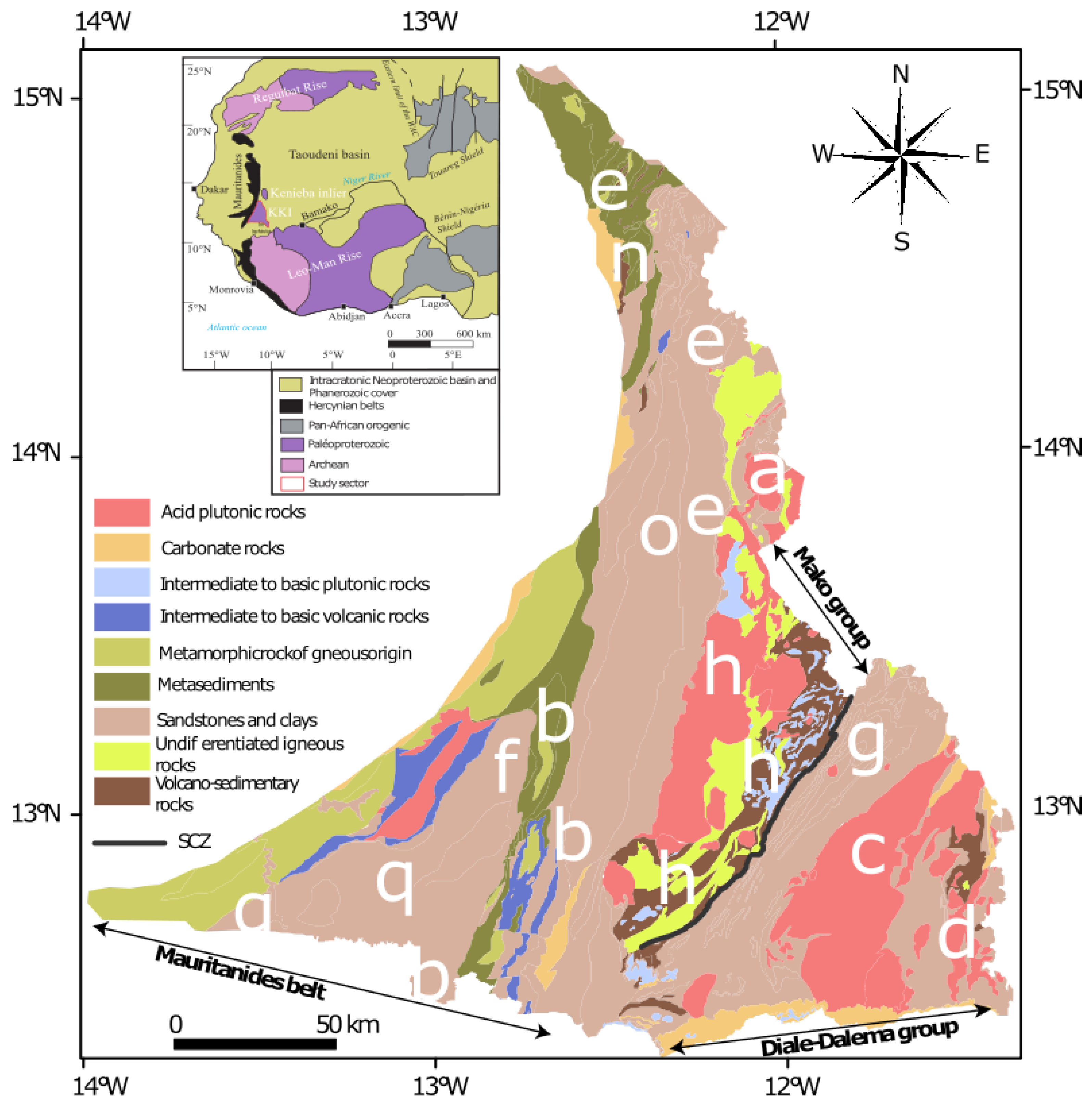
2. Geological Context

Our study area is located in southeastern Senegal, on the borders of Mali and Guinea. It contains the birimian or paleoproterozoic formations belonging to the Kedougou-Kenieba inlier of the West African Craton (Figure 1). These formations are affected by the Eburnean orogeny, which comprises two cycles: the Eburnean I cycle (2190 to 2140 Ma) [29,30,31] and the Eburnean II cycle (2120 to 2070 Ma) [32,33,34,35]. The Kédougou-Kénieba inlier (KKI) covers an area of 15,000 km2 and is bounded to the west by the Mauritanides orogenic belt (Hercynian), covered to the north and east by the Neoproterozoic and Paleozoic formations of the Taoudeni Basin, and to the south by the Neoproterozoic Ségou-Madina Kouta sediments. The KKI comprises, from West to East, the following two groups: the Mako Group and the Dialé-Daléma Group, separated by the MTZ (Main Transcurrent Zone) intersected by the Sandikounda-soukouta, the Saraya, and the Boboti plutonic suites [36].
The Mako Group comprises two NNE-SSW oriented formations: one predominantly volcanic consisting of tholeiitic metabasalts associated with plutonic and hypo-volcanic terms, and the other predominantly sedimentary consisting of calc-alkaline volcaniclastic and sedimentary rocks that are dominant in the eastern part of the Mako Group.
The Dialé-Daléma Group is located on either side of the Saraya batholith, with the Dialé segment to the west and the Daléma segment to the east. The Dialé part is made up of metamorphic limestones (banded marbles, conglomeratic marbles), varied grauwackes, polygenic conglomerates, and especially varied schists. The Daléma part has a lithostratigraphy comparable to that of Dialé and also includes a volcanic-plutonic and hypovolcanic complex emplaced around 2.072 Ga [37].

3. Data and Methods

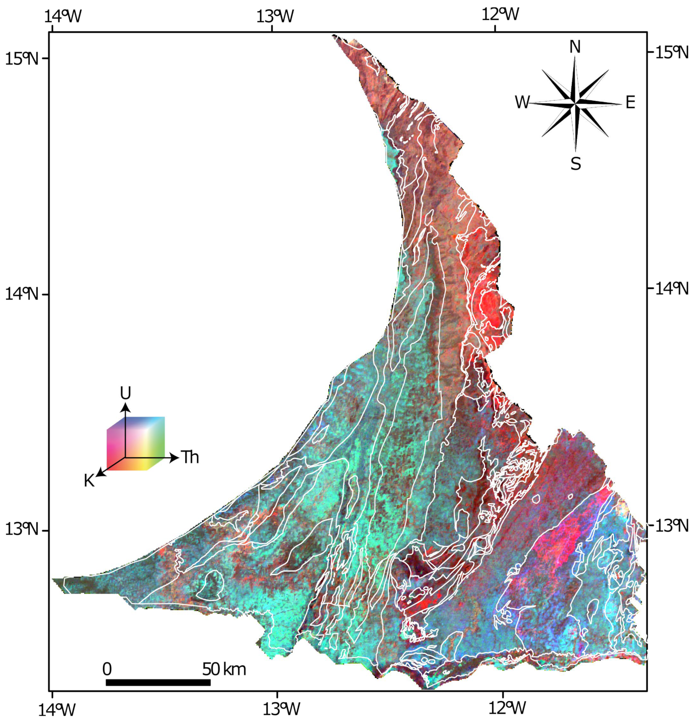
3.1. Airborne Radiometric Data

The acquisition and processing of airborne radiometric data of eastern Senegal were carried out in 2007 by Fugro Air borne Survey (Pt) Limited in collaboration with the Ministry of Economy and Finance of Senegal. Gamma ray measurements were performed using two Exploranium GPX-1024 (cubic inches) 256 (channels) spectrometers controlled by a GR820 console linked to the data acquisition system. A total area of 30,712 km2 was covered for a total flight distance of 133,817 km.
This total distance corresponds to several flight lines, oriented at 135 degrees N, with minimum lengths of 10,000 m. The spacing between two lines was of 250 m. The spacing was defined to highlight geological features or targets of economic interest. Data acquisition was performed every second at a flight altitude of 100 m, varying within 20 m. Flight velocity was about 67 m/s. After processing and interpolation on a regular grid, a map with a resolution of 62.5 m/pixel, giving information on the abundance of K, Th, and U, was generated. Note that the term “resolution” may be misleading in gamma ray investigations, since the value for a given pixel always includes contributions from sources outside that pixel [1]. The resulting radiometric map is shown in Figure 2 as a ternary representation, with K in the red channel, Th in the green channel, and U in the blue channel.

3.2. Topographic Information

The digital elevation model (DEM) used to calculate shaded relief and roughness maps (see Section 3.3 for roughness map calculation) was derived from the data of the Shuttle Radar Topography Mission (SRTM). SRTM data can be noisy, especially in relatively flat areas. Shared relief and roughness maps are sensitive to noisy data. The direct use of the 1”/pixel resolution SRTM data can lead to artefacts in roughness maps due to the various sources of noise in this data. The study [38] showed that the artefacts in roughness maps are essentially absent if the roughness calculation is applied to the 3”/pixel resolution de-noised SRTM data achieved by [39]. In these data, the absolute bias, strip noise, speckle noise, and tree height bias are separated and removed using multiple satellite data sets and filtering techniques. These improvements to the model have allowed for better vertical accuracy (±2 m), allowing a better representation of the topography of low relief areas. The shadow relief map is calculated with a sun elevation angle of 10° and an azimuth of 45°.

3.3. Roughness Calculation

Roughness is an intuitive concept that is vaguely defined as an estimate of the dispersion of elevations or slopes for a given baseline or length scale [40,41]. This technique has been used in Earth Science, with various applications reviewed by [41]. It has been even more widely used in Planetary Science where terrain is not generally accessible for in-situ investigations, except locally with landers and rovers [42,43,44,45,46,47]. There is not a unique mathematical definition of roughness. In this study, roughness was calculated following the approach of [48]. The roughness was calculated as the dispersion of detrended elevations (elevations after removal of the average plane) within a circular region. Roughness may be calculated for different length scales. The length scale or baseline of each roughness map is defined as the diameter of the circular region. The roughness value corresponds to the roughness of elevations within this circular region (cell) and is assigned to the center of the circle. These SRTM files produced by [39] are provided in cylindrical projection, with the cylindrical projection distances in pixels varying as a function of latitude. Elevations for points situated at a distance less than half of the baseline from the center of the cell are therefore extracted. Detrended elevations are then obtained by removing the average plane, determined by the least-squares method. The frequency distribution of these detrended elevations is then calculated. The roughness R, expressed in meters, is defined with the following formula (interquartile scale):
R = N 0.673 2 N 1 Q 3 Q 1
where N is the number of elevation points in the square region, and Q1 and Q3 are, respectively, the elevations of the first quartile (elevation value such that 25% of elevations are < Q1) and the third quartile (elevation value such as 75% of elevations > Q3). The normalization factor 0.673 is introduced so that R is equal to the standard deviation if the elevations follow a normal (Gaussian) distribution [48]. The choice of the minimum possible baseline is determined from the resolution of the topographic data, in order to have sufficient statistics for the roughness calculation (500 m baseline in our case). The maximum baseline has to be much lower than the dimension of the map so that the map has a sufficient number of pixels to provide significant spatial variations (10,000 m in our case). Then, it is also possible to achieve calculations for one or several intermediate length scales (2000 m here). The three roughness maps are then combined into a ternary RGB color representation with roughness at 500 m in the red channel, roughness at 2000 m in the green channel, and roughness at 10,000 m in the blue channel. With this representation, the black regions are smooth at all scales, and the white regions are rough at all scales. Regions appearing in red would be rough only at the short length scale, and regions appearing in blue would be rough only at the long length scale.

3.4. Calculation of the Statistical Parameters of K, Th, and U Concentration Distribution

The methodology consists of the calculation of the frequency distributions of K, Th, and U concentrations and their moments (mean, standard deviation, skewness, and kurtosis) within a sliding cell. The values calculated for each cell were assigned to the location of the center of each cell. The map was therefore dependent on two calculation parameters: the width of the sliding cell and the step between one cell and the next one (the resolution of the gridded data), which should be a fraction of the width of the sliding cell. The frequency distributions of K, Th, and U concentrations within a sliding cell were calculated with the kernel density estimation method (kde), a non-parametric method to estimate the probability density of a random variable. Thus, at the end of this calculation, we obtained a cube with 12 bands corresponding to the expected value, the variance (converted to its square root, the standard deviation), the skewness, and the kurtosis of the three radioelements. The width of the sliding cell was determined to be large enough in order to have enough statistics within a cell to calculate the frequency distributions of concentrations and small enough to produce a map with significant spatial variations (or total number of pixels). In our case, we chose a sliding cell of 51 pixels × 51 pixels (about 3 km in length). The step was chosen equal to 1/10th of the width of the slide cell (5 pixels), which therefore corresponds to a 10% overlap between a cell and the next one. The final map had a resolution of 300 m and had dimensions of 933 per 992 (925,536 pixels).

3.5. Classification

3.5.1. UMAP

In order to visualize and analyze our 12-dimension data product of the statistical parameters for K, Th, and U, we needed to reduce its dimension. There are a large number of dimension reduction techniques, which can be classified broadly into two categories, matrix factorization and neighbor graphs. The well-known PCA analysis (Principal Component Analysis) belongs to the first category, whereas the recent t-distributed Stochastic Neighbor Embedding (t-SNE) belongs to the second category [49]. The UMAP technique (UMAP standing for Uniform Manifold Approximation and Projection for Dimension Reduction) is a newer and faster non-linear dimension reduction approach that also best preserves the global structure in comparison with the t-SNE [50]. UMAP was therefore used as a first step to reduce the number of dimensions from 12 to 3. Then, the data were projected and visualized in this low-dimension space before applying the K-means clustering approach for classification.

3.5.2. K-Means Clustering

K-means clustering is one of the most popular unsupervised machine learning algorithms. It aims at partitioning, in k clusters, n data or observations according to their similarities. For a number of k clusters, the algorithm starts by selecting k centroids. Each observation is then assigned to the cluster whose centroid is closest.
K-means clustering minimizes within-cluster variances (squared Euclidean distances). The centroids are recalculated and repositioned so that the sum V of the within-cluster variances (squared Euclidean distances) is minimized as given by:
V = j = 1 k i = 1 n x i j C j 2
where k is the number of clusters and Cj is the centroid of the cluster j.
This method, however, only finds the optimal centroids for a given fixed number of clusters k and does not determine the optimal number of clusters k itself for the data. This parameter can be determined by the elbow method, which consists of plotting the value of V as a function of the number of clusters and choosing the position of the inflection point as the optimal number of clusters.

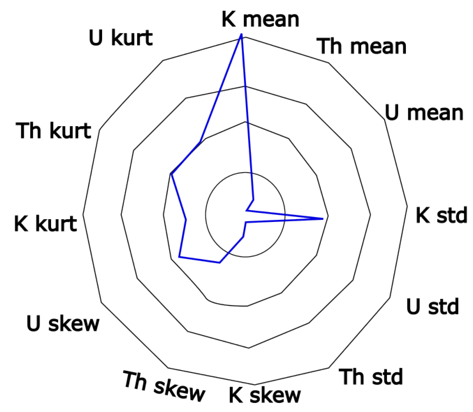
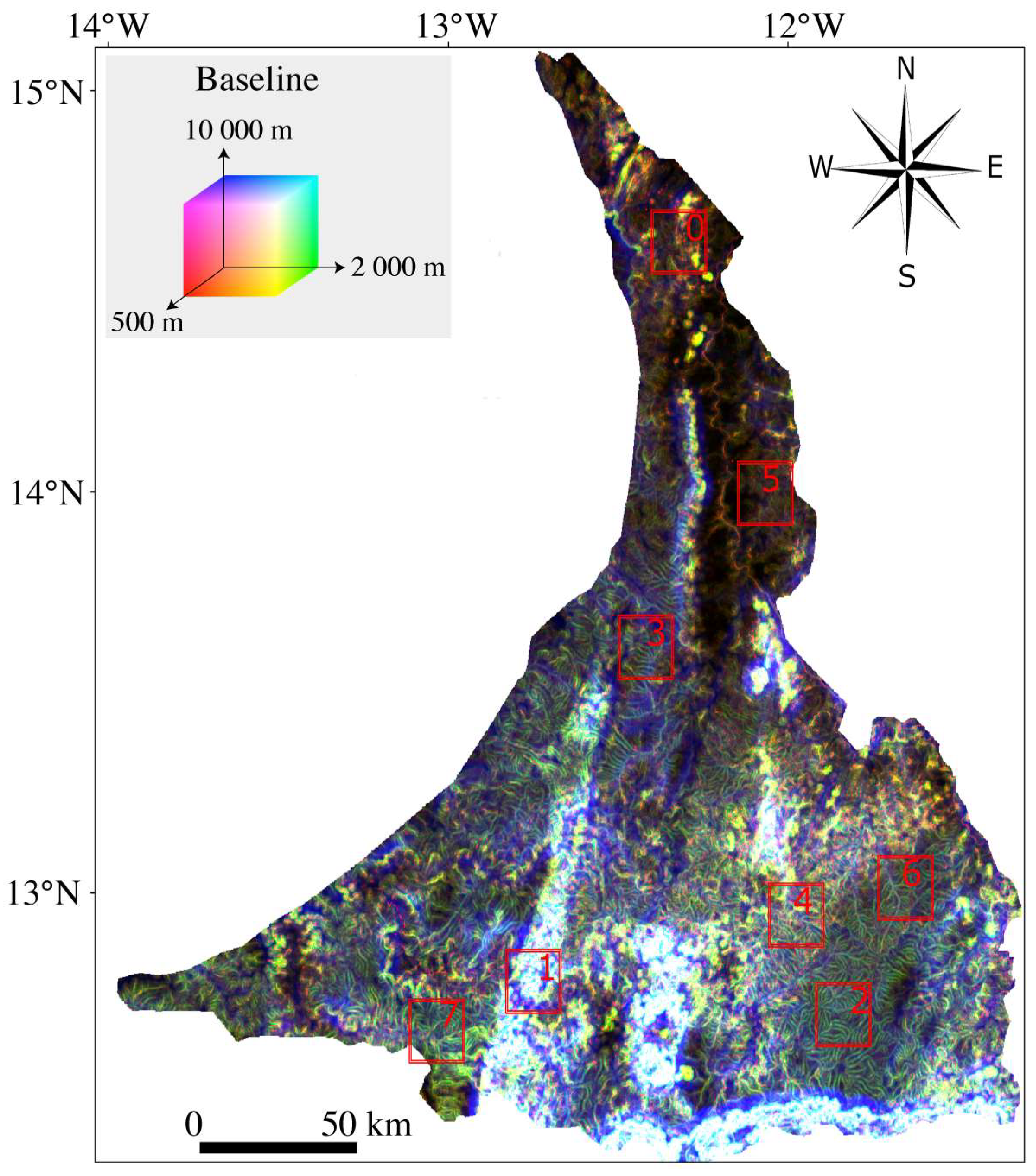
3.5.3. Plotting Statistical Signatures of Clusters with the Radar Plot

A radar plot was used to represent the statistical signature of each cluster obtained after the classification. It will be plotted here for each cluster after reducing and centering the set of statistical values. A radar graph, also called a spider graph, is a two-dimensional representation of several quantitative variables on an equi-angular radius starting from a single point. Each radius represents the value of one of the variables. The length of a radius is proportional to the magnitude of the variable relative to that of the other variables. In this study, the 12 variables are presented clockwise for K, Th, and U and the different moments, as illustrated in Figure 3. The label for each variation was then omitted in the final representation to make the figure less heavy. The signature of a unit was given by the shape of the polygon on the radargram. The statistical parameters need to be first centered and reduced.

4. Results

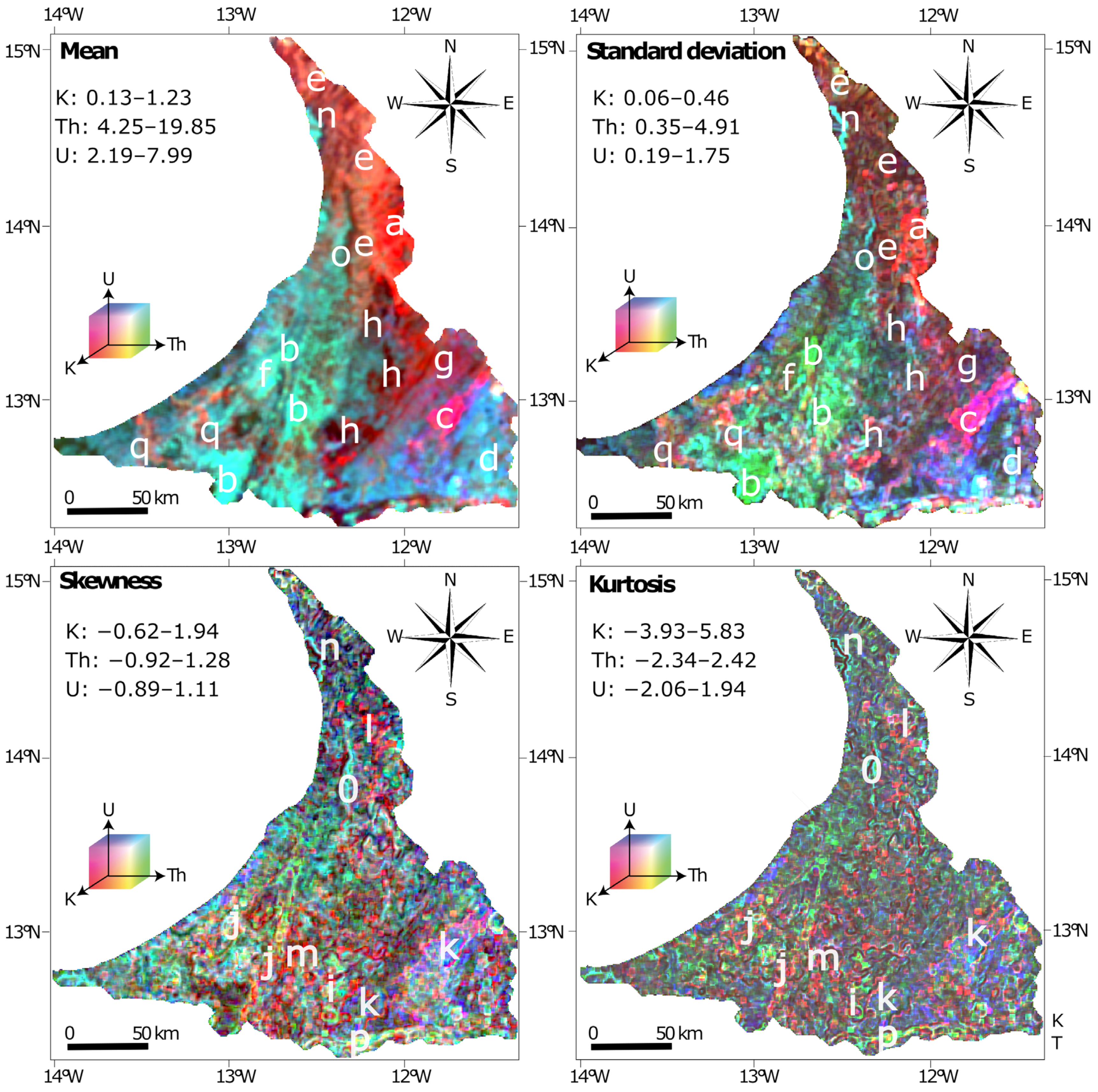
4.1. Maps of the Statistical Parameters of K, Th, and U Concentrations

The four statistical parameters (mean, standard deviation, skewness, and kurtosis) for each element are represented in Figure 4 in a ternary representation of K (red), Th (green), and U (blue). The map of means shows large units, with three main domains: a cyan domain in the west, enriched in Th and U; a red domain in the north and the central part, rich in K; and a pinkish and bluish domain towards the east richer in K and U. These domains are somewhat similar to those that can be visually defined from the standard deviation map, but with larger, more heterogeneous units on a shorter scale and sharp boundaries. We also note the existence of blue-green (cyan) curvilinear units in the northern part (label n, see next paragraph). The map of means and standard deviations are correlated in many places (cf. labels a, b, c, d, in Figure 4) but appear to be also not correlated and anti-correlated in others places (cf. labels e, f, g, h, in Figure 4).
The skewness map is clearly distinct from the mean and standard deviation maps. It is much more heterogeneous at short scales with large variations typically over a few kilometers, with many elongated features (lineaments), appearing in all kinds of hues in the ternary representation. Homogeneous regions of a significant extent (>10–20 km) with similar values of skewness are totally absent. The skewness is more often positive than negative (the distributions are more generally right-skewed). We report more frequent cyan colors (U and Th) towards the west, some yellowish-orange (cf. label i, j, Figure 4) and violet towards the east (cf. label k, Figure 4), and red (K) in the middle (cf. label l, m, Figure 4). The kurtosis map is similar to the skewness map and appears to provide limited additional information. It shows an even more heterogeneous signal with several elongated features (lineaments), often cyan (Th and U), red (K), or violet (K and U). The colors combining red and green hues (K and Th) faded in comparison to the skewness map. The curvilinear units in the northern part that are found in the standard deviation and skewness maps (cf. labels n and Figure 4) are also revealed in the kurtosis map. We also note a certain degree of correlation between the locations of units appearing in red and purple between the skewness map and the kurtosis map.

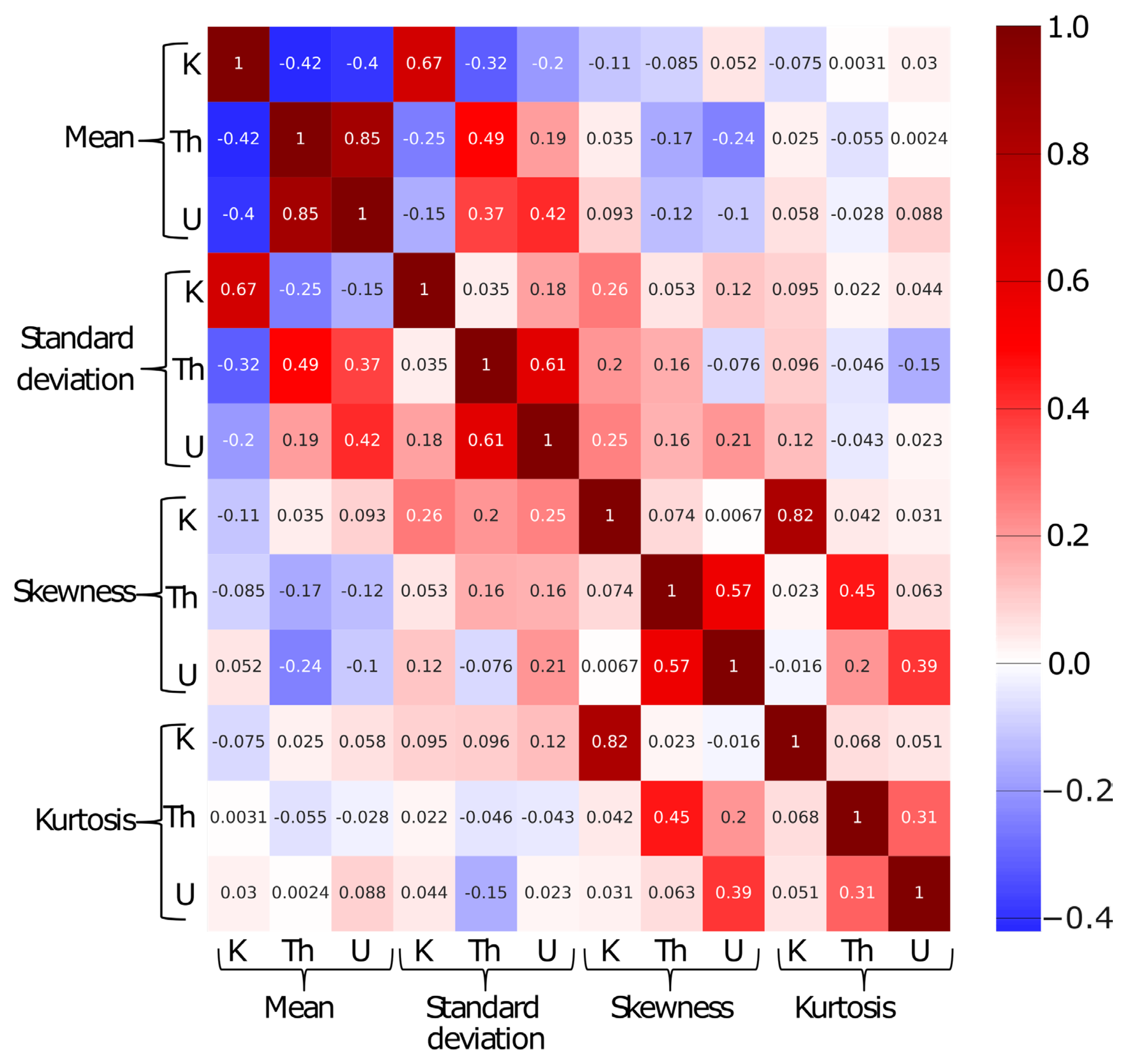
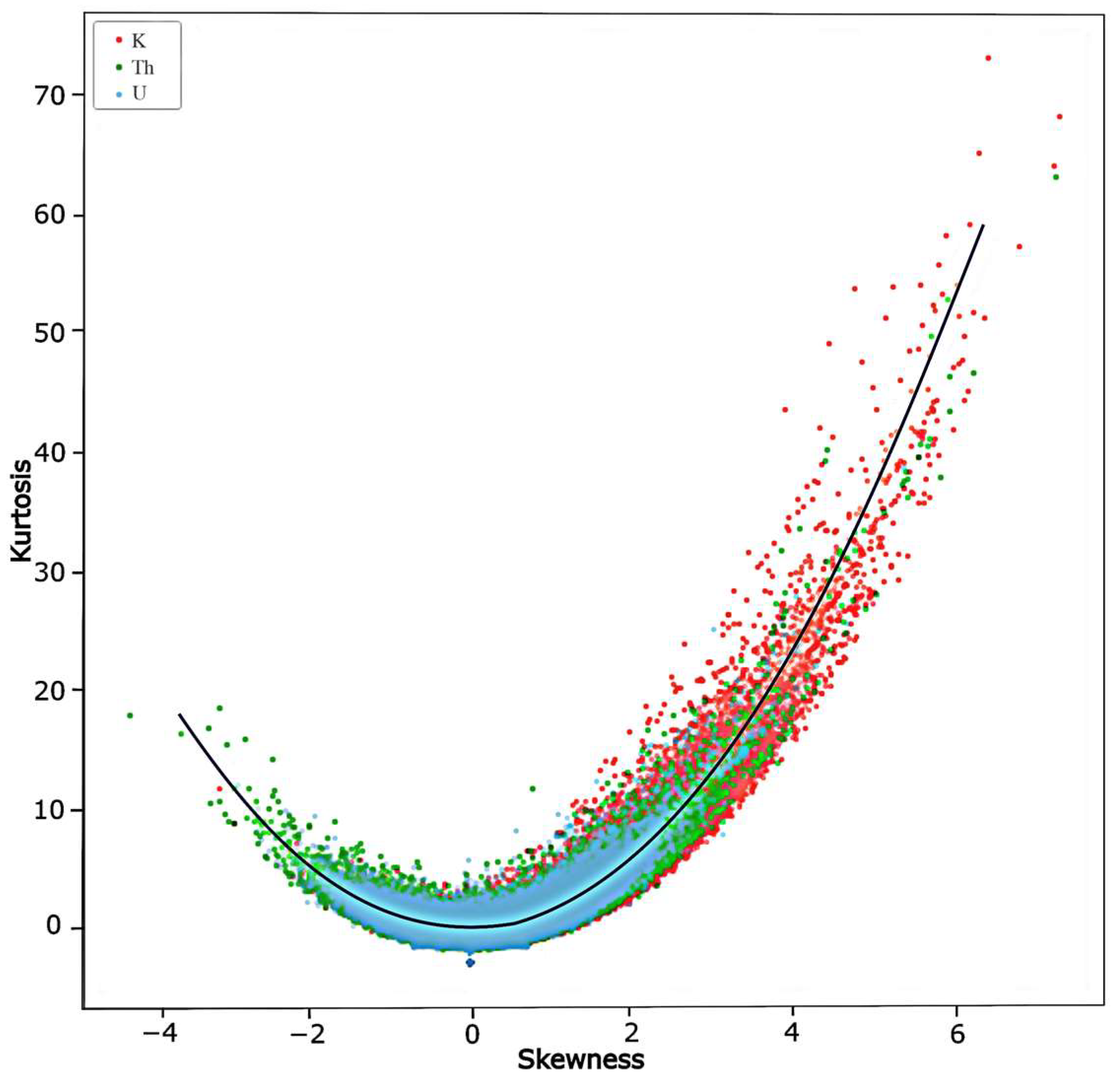
4.2. Correlation between the Statistical Parameters

To evaluate the correlation or absence of correlation between the different statistical parameters, we evaluated the correlation matrix (Figure 5). It confirmed the correlations between the means and standard deviations (0.67, 0.49, 0.42, for K, Th, and U, respectively). A strong correlation (0.85) was also reported between the mean values of Th and U. The correlation coefficient for the standard deviation and skewness of the two elements was also significantly high (0.61 and 0.57, respectively). Other notable correlations include the K skewness with the K kurtosis (0.82) and between the skewness and kurtosis for Th (0.45) and U (0.39). Anti-correlations are rare. Significant anti-correlations were only reported between the mean value of K and mean of Th (−0.42) and between the mean value of K and mean value of U (−0.40). Other combinations of parameters/elements did not show significant correlations or anti-correlations (correlation coefficient < 0.04 in absolute value).

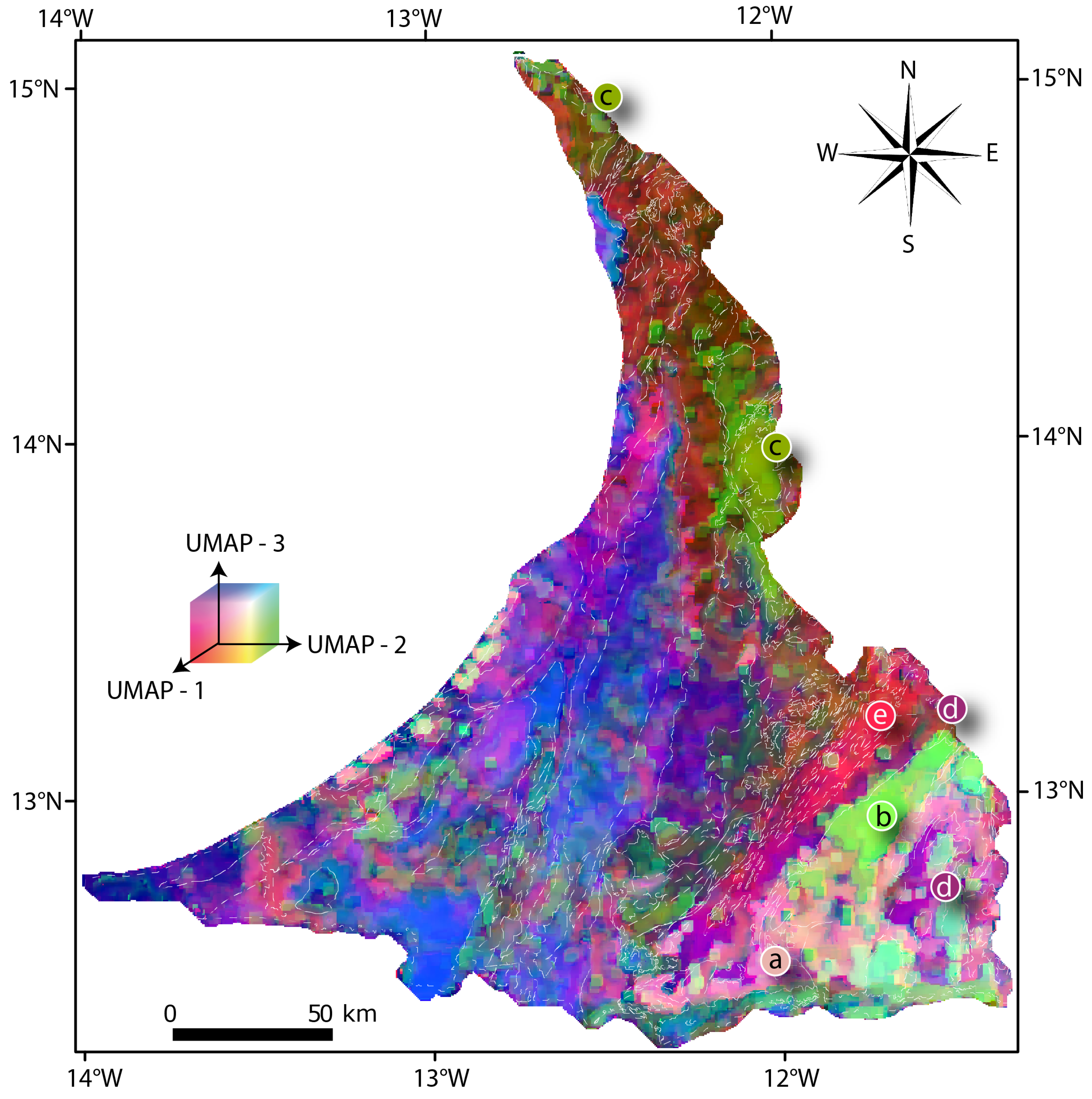
4.3. Statistical Map Visualization after Dimensionality Reduction

UMAP was used to reduce the twelve dimensions corresponding to the four statistical parameters for three elements to three dimensions while allowing the concentration of the maximum amount of information contained in these three parameters. The use of an algorithm to reduce the number of dimensions of the data product was justified by the existence of significant degrees of correlation between the different statistical parameters, as shown in the previous section. The visualization of the three new dimensions generated by UMAP is shown in Figure 6.
Comparing this result (Figure 6) with the radiometric map (Figure 2), we noticed that mapping based on statistical parameters offers different perspectives with new features that were not revealed on the standard ternary K, Th, and U representations. The combination of the 12 statistical parameters followed by a reduction of the dimension to three offers added values in comparison to the maps of statistical parameters, taken separately. For instance, the pinkish unit (label a, on Figure 6) had a unique signature in terms of statistical parameters and occurred on a specific location in the southeastern part of the map (the pinkish hue is not represented elsewhere on the map). The light green hue (label b, on Figure 6) also formed a well-defined unit and was also represented in the south as more or less isolated areas. The unit c (Figure 6), distinguished on the ternary map by a higher K concentration, is highlighted here by its unique statistical properties that spatially appear in two distinct areas. Finally, it seems to be possible to define visually two other units, labelled d and e on Figure 6, which was also suggested from Figure 2 (ternary representation), but the boundaries are sharper here and the differences in hues more apparent. These are only a few examples of units that can be defined—among others—from the visual examination of the map. A more quantitative assessment of the value of the statistical map is obtained in the next section by application of the clustering method.

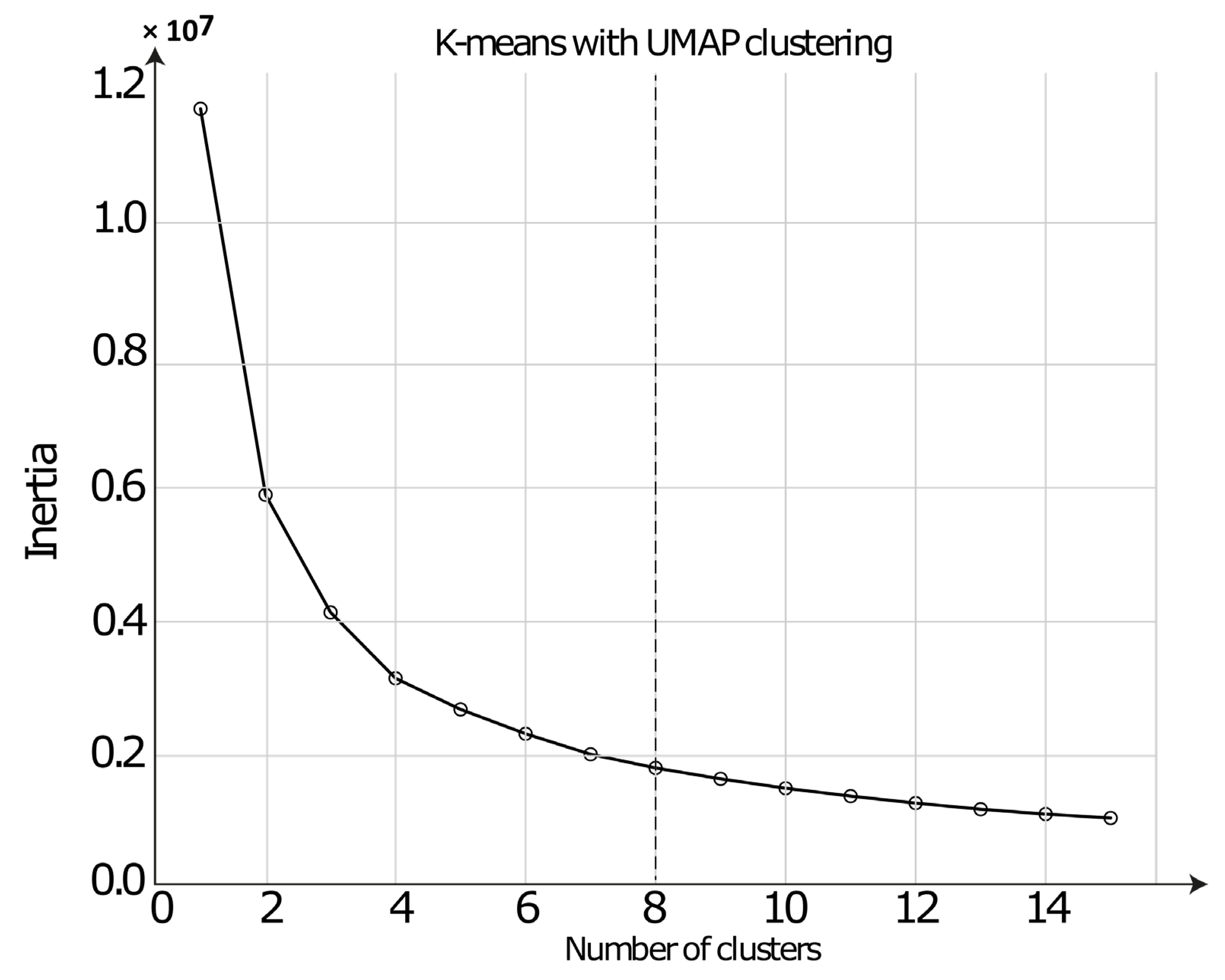
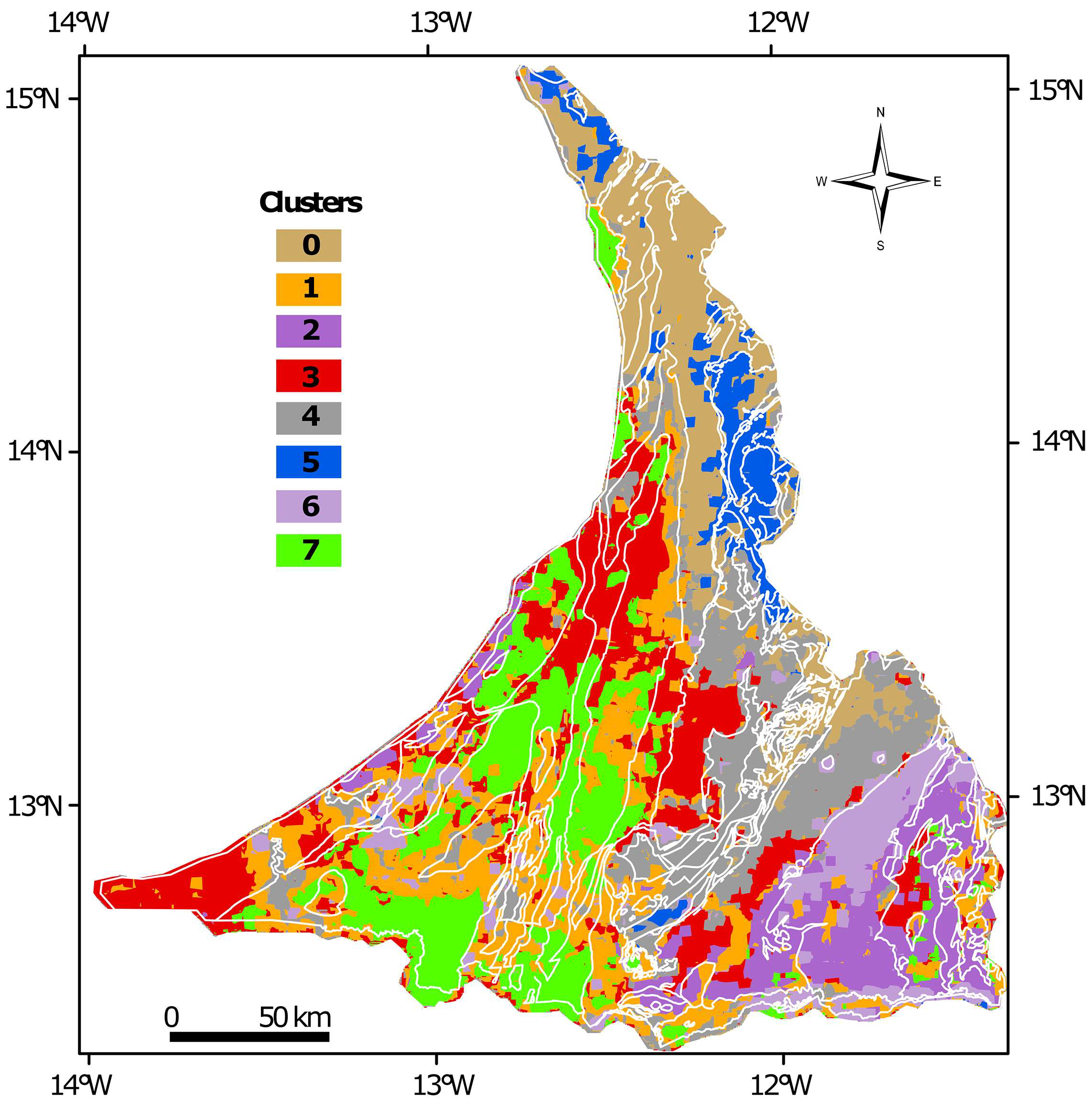
4.4. Clustering and Clusters Characteristic

The elbow method was used to find the optimal number k of clusters (Figure 7) to train the k-means clustering model on our data. It suggests a four to eight cluster segmentation. Based on the number of visually distinct hues in Figure 6, we selected the maximum number of clusters (eight) suggested by the elbow method. This number is justified by the natural complexity of the area, which would be likely “oversimplified” if reduced to only four clusters. The clusters were then plotted as a function of the statistical parameters on a box-plot (Figure 8) and we confirmed, as anticipated from the comparison of individual statistical maps, that the kurtosis parameter is not very discriminating.
The clusters formed large domains that are spatially continuous. A given cluster may appear as one large continuous domain or form more patchy units and occur as several smaller domains (Figure 9). However, they never appear as a large number of isolated areas (even if some statistical parameters vary over short distances). This suggests that these clusters have a physical meaning (hopefully in terms of geology or alteration processes, see discussion). The northern part was mapped with clusters 0 and 5 characterized by high K and low Th and U. Cluster 0 contained less scattered distributions, tending towards normal distributions with a skewness closer to 0, while cluster 5 had a larger standard deviation and right-skewed distributions (positive skewness). Clusters 1, 7, and 3 occurred on the western part. They are distinguished by their Th and U concentration distributions. Cluster 3 was much more enriched in Th (18 ppm) and U (6.6 ppm) than clusters 7 and 1 and had symmetrical Th distributions with elevated standard deviations and slightly left-skewed U distributions. Cluster 7 and 1 had similar U and Th contents but differed in that Th and U distributions were more scattered in cluster 1 and more symmetrical in cluster 7. In the center, we noted the occurrence of cluster 4, which contained the lowest contents of K, Th, and U. Clusters 2 and 6 occurred on the south eastern part and contained relatively high levels of Th and U, with cluster 6 enriched in K in the north. The Th and U distributions in the two clusters were equivalent, while the K distributions were more dispersed and asymmetrical (spread to the right) in cluster 6 than in cluster 2.

5. Discussion

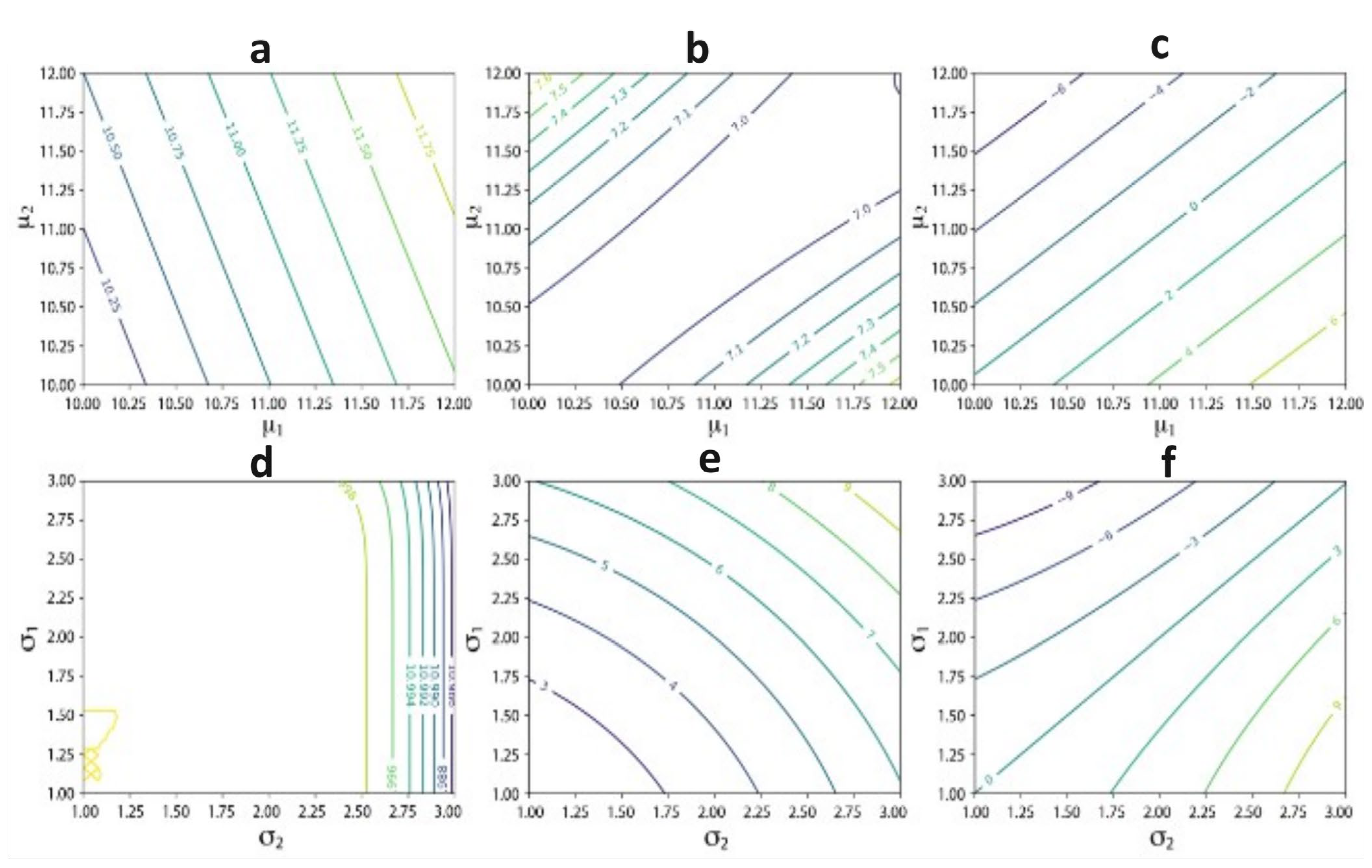
5.1. Interpretations of the Scales of Variations of the Statistical Parameters

It was noted that the skewness and kurtosis varied over a much shorter length-scale than the mean or standard deviation values. The same behavior was observed for the three elements. This means that, for overt short distances (typically <10 km), the mean values and standard deviation values of the concentrations vary more smoothly than the shape parameters (skewness and kurtosis) of their distributions. Since this effect was observed for the three elements, we postulated that this should be related to their common geochemical behavior with respect to magmatic processes (i.e., the fact that these elements are incompatible). Even in the presence of non-magmatic rocks, it is possible to assume that this general behavior is inherited from magmatic processes in the protolith. Within a homogeneous lithological domain, the shape of geochemical distributions may be relatively simple (multi-fractal, normal, or log-normal) [23]. However, depending of the scale of analysis, the distributions may be, in some cases, more complex. For instance, for an area comprising lithological contacts with rocks characterized by very different statistical parameters for K, Th, and/or U concentrations, this may result in more complex distributions than the multi-fractal, normal, or log-normal. We hypothesized that the spatial mixtures of “simple” distributions with different parameters lead to much higher variabilities (in a relative sense) in the higher-order moments than in the lower order moments. We are not aware of a theorem that can be invoked to confirm this hypothesis, but it may be easily verified by the numerical simulation of mixtures of distributions. In these simulations, we calculated the statistical parameters of the variable that would result from the mixture of two distributions with different means and different standard deviations. The results (Figure 10) illustrate the situations for the sum of two normal distributions with fixed means and variable standard deviations and those for the sum of two normal distributions with fixed standard deviations and variable means. Figure 10 confirms that the values of higher order moments vary over a larger range of values in comparison with lower order moment as a result of the mixture process. We proposed that the observed behavior, i.e., the shorter length-scale of variations of higher order moments, reflects the fact that some of the distributions, especially across the boundary of homogeneous lithological units, used to calculate the map of statistical parameters result from the mixture of normal/log-normal distributions. This hypothesis may only be tested by studies on geophysical surveys at a higher spatial resolution.

5.2. Interpretations of Correlations between Statistical Parameters

The different correlations and anti-correlations between the statistical parameters observed here can be interpreted on the basis of the studies of [23], who described the distributions of chemical elements and associated them with different geochemical processes, leading to the depletion or enrichment of these elements. The correlation between the observed means and standard deviations for K, Th, and U could be explained by the fact that the fractionation via magmatic processes of a crustal segment originally rich in K (high mean) will tend to produce more extreme variations (higher standard deviations) than another crustal segment of a lower mean concentration subjected to the same magmatic history.
The correlation between the statistical parameters of Th and U (mean and standard deviations) reflects their similar behavior during magmatic processes, and their anti-correlation with K parameters may reflect the importance of surface processes, which is responsible for the mobility of K, whereas Th and often U remain immobile.
Skewness and kurtosis are correlated for all elements, and this correlation is much more accentuated for K (0.82). In log-normal distributions, the skewness and kurtosis are directly related and can both be expressed as a function of the parameter σ of the distribution:
S k e w n e s s = e σ 2 + 2 e σ 2 1
and
k u r t o s i s = e 4 σ 2 + 2 e 3 σ 2 + 3 e 2 σ 2 6 ,
Figure 11 is a scatter plot presenting the relationships between skewness and kurtosis for each point of the statistical map, with the theoretical relationships between the skewness and kurtosis for log-normal distributions. The fact that the points are scattered along the theoretical curve relating the skewness and kurtosis implies that distributions with log-normal affinities were frequent in our analysis, confirming here the statement made by [23].

5.3. Relations between Clusters and Geological Units, Topography, and Roughness

The main question that is addressed in this section is also the most important one for geologists: what is the physical meaning of the units (clusters) that we produce with our statistical approach? Does it have a geological meaning? Do the clusters reflect alteration process? Do they provide any hints for mineral exploration? We must admit that the classification map based on the parameters of the K, Th, and U concentration distributions did not systematically correlate at first glance with the geological units in the region (Figure 12). However, some of the clusters can be correlated with roughness and topography. This confirms the influence of surface processes on the distribution of radioelements in eastern Senegal, but our classification is not totally independent of the underlying geology. In this complex signal, it is possible to recognize that cluster 4 corresponds to crystalline rocks with mafic affinities, and there is, therefore, little enrichment in K, Th, and U, whereas clusters 2, 5, and 6 are associated with felsic rocks. The K-rich cluster 5 corresponds to a biotite granite, and clusters 2 and 6 cover the Saraya granite in the southeast. Clusters 2 and 6 contain relatively high levels of Th and U, with cluster 6 enriched in K in the north. The Th and U distributions in both clusters are equivalent while the K distributions are more dispersed and skewed to the right in cluster 6 than in cluster 2. On the roughness map (Figure 13), cluster 6 shows a more developed small scale roughness than in cluster 2. These differences could be explained by the presence of transition between an erosional zone north of the granite (cluster 6) and a depositional zone south of the granite (cluster 2).
Cluster 6, which covers the northern part (erosion zone) of the Saraya granite, extends slightly to the south. It is interesting to note that cluster 6 shows a better correlation with the granitoid than map K (where it is easy to recognize the northern part of the Saraya granite). This demonstrates that the statistical approach was able to recognize the southern part of the Saraya Granite, which is less exposed, more altered, and impossible to recognize based on concentrations alone [26].
To the north, cluster 0 covers low-altitude and low-roughness areas (Figure 13). Rich in K with symmetrical distributions, it contains mainly detrital rocks and metasediments. This could be associated with a depositional zone of initially K-rich formations. In contrast, cluster 5 concerns the higher and rougher areas, also rich in K but showing asymmetrical distributions inclined to the right, which could suggest the presence of an erosion zone. This cluster comprises crystalline rocks and a small portion of metasediments.
The western part, rich in Th and U, is covered by clusters 1, 3, and 7 with different degrees of roughness. They contain detrital and metamorphic rocks.
Cluster 1 encompasses the roughest areas (white areas on the roughness map, Figure 13). The distributions associated with the cluster are significantly right-skewed and could be associated with erosion zones. It forms ridges in some places.
The physical meaning attributed to each of the clusters is summarized in Table 1. The statistical signature is represented by a radar plot, with statistical parameters ordered from lower moments to higher moments (mean, standard deviation, skewness, and kurtosis, see method section). This illustrates that each of our clusters is characterized by a unique shape on this radar plots. Further work in different areas could reveal if the observed signatures and their interpretation, which is generally defined as a lithology and an erosional context (active erosion versus lateritization or sedimentation) may be, at least partially, extended.

6. Conclusions

The aim of this study was to examine first the diversity of statistical parameters of K, Th, and U concentrations in Eastern Senegal as a case study to evaluate the potential value of advanced statistical analyses of airborne radiometric maps for geological mapping or for regolith mapping. For this purpose, we calculated maps of the local mean, standard deviation, skewness, and kurtosis of K, Th, and U concentrations, with a scale of 51 pixels × 51 pixels (about 3 km in length). We confronted these results to available geological information, topography, and roughness. We also produced a classification (clusters) based on the statistical values and attempted to interpret the clusters in terms of lithology and superficial processes. The examination of the maps of the statistical parameters revealed three principal results: (1) the mean and standard deviation values are generally correlated; (2) the typical length-scale of variations of statistical parameters is shorter for the mean and standard deviation than for the skewness and kurtosis; (3) the skewness and kurtosis are well correlated, and the kurtosis adds little information. The later result was predicted if distributions at the scale of analysis are close to log-normal distributions (a relationship exists between skewness and kurtosis for log-normal distribution). The scatter of points along this theoretical curve suggests that the distribution of the scale of analysis often corresponds to a log-normal distribution or a mixture of log-normal distributions. In addition, the mixture of log-normal distributions explains the result mentioned above (2) on the length scale of variations of statistical parameters.
The eight clusters or units obtained from statistical parameters do not show obvious correlations with geological units. However, we attempted to interpret them in terms of lithology plus an erosion context (areas of deposition/sedimentation, alteration, or regolith formation). Further studies may focus on the possible generalization of some of the statistical signatures observed in different parts of the world. It would be also interesting to apply this approach to high-resolution surveys, such as those generally achieved during the mineral exploration of exploration permits by the mining industry.

Author Contributions

Conceptualization: A.T., D.B., M.F. and G.F. Software: A.T. and D.B; formal analysis: A.T., D.B., M.F., G.F. and G.O. Data curation: A.T. and M.F.; writing—original draft: A.T., D.B., M.F., G.F. and G.O. writing review and editing: A.T., D.B., M.F. and G.F. All authors have read and agreed to the published version of the manuscript.

Funding

CEA-MEM, AGATE project, LMI MINERWA, grant number: 2122_SSCH_0010.

Data Availability Statement

The airborne radiometric data of Senegal can be obtained from the Direction de la Géologie du Sénégal.

Acknowledgments

Aïssata Thiam PhD fellowship was funded by the African Center of Excellence in Mining and Mining Environment (CEA-MEM, https://cea-mem.inphb.ci/, accessed on 23 March 2023) of the Houphouët Boigny National Polytechnic Institute, and she was supported by the French National Research Institute for Sustainable Development in the framework of the Joint International Laboratory for Responsible Mining in Africa (https://miner-wa.org, accessed on 23 March 2023). This research was also financially supported by the AGATE project (https://agate-project.org/, accessed on 23 March 2023).

Conflicts of Interest

The authors declare no conflict of interest.

References

  1. Dentith, M.; Mudge, S.T. Geophysics for the Mineral Exploration Geoscientist; Cambridge University Press: Cambridge, UK, 2014; ISBN 978-0-521-80951-1. [Google Scholar]
  2. Essa, K.S.; Munschy, M.; Youssef, M.A.S.; Khalaf, E.E.D.A.H. Aeromagnetic and Radiometric Data Interpretation to Delineate the Structural Elements and Probable Precambrian Mineralization Zones: A Case Study, Egypt. Min. Metall. Explor. 2022, 39, 2461–2475. [Google Scholar] [CrossRef]
  3. Eppelbaum, L.V.; Mishne, A.R. Unmanned Airborne Magnetic and VLF investigations: Effective Geophysical Methodology of the Near Future. Positioning 2011, 2, 112–133. [Google Scholar] [CrossRef]
  4. Amestoy, J.; Meslin, P.-Y.; Richon, P.; Delpuech, A.; Derrien, S.; Raynal, H.; Pique, É.; Baratoux, D.; Chotard, P.; Van Beek, P.; et al. Effects of environmental factors on the monitoring of environmental radioactivity by airborne gamma-ray spectrometry. J. Environ. Radioact. 2021, 237, 106695. [Google Scholar] [CrossRef] [PubMed]
  5. Minty, B.R.S. Fundamentals of airborne gamma-ray spectrometry. AGSO J. Aust. Geol. Geophys. 1997, 17, 39–50. [Google Scholar]
  6. Minty, B.R.S.; Luyendyk, A.P.J.; Brodie, R.C. Calibration and data processing for airborne gamma-ray spectrometry. AGSO J. Aust. Geol. Geophys. 1997, 17, 51–62. [Google Scholar]
  7. Berning, J. The Rossing uranium deposit. In Mineral Deposits of South Africa; Anhaeusser, C.R., Maske, S., Eds.; Geological Society of South Africa: Johannesburg, South Africa, 1986; pp. 1819–1832. [Google Scholar]
  8. Smith, R.J. Geophysics in Australian mineral exploration. Geophysics 1985, 50, 2637–2665. [Google Scholar] [CrossRef]
  9. Forman, J.M.A.; Angeiras, A.G. Poços de Calderas and Itataia: Two Case Histories of Uranium Exploration in Brazil; International Atomic Energy Agency: Vienna, Austria, 1981; pp. 99–139. [Google Scholar]
  10. Dentith, M.C.; Frankcombe, K.F.; Trench, A. Geophysical signatures of Western Australia mineral deposits: An overview. In Geophysical Signatures of Western Australian Mineral Deposits; Dentith, M.C., Frankcombe, K.F., Ho, S.E., Shepherd, J.M., Groves, D.I., Trench, A., Eds.; Publication 26, and Australian Society of Exploration Geophysicists, Special Publication; The University of Western Australia: Crawley, Australia, 1994; Volume 7, pp. 29–84. [Google Scholar]
  11. Bucher, B.; Rybach, L.; Schwarz, G. Search for long-term radiation trends in the environs of Swiss nuclear power plants. J. Environ. Radioact. 2008, 99, 1311–1318. [Google Scholar] [CrossRef]
  12. Paridaens, J. Development of a low cost, GPS-based upgrade to a standard handheld gamma detector for mapping environmental radioactive contamination. Appl. Radiat. Isot. 2006, 64, 264–271. [Google Scholar] [CrossRef]
  13. Rybach, L.; Bucher, B.; Schwarz, G. Airborne surveys of Swiss nuclear facility sites. J. Environ. Radioact. 2001, 53, 291–300. [Google Scholar] [CrossRef]
  14. Sanderson, D.C.W.; Cresswell, A.J.; Hardeman, F.; Debauche, A. An airborne gamma-ray spectrometry survey of nuclear sites in Belgium. J. Environ. Radioact. 2004, 72, 213–224. [Google Scholar] [CrossRef]
  15. Elkhateeb, S.O.; Abdellatif, M.A.G. Delineation potential gold mineralization zones in a part of Central Eastern Desert, Egypt using Airborne Magnetic and Radiometric data. NRIAG J. Astron. Geophys. 2018, 7, 361–376. [Google Scholar] [CrossRef]
  16. Metelka, V.; Baratoux, L.; Naba, S.; Jessell, M.W. A geophysically constrained litho-structural analysis of the Eburnean greenstone belts and associated granitoid domains, Burkina Faso, West Africa. Precambrian Res. 2011, 190, 48–69. [Google Scholar] [CrossRef]
  17. Morris, P.A.; Pirajno, F.; Shevchenko, S. Proterozoic mineralization identified by integrated regional regolith geochemistry, geophysics and bedrock mapping in Western Australia. Geochem. Explor. Environ. Anal. 2003, 3, 13–28. [Google Scholar] [CrossRef]
  18. Scott, K.M.; Pain, C. Regolith Science; Springer: Dordrecht, The Netherlands, 2008; ISBN 978-1-4020-8859-9. [Google Scholar]
  19. Metelka, V.; Baratoux, L.; Jessell, M.W.; Barth, A.; Ježek, J.; Naba, S. Automated regolith landform mapping using airborne geophysics and remote sensing data, Burkina Faso, West Africa. Remote Sens. Environ. 2018, 204, 964–978. [Google Scholar] [CrossRef]
  20. Dickson, B.; Scott, K. Interpretation of aerial gamma-ray surveys—Adding the geochemical factors. AGSO J. Aust. Geol. Geophys. 1997, 17, 187–199. [Google Scholar]
  21. Ahrens, L.H. The lognormal distribution of the elements (A fundamental law of geochemistry and its subsidiary). Geochim. Cosmochim. Acta 1954, 5, 49–73. [Google Scholar] [CrossRef]
  22. Wijs, H.J. Statistics of ore distribution: (2) Theory of binomial distribution applied to sampling and engineering problems. Geol. Mijnb. 1953, 15, 12–24. [Google Scholar]
  23. Allegre, C.J.; Lewin, E. Scaling laws and geochemical distributions. Earth Planet. Sci. Lett. 1995, 132, 1–13. [Google Scholar] [CrossRef]
  24. Turcotte, D.L. A fractal approach to the relationship between ore grade and tonnage. Econ. Geol. 1986, 81, 1528–1532. [Google Scholar] [CrossRef]
  25. Fall, M.; Baratoux, D.; Ndiaye, P.M.; Jessell, M.; Baratoux, L. Multi-scale distribution of Potassium. Thorium and Uranium in Paleoproterozoic granites from eastern Senegal. J. Afr. Earth Sci. 2018, 148, 30–51. [Google Scholar] [CrossRef]
  26. Fall, M.; Baratoux, D.; Jessell, M.; Ndiaye, P.M.; Vanderhaeghe, O.; Moyen, J.F.; Baratoux, L.; Bonzi, W.M.-E. The redistribution of thorium, uranium, potassium by magmatic and hydrothermal processes versus surface processes in the Saraya Batholith (Eastern Senegal): Insights from airborne radiometrics data and topographic roughness. J. Geochem. Explor. 2020, 219, 106633. [Google Scholar] [CrossRef]
  27. Moyen, J.-F.; Cuney, M.; Baratoux, D.; Sardini, P.; Carrouée, S. Multi-scale spatial distribution of K, Th and U in an Archaean potassic granite: A case study from the Heerenveen batholith, Barberton Granite-Greenstone Terrain, South Africa. S. Afr. J. Geol. 2021, 124, 53–86. [Google Scholar] [CrossRef]
  28. Baratoux, D.; Fall, M.; Meslin, P.-Y.; Jessell, M.W.; Vanderhaeghe, O.; Moyen, J.-F.; Ndiaye, P.M.; Boamah, K.; Baratoux, L.; André-Mayer, A.-S. The Impact of Measurement Scale on the Univariate Statistics of K, Th, and U in the Earth Crust. Earth Space Sci. 2021, 8, e2021EA001786. [Google Scholar] [CrossRef]
  29. Abouchami, W.; Boher, M.; Michard, A.; Albarede, F. A major 2.1 Ga event of mafic magmatism in west Africa: An Early stage of crustal accretion. J. Geophys. Res. 1990, 95, 17605. [Google Scholar] [CrossRef]
  30. Boher, M.; Abouchami, W.; Michard, A.; Albarede, F.; Arndt, N.T. Crustal growth in West Africa at 2.1 Ga. J. Geophys. Res. 1992, 97, 345. [Google Scholar] [CrossRef]
  31. Lemoine, S.; Tempier, P.; Bassot, J.P.; Caen-Vachette, M.; Vialette, Y.; Wenmenga, U.; Touré, S. The Burkinian, an orogenic cycle, precursor of the Eburnean of West Africa. Coll. Afr. Geol. 13th 1985, 27. [Google Scholar]
  32. Bassot, J.P.; Bonhomme, M.; Roques, M.; Vachette, M. Mesures d’âges absolus sur les séries précambriennes et paléozoïques du Sénégal oriental. Bull. Société Géologique Fr. 1963, S7-V, 401–405. [Google Scholar] [CrossRef]
  33. Bassot, J.P.; Caen-Vachette, M. Données géochronologiques et géochimiques nouvelles sur les granitoïdes de l’est Sénégal: Implications sur l’histoire géologique du birimien de cette région. In Géologie Africaine; Klerkx, J., Michot, J., Eds.; Musée Royal de l’Afrique Centrale: Tervuren, Belgium, 1983. [Google Scholar]
  34. Feybesse, J.L.; Milési, J.P.; Johan, Y.; Dommanget, A.; Calvez, J.-Y.; Boher, M.; Abauchami, W. La limite Archéen-Protérozoïque d’Afrique de l’Ouest: Une zone de chevauchement antérieure à l’accident de Sanssandra, l’exemple de la région de d’Odienne et de Touba (Cote d’Ivoire). C.R. Acad. Sci. Paris 1989, 309, 1847–1853. [Google Scholar]
  35. Liégeois, J.P.; Claessens, W.; Camara, D.; Klerkx, J. Short-lived Eburnian orogeny in southern Mali. Geology, tectonics, U-Pb and Rb-Sr geochronology. Precambrian Res. 1991, 50, 111–136. [Google Scholar] [CrossRef]
  36. Bassot, J.P. Le complexe volcano-plutonique calco-alcali de la rivière daléma (Est Sénégal): Discussion de sa signification géodynamique dans le cadre de l’orogénie eburnéenne (protérozoïque inférieur). J. Afr. Earth Sci. 1983 1987, 6, 505–519. [Google Scholar] [CrossRef]
  37. Milési, J.-P.; Ledru, P.; Feybesse, J.-L.; Dommanget, A.; Marcoux, E. Early proterozoic ore deposits and tectonics of the Birimian orogenic belt, West Africa. Precambrian Res. 1992, 58, 305–344. [Google Scholar] [CrossRef]
  38. Niang, I. Traitement de Données Topographiques srtm pour L’établissement d’une Carte de Rugosité sur l’Afrique de l’Ouest. Master’s Thesis, University Cheikh Anta Diop, Institut des Sciences de la Terre, Dakar, Senegal, 2018. [Google Scholar]
  39. Yamazaki, D.; Ikeshima, D.; Tawatari, R.; Yamaguchi, T.; O’Loughlin, F.; Neal, J.C.; Sampson, C.C.; Kanae, S.; Bates, P.D. A high-accuracy map of global terrain elevations: Accurate Global Terrain Elevation map. Geophys. Res. Lett. 2017, 44, 5844–5853. [Google Scholar] [CrossRef]
  40. Shepard, M.K.; Campbell, B.A.; Bulmer, M.H.; Farr, T.G.; Gaddis, L.R.; Plaut, J.J. The roughness of natural terrain: A planetary and remote sensing perspective. J. Geophys. Res. Planets 2001, 106, 32777–32795. [Google Scholar] [CrossRef]
  41. Smith, M.W. Roughness in the Earth Sciences. Earth-Sci. Rev. 2014, 136, 202–225. [Google Scholar] [CrossRef]
  42. Cord, A.; Baratoux, D.; Mangold, N.; Martin, P.; Pinet, P.; Greeley, R.; Costard, F.; Masson, P.; Foing, B.; Neukum, G. Surface roughness and geological mapping at subhectometer scale from the High Resolution Stereo Camera onboard Mars Express. Icarus 2007, 191, 38–51. [Google Scholar] [CrossRef]
  43. Kreslavsky, M.A.; Head, J.W. Kilometer-scale roughness of Mars: Results from MOLA data analysis. J. Geophys. Res. Planets 2000, 105, 26695–26711. [Google Scholar] [CrossRef]
  44. Kreslavsky, M.A.; Head, J.W.; Neumann, G.A.; Rosenburg, M.A.; Aharonson, O.; Smith, D.E.; Zuber, M.T. Lunar topographic roughness maps from Lunar Orbiter Laser Altimeter (LOLA) data: Scale dependence and correlation with geologic features and units. Icarus 2013, 226, 52–66. [Google Scholar] [CrossRef]
  45. Lemelin, M.; Daly, M.G.; Deliège, A. Analysis of the Topographic Roughness of the Moon Using the Wavelet Leaders Method and the Lunar Digital Elevation Model From the Lunar Orbiter Laser Altimeter and SELENE Terrain Camera. J. Geophys. Res. Planets 2020, 125, e2019JE006105. [Google Scholar] [CrossRef]
  46. Pommerol, A.; Chakraborty, S.; Thomas, N. Comparative study of the surface roughness of the Moon, Mars and Mercury. Planet. Space Sci. 2012, 73, 287–293. [Google Scholar] [CrossRef]
  47. Rosenburg, M.A.; Aharonson, O.; Head, J.W.; Kreslavsky, M.A.; Mazarico, E.; Neumann, G.A.; Smith, D.E.; Torrence, M.H.; Zuber, M.T. Global surface slopes and roughness of the Moon from the Lunar Orbiter Laser Altimeter. J. Geophys. Res. 2011, 116, E02001. [Google Scholar] [CrossRef]
  48. Aharonson, O.; Zuber, M.T.; Rothman, D.H. Statistics of Mars’ topography from the Mars Orbiter Laser Altimeter: Slopes, correlations, and physical Models. J. Geophys. Res. Planets 2001, 106, 23723–23735. [Google Scholar] [CrossRef]
  49. Van der Maaten, L.; Hinton, G. Viualizing data using t-SNE. J. Mach. Learn. Res. 2008, 9, 2579–2605. [Google Scholar]
  50. McInnes, L.; Healy, J.; Melville, J. UMAP: Uniform Manifold Approximation and Projection for Dimension Reduction. arXiv 2018, arXiv:1802.03426. [Google Scholar]
Figure 1. Simplified geological map of eastern Senegal based on the geological map of a 1:500,000 scale elaborated in the framework of the project 9 ACP SE 009 PASMI (2010). MTZ: Main Transcurrent Zone. The white labels from a to h correspond with the domains that are discussed in Section 4.1. The upper left insert represents the location of the region of study (KKI, standing for Kedougou-Kenieba Inlier).
Geosciences 13 00263 g001
Figure 2. Airborne radiometric data of eastern Senegal, 2007, overlayed with lithologic boundaries (see Figure 1 for the meaning of the geological units). K concentrations are indicated in the red channel (from 0 to 1.27 wt%), Th concentrations (from 0 to 19.35 ppm) in the green channel, and U concentrations (from 0 to 7.31 wt%) in the blue channel.
Geosciences 13 00263 g002
Figure 3. Example of a radar plot corresponding to the statistical signature of a cluster. Sdt = standard deviation.
Geosciences 13 00263 g003
Figure 4. Spatial repartition of the statistical parameters of the K, Th, and U content distributions. White labels from a to q correspond to areas discussed in the text.
Geosciences 13 00263 g004
Figure 5. Correlation matrix of statistical parameters of airborne K, Th, and U concentration distributions measured in Eastern Senegal.
Geosciences 13 00263 g005
Figure 6. Visualization of the radiometric data according to the three new dimensions generated from the reduction of the map of the distribution parameters of K, Th, and U with UMAP. Labels represent areas discussed in the text (the color under the letter represents the typical hue of the corresponding area).
Geosciences 13 00263 g006
Figure 7. Elbow method to determine the optimal number of clusters.
Geosciences 13 00263 g007
Figure 8. Variation of the mean, standard deviation, skewness, and kurtosis of the K, Th, and U distribution in each of the eight clusters delineated after the application of the K-means algorithm.
Geosciences 13 00263 g008
Figure 9. Segmented images according to statistical parameters (mean, standard deviation, skewness, kurtosis) of K, Th, and U content distributions. Number of clusters = 8. White labels (n and o) correspond to areas discussed in the text.
Geosciences 13 00263 g009
Figure 10. Illustration of the effects of the spatial mixing of normal distributions on the statistical parameters of mixed distributions. The graphs represent, from right to left, the mean (c,f), standard deviations (b,e), and skewness (a,d) of a variable assumed to be described by the mixture of two normal distributions. (ac): the two distributions have fixed standard deviations (σ1 = 1 and σ2 = 3) and variable means (m1 and m2, represented on the x and y-axes). (df): the two distributions have fixed means (m1 = 10 and m2 =12) and variable standard deviations s1 and s2, represented on the x and y-axes.
Geosciences 13 00263 g010
Figure 11. Relationship between skewness and kurtosis for different cases of processes leading to lognormal distributions. Red, green, and blue dots correspond to K, Th, and U statistical parameters, respectively.
Geosciences 13 00263 g011
Figure 12. Radiometric map classified according to statistical parameters of K, Th, and U concentration distributions overlaying geological boundaries of eastern Senegal.
Geosciences 13 00263 g012
Figure 13. Rough map, tricolor, baseline: 500 (red), 2000 (green), 10,000 (blue). The red squares represent the location of the roughness samples set for each cluster in Table 1. The numbers correspond to the clusters.
Geosciences 13 00263 g013
Table 1. Physical meaning of the different clusters. The radar plot presented in the statistical signature column was obtained from reduced and centered statistical parameters, ordered clockwise in the following way: mean values for K, Th, and U (upper right quadrant); standard deviations for K, Th, and U (lower right quadrant); skewness values for K, Th, and U (lower left quadrant); and kurtosis for K, Th, and U (upper left quadrant).
LithologyStatistical SignatureRoughnessPhysical Meaning
Cluster 0Metamorphic and detrital rocksGeosciences 13 00263 i001Geosciences 13 00263 i002
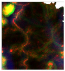
K-rich detrital formation deposit zone
Cluster 1Detrital, metamorphic and basic rocksGeosciences 13 00263 i003Geosciences 13 00263 i004
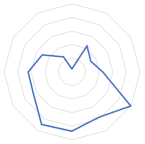
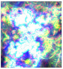
Active erosion area over various lithologies
Cluster 2Southern part of the Saraya graniteGeosciences 13 00263 i005Geosciences 13 00263 i006Sedimentation zone, lateritic surface on top of granitoid rocks
Cluster 3Detrital and metamorphic rocksGeosciences 13 00263 i007Geosciences 13 00263 i008Sedimentation area, lateritic surface on top of metamorphic rocks
Cluster 4Intermediate to mafic rocks, volcano-sedimentaryGeosciences 13 00263 i009Geosciences 13 00263 i010
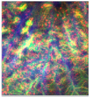
Follows drainage networks
Cluster 5Biotite granite, metasedimentsGeosciences 13 00263 i011Geosciences 13 00263 i012
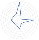
Active erosion area over granite and metasediments
Cluster 6Northern part of the Saraya graniteGeosciences 13 00263 i013Geosciences 13 00263 i014
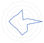
Active erosion area over granitoids rocks
Cluster 7Detrital rocks and carbonatesGeosciences 13 00263 i015Geosciences 13 00263 i016Sedimentation area, lateritic surface over clasts and carbonates
Disclaimer/Publisher’s Note: The statements, opinions and data contained in all publications are solely those of the individual author(s) and contributor(s) and not of MDPI and/or the editor(s). MDPI and/or the editor(s) disclaim responsibility for any injury to people or property resulting from any ideas, methods, instructions or products referred to in the content.

