Abstract
A spectral analysis of the time dynamics of seismicity occurring in the Enguri area of Georgia from 1978 to 2021 is performed by means of Schuster’s spectrum analysis, periodogram analysis, and empirical mode decomposition. The results of our analysis suggest that earthquakes around the reservoir (within a 50 km radius from the center of the dam) may be due to changes in water level, featured by the yearly cycle of loading and unloading operations of the reservoir. It is observed that the impacts of water fluctuations are more pronounced in shallower strata (down to 10 km) than deeper ones (down to 20 km); this could indicate that earthquakes occurring at deeper levels may primarily result from tectonic forces, whereas those at shallower depths may be predominantly triggered by reservoir-induced factors.
1. Introduction
Reservoir-triggered seismicity is investigated worldwide for its potential to cause damage to buildings, structures and, more critically, human lives. It initially came to attention in the Koyna region (India) following a significant earthquake with a magnitude of 6.3 in 1967, marking the most powerful event recorded in the area [1]. This occurrence became a focal point for extensive research [2,3,4,5]. Subsequently, Koyna has witnessed persistent triggered seismicity, notably linked to fluctuations in the water level of the dam [6]. Beyond Koyna, reservoir-triggered seismicity has been documented globally, including instances in the Nurek Reservoir, Tajikistan [7]; in the LG3 and Manic 3 reservoirs in Quebec, Canada [8]; and in the Govind Ballav Pant Reservoir in central India [9], among others.
Typically associated with additional static loading, such as the weight of the water reservoir and its seasonal variations, as well as factors like tectonic faults, liquefaction, and pore pressure variations, reservoir-triggered seismicity has been the subject of numerous investigations [10,11,12,13,14,15,16,17,18,19,20,21,22]. The consensus from these studies is that the filling of reservoirs has a discernible impact on the Earth’s crust, influencing the seismicity in areas already prone to earthquakes.
While distinguishing reservoir-triggered seismicity from naturally occurring tectonic seismicity remains a challenge, certain features are indicative of triggered earthquakes. These include a higher b value, a larger magnitude ratio of the largest aftershock to the mainshock, and an increase in seismicity rate corresponding to a rise in water level [23]. However, for a reliable assessment of the reservoir-triggered nature of seismicity, it is necessary to accurately identify and quantify the correlation with the reservoir water level, which serves as the driving force behind the temporal dynamics of the earthquake process.
Typically, the reservoir water level exhibits a recurring annual oscillatory pattern, implying that fluctuations in the water level should be mirrored in seismic activity. Consequently, it is essential to identify periodicities in the temporal distribution of seismicity that align with those observed in the variations of the water level. This step is crucial for assessing the dynamic link between the two processes—seismic and hydrologic.
In this study, we explore the time dynamics of local seismic activity in the vicinity of the Enguri hydro power station reservoir. Situated in western Georgia, this reservoir boasts the tallest arch dam in Europe. Drawing upon the initial assumptions regarding reservoir-triggered seismicity upon the initiation of large reservoir operations, our investigation is centered on examining the potential impact of the periodic variations in reservoir water level on the dynamic characteristics of local seismic activity.
The paper is organized as follows. In Section 2, the seismotectonic settings of the investigated area is presented. In Section 3, the seismic catalogue is described. Section 4 outlines the methods of analysis of earthquake data (the periodogram analysis, Schuster’s spectrum, and the empirical mode decomposition, which is employed to examine the temporal fluctuations in the monthly number of earthquakes by decomposing into a certain number of independent components). The results are presented in Section 5, and the conclusions are summarized in Section 6.
2. Seismo-Tectonic Settings
Georgia, situated within the Caucasus region, is positioned in the collision zone of the Eurasian and Afro-Arabian plates, forming part of the Mediterranean (Alpine–Himalayan) belt, at the interface of the European and Asian segments. Numerous publications provide comprehensive insights into the tectonics and geodynamics of Georgia, contributing to a thorough understanding of the region’s geological characteristics [24,25,26,27,28,29,30,31,32,33,34,35,36,37,38,39,40,41,42,43,44,45].
According to GPS data, the rate of this convergence is up to 30 mm/year [37,46,47,48]. The convergence rate across the Lesser Caucasus is up to 10 mm/year, while in the Greater Caucasus, it reaches values up to 4 mm/year [35,37,49]. The rate of convergence between the Lesser and Greater Caucasus increases from approximately 4 mm/year in the Rioni basin to about 14 mm/year in the Kura Basin [35,37,40,49,50,51,52,53,53]. The Enguri area, situated in western Georgia, is characterized by three main tectonic units, each with distinct geological development structures. A comprehensive description of these units is provided in a recent publication by Karamzadeh et al. [54]. The intricate network of faults mapped in Georgia relies predominantly on the displacement observed in key geological units. Additionally, certain faults have been tentatively categorized as potentially Quaternary in age, drawing insights from geological and tectonic maps, as well as the distribution of earthquake epicenters. Figure 1 illustrates two models of active faults, as developed by Caputo et al. [55], for the examined area. Notably, there are significant discrepancies between these two models. While the orientation of the active faults in the north in both models aligns with the general “Caucasian” trend, ranging from WNW/W to ESE/E, with a transversal direction of NW–SE in the west, the transversal direction NE–SW is exclusively observed in the Caputo et al. 2000 model. Focal mechanism solutions (FMS) along active faults indicate three stress regimes (strike–slip, thrust, and transpressional) for moderate and strong earthquakes. Due to the tectonic stress patterns described above, the highest seismic activity is concentrated along a line running through the central part of the Transcaucasus, with seismic activity being more pronounced in the eastern part of Georgia compared to the western part. The study area is situated in a region characterized by moderate seismic activity. The frequent occurrence of moderate to large earthquakes is attributed to background seismicity induced by tectonic stress along active faults in the area.

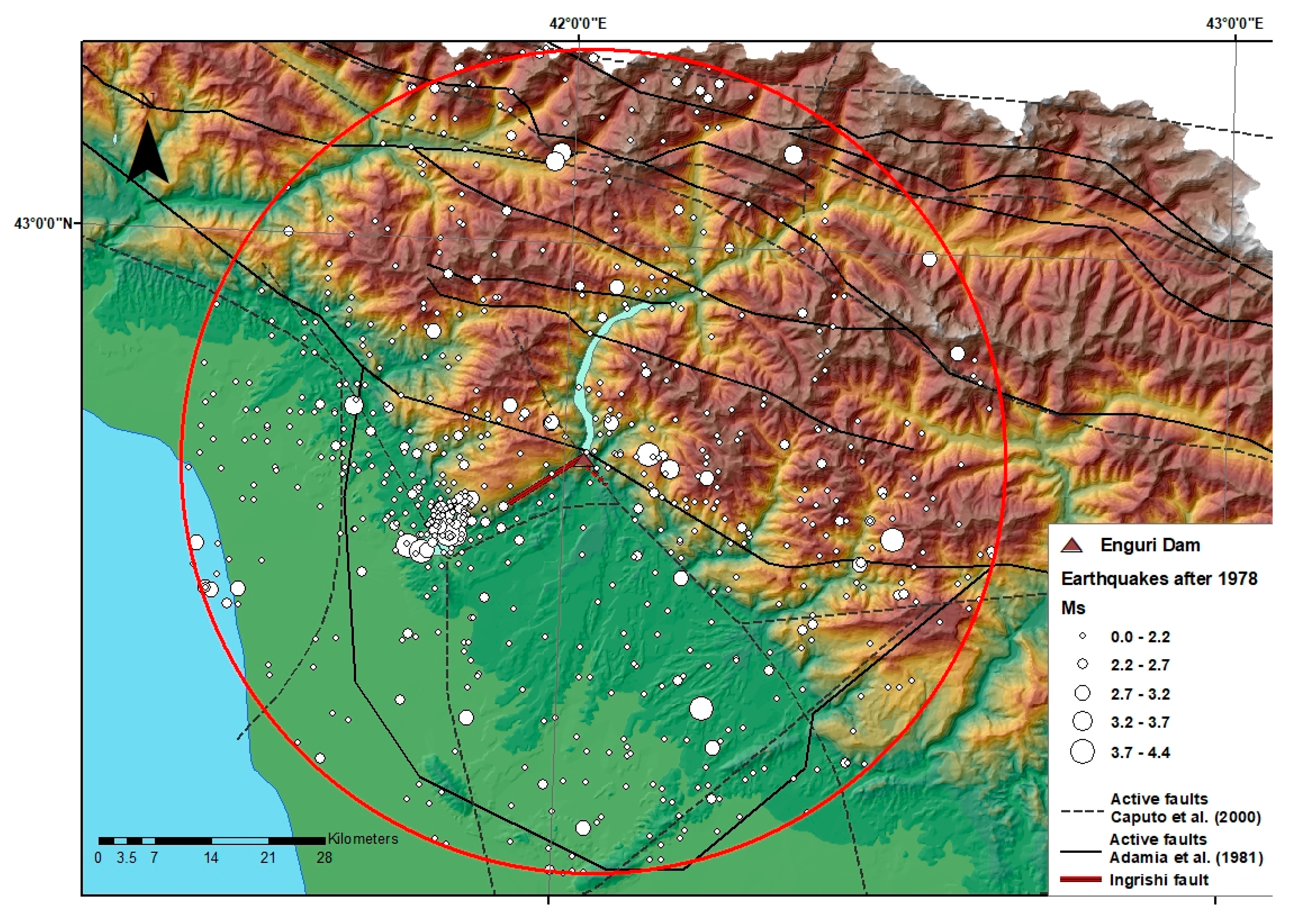
Figure 1.
Seismotectonic map of the Enguri area and investigated seismicity (white circles). The two models of active faults, as developed by Caputo e tal. [55] and Adamia et al. [24] are also indicated.
3. Seismicity Data
The earthquake catalog for the chosen area encompasses events spanning from 1978 to 2021. Various types of magnitude measurements have been employed to estimate the energetic parameters of earthquakes over different time intervals [45,56]. Up to 2003, the energetic parameters of earthquakes were assessed using surface waves (MLH/MS), primarily for moderate to strong earthquakes with , employing the regional calibration curve for MS [57,58]. During this period, for small to moderate earthquakes, the estimation was made in terms of energy class (K) [59]. When direct determination of MS was not feasible, event sizes were estimated according to Rautian (1964). In certain cases, additional measures such as MPV (magnitude estimated from the vertical component of P waves) and MC (magnitude estimated from coda waves) were considered. Since 2004, due to the restructuring of the Georgian seismic network, only local magnitude values (ML/Ml) were calculated for recorded earthquakes. The calculation of Mw was limited to earthquakes with ML greater than 4.5 [60]. In seismicity analysis, homogenizing earthquake catalogs is crucial. Utilizing conversion equations developed for national data [45,56,61] and regional data [62] allows for catalog harmonization in terms of Ms or Mw magnitude. Until 2003, the most common parameter for earthquake energy assessment was the energy class K. The conversion equation between Mw and K, based on limited data for Azerbaijan [61], and the conversion between Ms and K [63] establish stable correlations drawn from a broad range of Caucasian data. The conversion equation by Onur et al. [61] is applicable within a specific range of K, limiting its accuracy for small earthquakes (K < 9). Consequently, in this study, we opted to homogenize the catalog in terms of Ms. Since 2000, the Institute of Geophysics of I. Javakhishvili State University of Tbilisi (Georgia) has been dedicated to enhancing earthquake location accuracy for events with . The methodologies employed for recalculating kinematic parameters of earthquakes [60] have reduced the estimation error for depths to 2–3 km and epicentral coordinates of earthquakes with after 1956. For the Enguri dam area, the relocated event depths are more evenly distributed, with a prevalence of shallower depths (less than 15 km).
The seismic history of the investigated area reveals significant historical earthquakes (before 1900 AD) with intensities up to 9.5 on the MSK scale. Notable events include the Kvira earthquake in −1250 (Ms = 6.6), Nenskra-Abakura in 1100 (Ms = 7.0), Tsaishi in 1614 (Ms = 6.0), and Akiba in 1750 (Ms = 7.0) [64]. The strongest seismic event close to the Enguri dam site (within 7 km) before its construction occurred in 1930—the Samegrelo-Svaneti earthquake, with Ms = 4.8. The southeastern part of the dam exhibits high seismicity. In 1941, earthquake swarms occurred with main shocks of Ms = 4.7 and two shocks of Ms = 4.4. In 1957, the Martvili earthquake swarm featured three main shocks of Ms = 5.3 and two shocks of Ms = 5. High seismicity (i.e., large number of events) observed directly to the east of the dam is represented by the Zemo Samegrelo earthquake with a shock of Ms = 4.8 and numerous aftershocks lasting six months. A few small earthquakes are observed north of the dam along the current lake. Seismic activity increased after the filling of the Enguri reservoir began in 1978, particularly around the Gali water reservoir connected to the Enguri reservoir by a 16 km pressure-derivation tunnel. In 1979, a series of Rechkhi earthquakes occurred with foreshocks, two main shocks (Ms = 4.2 and 4.3), and several hundred aftershocks along the Gali water reservoir. The seismic activity in this area is ongoing, with events like the 2010 earthquake with Ms = 4.6. The new seismic network installed under the DAMAST project indicates high seismic activity in this area. From 2020 onwards, several hundred swarms of microearthquakes have occurred, although magnitude estimation for these events is challenging as they are recorded on only one station [54]. Figure 1 illustrates the investigated seismicity within a 50 km radius around the Enguri dam (from 1978 to 2021).
The Gutenberg–Richter (GR) law, as introduced by Gutenberg and Richter in 1944 [65], establishes a connection between the threshold magnitude and the number of earthquakes, denoted as N, with a magnitude equal to or greater than . This relationship is represented by the equation and is commonly employed to model the distribution of earthquake frequency as a function of magnitude. The two values of the GR law, namely a and b, signify, respectively, the level of seismic activity in a given region and the ratio of the number of smaller seismic events to that of larger ones. Accurate determination of the b-value is crucial for conducting reliable seismic hazard assessments [66,67]
In this paper, we estimated the b-value utilizing the maximum likelihood estimation (MLE) method [68]:
where is the mean of the magnitudes of the earthquakes, where is the bin size of the magnitude distribution and is the completeness magnitude, defined as the minimum magnitude above which all the events are recorded by the seismic network [69].
The estimation of the b-value depends on that of . To calculate , we utilized the goodness-of-fit test (GFT) method as described by Wiemer and Wyss (2000) [70]. In the GFT method, the observed distribution of magnitudes is compared with distributions synthetically generated with a-values and b-values estimated from the observed magnitudes as a function of the increasing cutoff magnitude . By defining R as the absolute difference within each magnitude bin between the number of earthquakes in the observed and synthetic distributions, we pinpoint the value of at the first , where the observed earthquake dataset for conforms to a straight-line pattern (in semilogarithmic scales) with a predetermined confidence level .
In this study, we investigated the earthquake activity from 1978 to 2021 in the Enguri area (Georgia), where a water reservoir is operating. These earthquakes were located within a 50 km radius from the center of the dam (see Figure 1), and their hypocenters had a maximum depth of 20 km.
4. Methods
4.1. The Periodogram Analysis
Given a time series , for , where N is the length of the series, its Discrete Fourier Transform (DFT) is defined as
where i is the imaginary unit and
The series can be obtained from its DFT by
The periodogram of is defined as
A peak in the periodogram at a frequency indicates a periodicity in the time series with period .
4.2. Schuster’s Spectrum
The Schuster test, introduced by Tanaka et al. in 2006 [71], was employed to investigate the potential influence of tidal forces on seismic activity. In the context of this test, when seismic activity follows a sinusoidal pattern with a period of T, it is assumed that the occurrence times of earthquakes can be described as a sinusoidal function. For each occurrence time of the k-th earthquake, denoted as , a phase angle can be associated, defined as . This effectively transforms the sequence of N occurrence times into a two-dimensional walk with unit-length steps, where the direction changes with the phase . If D represents the distance between the starting and ending points of this walk, the probability (p) that a distance greater than or equal to D can be reached by a uniformly distributed random two-dimensional walk corresponds to the likelihood that the occurrence times are randomly generated by a uniform seismicity rate. This probability is referred to as Schuster’s p-value and is calculated as follows:
The lower the Schuster’s p-value, the larger the probability of a periodicity at period T. Indicating as and the minimum and the maximum of the periods to be tested, the number M in Schuster’s tests is given by [72]
where usually . As demonstrated in [72], a periodicity T will be not due to chance if its Schuster p-value is lower than .
4.3. Empirical Mode Decomposition
The concept of empirical mode decomposition (EMD) was introduced by Huang et al. (1998) [73] as a method for decomposing a time series into so-called intrinsic mode functions (IMFs) that are characterized by two key conditions:
(a) Extremes and Zero-Crossings: The number of local extremes (maxima and minima) and zero-crossings in an IMF differ by at most one;
(b) Envelope Mean: At any given point, the mean value of the upper envelope (determined by local maxima) and the lower envelope (determined by local minima) is zero.
The process of decomposing a series into IMFs is accomplished through an iterative algorithm called the sifting algorithm:
(1) Connect all local maxima in the series with a cubic spline line to create the upper envelope, denoted as ;
(2) Connect all local minima in the series with a cubic spline line to create the lower envelope, denoted as ;
(3) Compute the mean envelope, denoted as , as the average of the upper and lower envelopes , and subtract this mean envelope from the original series, obtaining ;
(4) Check if satisfies the conditions to be an IMF; if these conditions are not satisfied, treat as the new series and return to step (1). Repeat the sifting process until an IMF is obtained;
(5) Denoting as the first IMF, subtract it from the original series and return to step (1);
(6) Once all the IMFs are obtained, the remaining part of the series, referred to as the residual, is simply obtained by removing all the found IMFs from the original series .
The entire decomposition process is expected to yield a finite number of IMFs.
There are variations of the EMD, such as ensemble empirical mode decomposition (EEMD) that mitigates the effect of undesired ’mode mixing’, which could impact the IMFs in the EMD [74].
5. Results
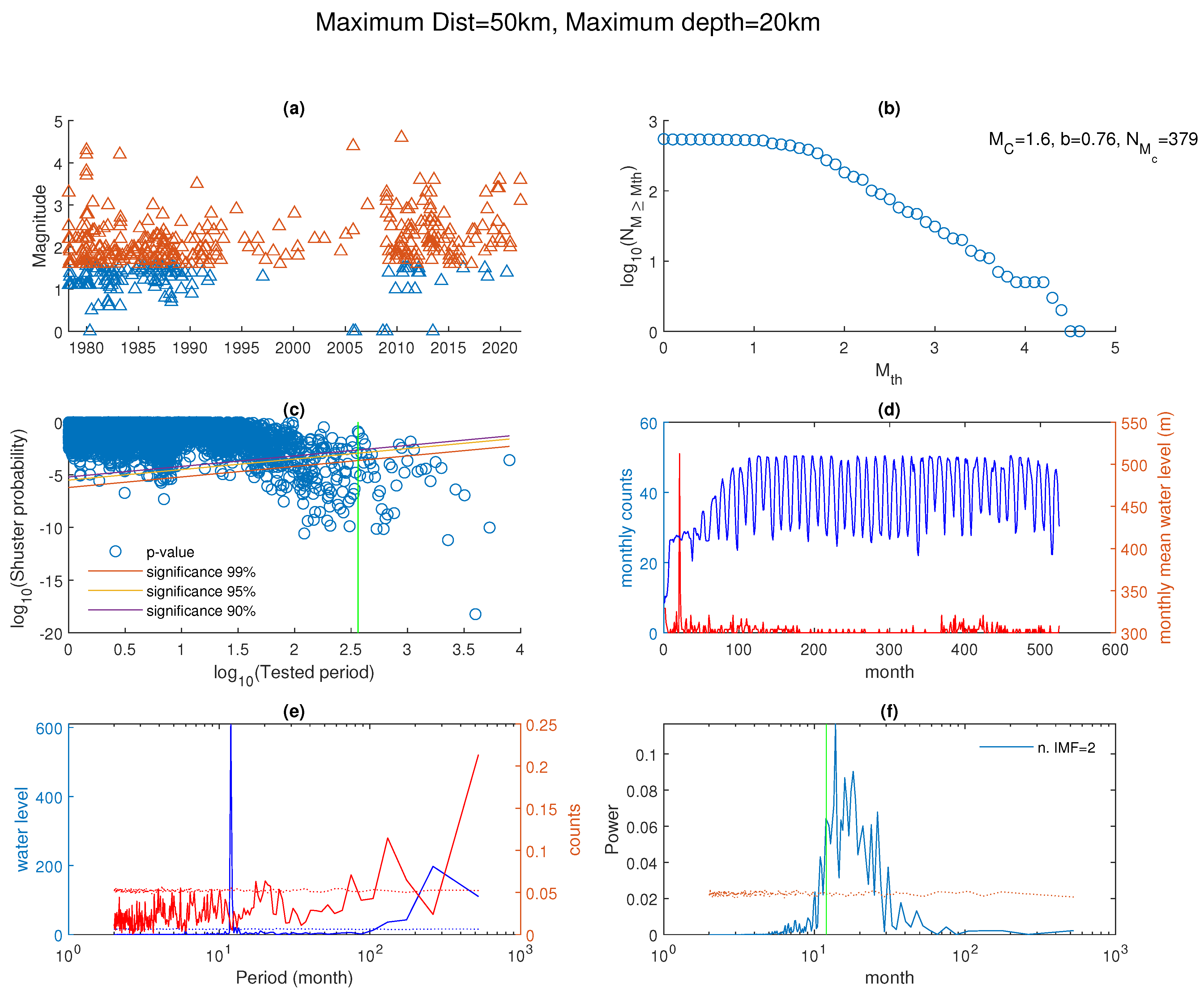
We investigated the spectral characteristics of the seismicity occurring around the Enguri water reservoir. The total number of recorded events in this study is 547 (Figure 2a).
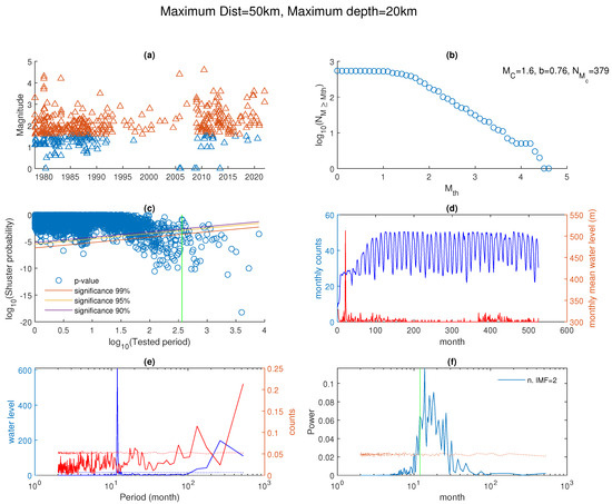
Figure 2.
(a) Time distribution of the earthquakes in the investigated area from 1978 to 2021. The maximum distance from the center of the dam is 50 km and the maximum depth is 20 km. The red triangles represent the earthquakes above the completeness magnitude. (b) Cumulative frequency–magnitude distribution. By applying the GFT method, the completeness magnitude = 1.6 and b = 0.76. (c) Schuster’s spectrum; the green vertical line marks the annual periodicity. (d) Monthly number of earthquakes and mean water level. (e) Periodograms of the monthly mean water level (blue) and the monthly earthquake counts (red). (f) Periodogram of IMF; the annual cycle is marked by the green vertical line. The red dotted line indicates the 95% confidence level.
We computed the frequency–magnitude distribution (see Figure 2b) and applied the GFT method with a confidence level of to determine the completeness magnitude, which was determined to be . Using Equation (1), we calculated a b-value of 0.76. Consequently, we filtered the dataset to include only those earthquakes with a magnitude , reducing the total number of earthquakes to 379, as indicated by the red triangles in Figure 2b. Subsequent analyses will be focused on this complete subset of earthquakes.
Figure 2c shows the Schuster spectrum of the analyzed earthquakes along with the lines of confidence at 90%, 95%, and 99%. For each tested period ranging from 1 day to the half of the entire period of investigation, the p-value (blue circles) was calculated. The Schuster spectrum of the chosen earthquake dataset reveals numerous significant periods at 99%, predominantly clustered around the annual cycle (indicated by the vertical green line) (Figure 2c).
Figure 2d depicts the temporal variation in the monthly number of earthquakes (with ) alongside the monthly mean water level of the Enguri reservoir. Besides the large monthly number of events occurring just after the beginning of the filling of the reservoir, the monthly variation in the number of earthquakes does not exceed five events/month, while the mean water level is modulated by a clear annual oscillation. Such oscillating behavior is also confirmed by the periodogram analysis. Figure 2e shows the periodogram of the monthly mean water level (blue) and that of the monthly counts (red), along with their respective 95% confidence lines (dotted). To calculate the 95% confidence value for each period, we employed the random shuffling method. This involved generating 1000 randomly permuted series. For each of these series, we calculated the periodogram. Subsequently, we obtained the distribution of periodogram values for each period, forming a confidence curve by enveloping all the 95th percentiles. A periodogram value is considered significant if it exceeds the 95% confidence curve. If the water level exhibits a noticeable and significant cycle over a one-year period, this pattern is not clearly observed in the monthly counts.
Thus, in order to disclose possible annual periodic patterns in the monthly counts of earthquakes, we utilized the empirical mode decomposition (EMD) method on the earthquake counts. Five MFs were generated by applying the sifting algorithm along with a residual component (depicted in Supplementary Figure S1). Following this, we computed the periodogram of each IMF, illustrated in Supplementary Figure S2. Among these five IMFs, the second one reveals a band of periodicities significant at the 95% confidence level (Figure 2f), with the maximal one closer to the annual cycle, corresponding to the periodic pattern that characterizes the oscillatory fluctuations in water level.
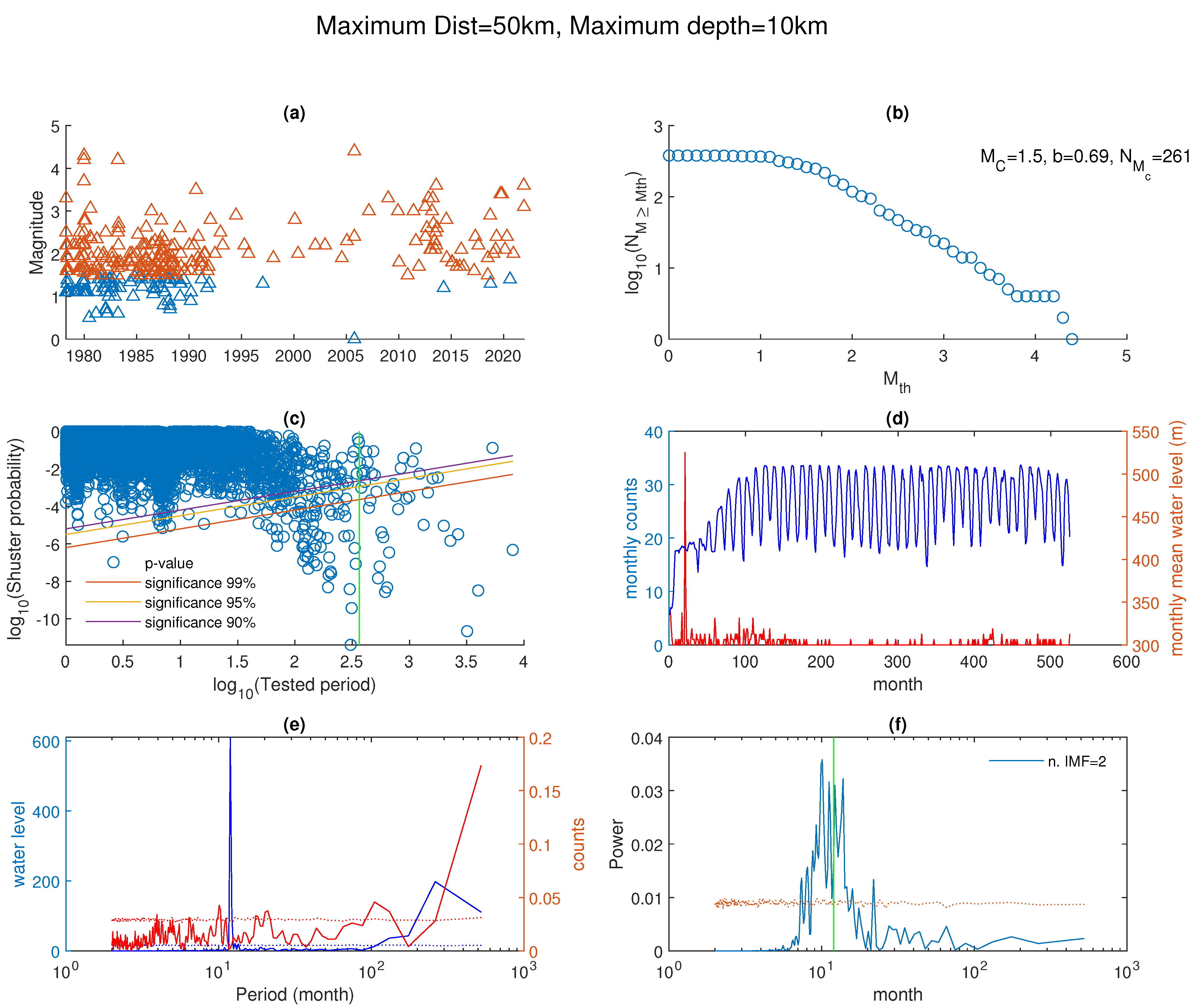
To examine the potential variations in the obtained results with depth, we replicated all the aforementioned analyses for shallower strata, using the dataset of events within a 50 km radius from the dam’s center but limited to a maximum depth of 10 km. This dataset comprises a total of 380 events (Figure 3a). With a completeness magnitude of 1.5 and a b-value of 0.69, the complete dataset comprises 261 events (Figure 3b). The Schuster spectrum shows many significant periods at 99% (Figure 3c); however, it is really striking that the most significant period that corresponds to the lowest p-value is very close to the annual periodicity (indicated by the green vertical line). Such a result clearly indicates that this shallower seismicity is significantly modulated by the annual cycle.
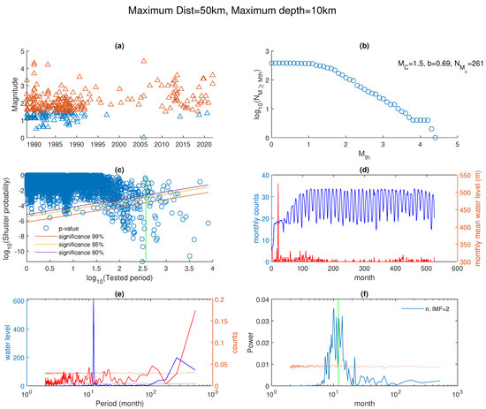
Figure 3.
(a) Time distribution of the earthquakes in the investigated area from 1978 to 2021. The maximum distance from the center of the dam is 50 km and the maximum depth is 10 km. The red triangles represent the earthquakes above the completeness magnitude. (b) Cumulative frequency–magnitude distribution. By applying the GFT method, the completeness magnitude = 1.5 and b = 0.69. (c) Schuster’s spectrum; the green vertical line marks the annual periodicity. (d) Monthly number of earthquakes and mean water level. (e) Periodograms of the monthly mean water level (blue) and the monthly earthquake counts (red). (f) Periodogram of IMF; the annual cycle is marked by the green vertical line. The red dotted line indicates the 95% confidence level.
The pattern of the mean monthly earthquake counts closely resembles that of the dataset with a maximum depth of 20 km (Figure 3d). Their periodograms display a distinct annual cycle for the water level, yet this pattern is not apparent in the earthquake counts (Figure 3e). Applying the EMD method to the monthly count of events (Supplementary Figures S3 and S4) allows the identification of the annual cycle within the second IMF (Figure 3f). The spectral content of the second IMF of this dataset is primarily centered around the annual cycle, while that of the second IMF of the previous dataset (maximum depth less than 20 km) is more shifted towards higher periods.
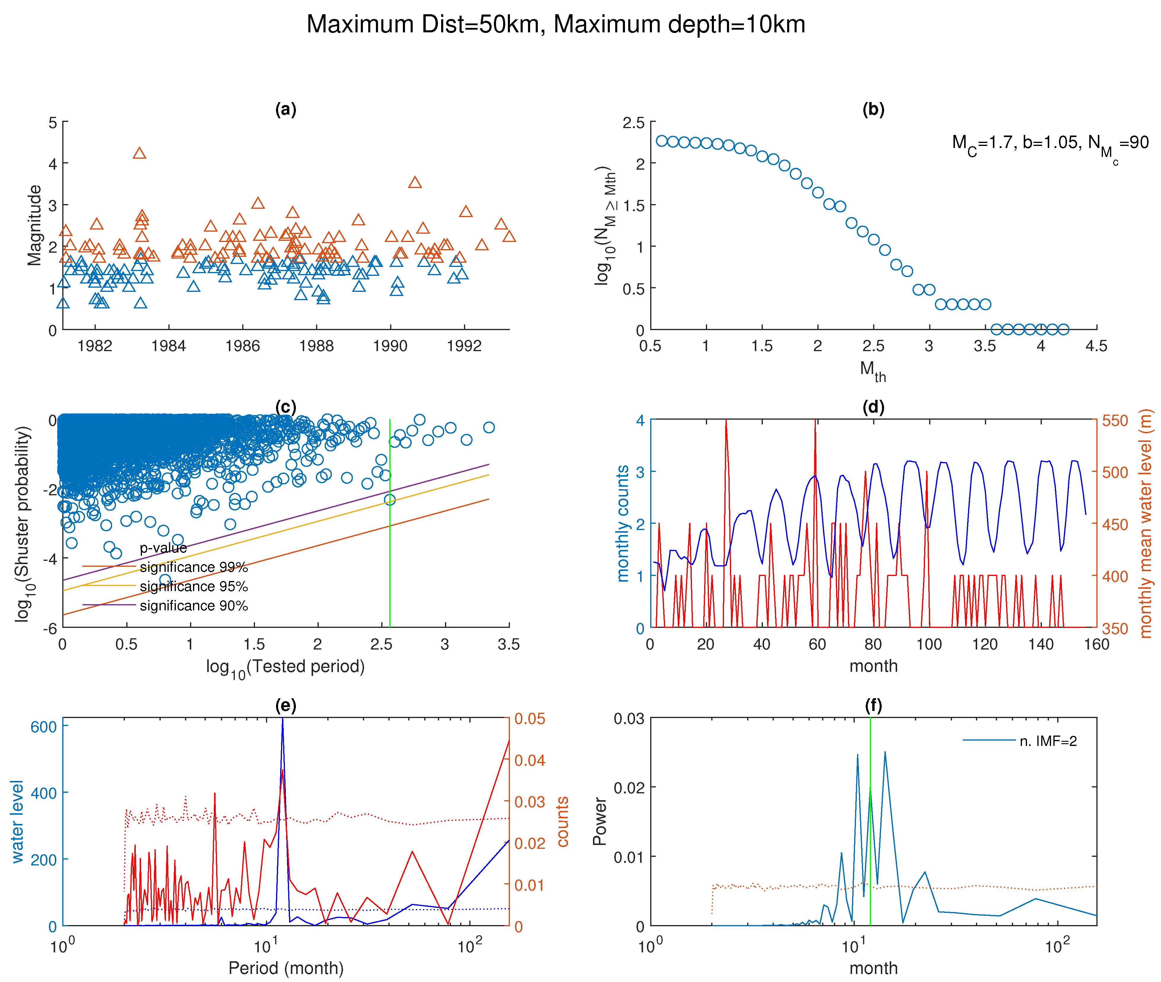
The temporal occurrence of earthquakes exhibits a burst of activity between 1978 and 1980 and a certain sparsity after 1993. To ascertain whether these two observed phenomena may have impacted the results, we conducted an analysis specifically focusing on the period between 1981 and 1993, which appears to be rather stationary. Figure 4 presents the results of our analysis. Examining the frequency–magnitude distribution reveals completeness in the seismic catalog for magnitudes greater than or equal to 1.7, with a Gutenberg–Richter law b-value of 1.05 (Figure 4a). The Schuster spectrum (Figure 4c) indicates a significant periodicity at 1 year with a confidence level of 95%. The monthly counts of earthquakes (Figure 4d) are characterized by a yearly oscillation, which is very clearly shown in the periodogram (Figure 4e) and in the second IMF’s periodogram (Figure 4f).

Figure 4.
(a) Time distribution of the earthquakes in the investigated area from 1981 to 1993. The maximum distance from the center of the dam is 50 km and the maximum depth is 10 km. The red triangles represent the earthquakes above the completeness magnitude. (b) Cumulative frequency–magnitude distribution. By applying the GFT method, the completeness magnitude = 1.7 and b = 1.05. (c) Schuster’s spectrum; the green vertical line marks the annual periodicity. (d) Monthly number of earthquakes and mean water level. (e) Periodograms of the monthly mean water level (blue) and the monthly earthquake counts (red). (f) Periodogram of IMF; the annual cycle is marked by the green vertical line. The red dotted line indicates the 95% confidence level.
This outcome further reinforces the possibility that seismic activity around the Enguri reservoir might be influenced by the loading and unloading cycles of water reservoir operations and could be considered a contributing source of the seismic occurrences, although it is evident that the impact of water level fluctuations is significantly more pronounced in the shallower strata compared to the deeper ones.
6. Conclusions
In this research, we performed a spectral analysis on the temporal patterns of instrumental seismic activity in the Enguri area of Georgia from 1978 to 2021. The earthquake dataset underwent examination through Schuster’s spectrum analysis, periodogram analysis, and empirical mode decomposition analysis.
Our findings indicate that seismicity in the vicinity of the dam may be attributable to fluctuations in water levels, influenced by the annual cycle of loading and unloading operations of the water reservoir. Notably, the impact of water fluctuations is more pronounced in shallower strata compared to deeper ones. This observation suggests that earthquakes occurring at deeper levels may primarily result from tectonic forces, whereas those at shallower depths may be predominantly triggered by reservoir-induced factors.
Supplementary Materials
The following supporting information can be downloaded at: https://www.mdpi.com/article/10.3390/geosciences14010022/s1.
Author Contributions
Conceptualization, L.T.; methodology, L.T.; software, L.T.; formal analysis, L.T.; investigation, L.T., T.C. and N.T.; data curation, N.T.; writing—original draft preparation, L.T.; writing—review and editing, L.T., T.C., N.T. and V.L.; visualization, L.T. and N.T.; project administration, V.L. and T.C.; funding acquisition, V.L. and T.C. All authors have read and agreed to the published version of the manuscript.
Funding
This research was funded by National Research Council (93C23000100005), by Shota Rustaveli National Science Foundation of Georgia (FR-21-20840).
Data Availability Statement
The data presented in this study are available on request.
Conflicts of Interest
The authors declare no conflicts of interest.
References
- Gupta, H.K. A review of recent studies of triggered earthquakes by artificial water reservoirs with special emphasis on earthquakes in Koyna, India. Earth Sci. Rev. 2002, 58, 279–310. [Google Scholar] [CrossRef]
- Bhaskara Rao, V.; Satyanarayana Murty, B.; Satyanarayana Murty, A. Some geological and geophysical aspects of the Koyna (India) earthquake, December 1967. Tectonophysics 1969, 7, 265–271. [Google Scholar]
- Gupta, H.K.; Rastogi, B.K.; Narain, H. The Koyna earthquake of December 10, 1967: A multiple seismic event. Bull. Seismol. Soc. Am. 1971, 61, 167–176. [Google Scholar] [CrossRef]
- Agrawal, P.N. December 11, 1967 Koyna earthquake and reservoir filling. Bull. Seismol. Soc. Am. 1972, 62, 661–662. [Google Scholar] [CrossRef]
- Talwani, P. Seismotectonics of the Koyna-Warna area, India. Pure Appl. Geophys. 1997, 150, 511–550. [Google Scholar] [CrossRef]
- Telesca, L. Analysis of the cross-correlation between seismicity and water level in Koyna area (India). Bull. Seismol. Soc. Am. 2010, 100, 2317–2321. [Google Scholar] [CrossRef]
- Simpson, D.W.; Negmatullaev, S.K. Induced seismicity at Nurek Reservoir, Tadjikistan, USSR. Bull. Seismol. Soc. Am. 1981, 71, 1561–1586. [Google Scholar]
- Leblanc, G.; Anglin, F. Induced seismicity at the Manic 3 reservoir, Quebec. Bull. Seismol. Soc. Am. 1978, 68, 1469–1485. [Google Scholar] [CrossRef]
- Gahalaut, K.; Gahalaut, V.; Pandey, M. A new case of reservoir-triggered seismicity: Govind Ballav Pant reservoir (Rihand dam), central India. Tectonophysics 2007, 439, 171–178. [Google Scholar] [CrossRef]
- Gough, D.; Gough, W. Load-induced earthquakes at Lake Kariba, 2. Geophys. J. 1970, 79, 101. [Google Scholar] [CrossRef]
- Gupta, H.; Rastogi, B. Dams and Earthquakes; Elsevier: Amsterdam, The Netherlands, 1976; p. 229. [Google Scholar]
- Gupta, H. Preface. In Reservoir-Induced Earthquakes; Elsevier: New York, NY, USA, 1992; Volume 64. [Google Scholar]
- Liu, S.; Xu, L.; Talwani, P. Reservoir-induced seismicity in the Danjiangkou Reservoir: A quantitative analysis. Geophys. J. Int. 2011, 185, 514–528. [Google Scholar] [CrossRef]
- Rajendran, K.; Harish, C.; Kumaraswamy, S. Re-Evaluation of Earthquake Data from Koyna—Warna Region: Phase I; Technical Report; Department of Science and Technology: Trivandrum, India, 1996. [Google Scholar]
- Rajendran, K.; Harish, C. Mechanism of triggered seismicity at Koyna: An assessment based on relocated earthquakes during 1983–1993. Curr. Sci. 2000, 79, 358–363. [Google Scholar]
- Nascimento, A.; Cowie, P.; Lunn, R.; Pearce, R. Spatio-temporal evolution of induced seismicity at Acu reservoir, NE Brazil. Geophys. J. Int. 2004, 158, 1041–1052. [Google Scholar] [CrossRef]
- Gupta, H.; Shashidhar, D.; Pereira, M.; Purnachandra Rao, N.; Kousalya, M.; Satyanarayana, H.; Saha, S.; Babu Naik, R.; Dimri, V. A new zone of seismic activity at Koyna, India. J. Geol. Soc. India 2007, 69, 1136–1137. [Google Scholar]
- Gupta, H.; Rao, N.; Roy, S.; Arora, K.; Tiwari, V.; Patro, P.; Satyanarayana, H.; Shashidhar, D.; Mallika, K.; Akkiraju, V. Investigations related to scientific deep drilling to study reservoir-triggered earthquakes at Koyna, India. Int. J. Earth Sci. 2015, 10, 1511–1522. [Google Scholar] [CrossRef]
- Mikhailov, V.; Arora, K.; Ponomarev, A.; Srinagesh, D.; Smirnov, V.; Chadha, R. Reservoir-induced seismicity in the Koyna–Warna region, India: Overview of the recent results and hypotheses. Izv. Phys. Solid Earth 2017, 53, 518–529. [Google Scholar] [CrossRef]
- Valoroso, L.; Improta, L.; Chiaraluce, L.; Di Stefano, R.; Ferranti, L.; Govoni, A.; Chiarabba, C. Active faults and induced seismicity in the Val d’Agri area (Southern Apennines, Italy). Geophys. J. Int. 2009, 178, 488–502. [Google Scholar] [CrossRef]
- Telesca, L.; Kadirov, F.; Yetirmishli, G.; Safarov, R.; Babayev, G.; Islamova, S.; Kazimova, S. Analysis of the relationship between water level temporal changes and seismicity in the Mingechevir reservoir (Azerbaijan). J. Seismol. 2020, 24, 937–952. [Google Scholar] [CrossRef]
- Telesca, L.; Thai, A.T.; Cao, D.T.; Ha, T.G. Spectral evidence for reservoir triggered seismicity at Song Tranh 2 Reservoir (Vietnam). Pure Appl. Geophys. 2021, 178, 3817–3828. [Google Scholar] [CrossRef]
- Gupta, H.; Rastogi, B.; Narain, H. Common features of the reservoir-associated seismic activities. Bull. Seismol. Soc. Am. 1972, 62, 481–492. [Google Scholar] [CrossRef]
- Adamia, S.A.; Chkhotua, T.; Kekelia, M.; Lordkipanidze, M.; Shavishvili, I.; Zakariadze, G. Tectonics of the Caucasus and adjoining regions: Implications for the evolution of the Tethys ocean. J. Struct. Geol. 1981, 3, 437–447. [Google Scholar] [CrossRef]
- Adamia, S.; Alania, V.; Chabukiani, A.; Chichua, G.; Enukidze, O.; Sadradze, N. Evolution of the late Cenozoic basins of Georgia (SW Caucasus): A review. Geol. Soc. Lond. Spec. Publ. 2010, 340, 239–259. [Google Scholar] [CrossRef]
- Jackson, J.; Ambraseys, N.; Giardini, D.; Balassanian, S. Convergence between Eurasia and Arabia in eastern Turkey and the Caucasus. Hist. Prehist. Earthquakes Cauc. 1997, 28, 79–90. [Google Scholar]
- Banks, C.J.; Robinson, A.G.; Williams, M.P. Structure and Regional Tectonics of the Achara-Trialet Fold Belt and the Adjacent Rioni and Kartli Foreland Basins, Republic of Georgia; American Association of Petroleum Geologists: Tulsa, OK, USA, 1997; pp. 331–346. [Google Scholar]
- Smith, A.G. Alpine deformation and the oceanic areas of the Tethys, Mediterranean, and Atlantic. Geol. Soc. Am. Bull. 1971, 82, 2039–2070. [Google Scholar] [CrossRef]
- Dewey, J.F.; Pitaman, W.C.; Ryan, W.B.; Bonnin, J. Plate tectonics and the evolution of the Alpine system. Geol. Soc. Am. Bull. 1973, 84, 3137–3180. [Google Scholar] [CrossRef]
- Khain, V. Structure and main stages in the tectonomagmatic development of the Caucasus: An attempt at geodynamic interpretation. Am. J. Sci. 1975, 275, 131–156. [Google Scholar]
- Pearce, J.A.; Bender, J.; De Long, S.; Kidd, W.; Low, P.; Güner, Y.; Saroglu, F.; Yilmaz, Y.; Moorbath, S.; Mitchell, J. Genesis of collision volcanism in Eastern Anatolia, Turkey. J. Volcanol. Geotherm. Res. 1990, 44, 189–229. [Google Scholar] [CrossRef]
- Mosar, J.; Kangarli, T.; Bochud, M.; Glasmacher, U.A.; Rast, A.; Brunet, M.F.; Sosson, M. Cenozoic-recent tectonics and uplift in the greater Caucasus: A perspective from Azerbaijan. Geol. Soc. Spec. Publ. 2010, 340, 261–280. [Google Scholar] [CrossRef]
- Sosson, M.; Rolland, Y.; Müller, C.; Danelian, T.; Melkonyan, R.; Kekelia, S.; Adamia, S.; Babazadeh, V.; Kangarli, T.; Avagyan, A.; et al. Subductions, obduction and collision in the lesser Caucasus (Armenia, Azerbaijan, Georgia), new insights. Geol. Soc. Spec. Publ. 2010, 340, 329–352. [Google Scholar] [CrossRef]
- Martin, R.J.; Gulen, L.; Sun, Y.; Toksoz, M. The Crustal and Mantle Velocity Structure in Central Asia from 3D Travel Time Tomography; Technical Report; New England Research Inc. (Veterans Affairs): White River Junction, VT, USA, 2010. [Google Scholar]
- Mcclusky, S.; Balassanian, S.; Barka, A.; Demir, C.; Ergintav, S.; Georgiev, I.; Gurkan, O.; Hamburger, M.; Hurst, K.; Kahle, H.; et al. Global positioning system constraints on plate kinematics and dynamics in the eastern Mediterranean and Caucasus. J. Geophys. Res. Solid Earth 2000, 105, 5695–5719. [Google Scholar] [CrossRef]
- Allen, M.; Jackson, J.; Walker, R. Late Cenozoic reorganization of the Arabia-Eurasia collision and the comparison of short-term and long-term deformation rates. Tectonics 2004, 23, TC2008. [Google Scholar] [CrossRef]
- Reilinger, R.; McClusky, S.; Vernant, P.; Lawrence, S.; Ergintav, S.; Cakmak, R.; Ozener, H.; Kadirov, F.; Guliev, I.; Stepanyan, R.; et al. GPS constraints on continental deformation in the Africa-Arabia-Eurasia continental collision zone and implications for the dynamics of plate interactions. J. Geophys. Res. Solid Earth 2006, 11, B05411. [Google Scholar] [CrossRef]
- Tan, O.; Taymaz, T. Active tectonics of the Caucasus: Earthquake source mechanisms and rupture histories obtained from inversion of teleseismic body waveforms. Spec. Pap. Geol. Soc. Am. 2006, 409, 531. [Google Scholar]
- Kadirov, F.; Mammadov, S.; Reilinger, R.; McClusky, S. Some new data on modern tectonic deformation and active faulting in Azerbaijan (according to Global Positioning System measurements). Proc. Azerbaijan Natl. Acad. Sci. Proc. Sci. Earth 2008, 1, 82–88. [Google Scholar]
- Kadirov, F.; Gadirov, A.; Abdullayev, N. Gravity modelling of the regional profile across South Caspian basin and tectonic implications. In The Modern Problems of Geology and Geophysics of Eastern Caucasus and the South Caspian Depression; Nafta-Press: Bonn, Germany, 2012. [Google Scholar]
- Pasquarè, F.; Tormey, D.; Vezzoli, L.; Okrostsvaridze, A.; Tutberidze, B. Mitigating the consequences of extreme events on strategic facilities: Evaluation of volcanic and seismic risk affecting the Caspian oil and gas pipelines in the Republic of Georgia. J. Environ. Manag. 2011, 92, 1774–1782. [Google Scholar] [CrossRef]
- Tibaldi, A.; Alania, V.; Bonali, F.; Enukidze, O.; Tsereteli, N.; Kvavadze, N.; Varazanashvili, O. Active inversion tectonics, simple shear folding and back-thrusting at Rioni Basin, Georgia. J. Struct. Geol. 2017, 96, 35–53. [Google Scholar] [CrossRef]
- Tibaldi, A.; Russo, E.; Bonali, F.; Alania, V.; Chabukiani, A.; Enukidze, O.; Tsereteli, N. 3-d anatomy of an active fault-propagation fold: A multidisciplinary case study from Tsaishi, western Caucasus (Georgia). Tectonophysics 2017, 717, 253–269. [Google Scholar] [CrossRef]
- Tibaldi, A.; Bonali, F.; Russo, E.; Mariotto, F.P. Structural development and stress evolution of an arcuate fold-and-thrust system, southwestern greater Caucasus, republic of Georgia. J. Asian Earth Sci. 2018, 156, 226–245. [Google Scholar] [CrossRef]
- Tibaldi, A.; Tsereteli, N.; Varazanashvili, O.; Babayev, G.; Barth, A.; Mumladze, T.; Bonali, F.; Russo, E.; Kadirov, F.; Yetirmishli, G.; et al. Active stress field and fault kinematics of the greater Caucasus. J. Asian Earth Sci. 2020, 188, 104108. [Google Scholar] [CrossRef]
- DeMets, C.; Gordon, R.; Argus, D.; Stein, S. Current plate motions. Geophys. J. Int. 1990, 101, 425–478. [Google Scholar] [CrossRef]
- DeMets, C.; Gordon, R.; Argus, D.; Stein, S. Effect of recent revisions to the geomagnetic reversal time scale on estimates of current plate motions. Geophys. Res. Lett. 1994, 21, 2191–2194. [Google Scholar] [CrossRef]
- Triep, E.; Abers, G.; Lerner-Lam, A.; Mishatkin, V.; Zakharchenko, N.; Starovoit, O. Active thrust front of the greater Caucasus: The April 29, 1991, Racha earthquake sequence and its tectonic implications. J. Geophys. Res. Solid Earth 1995, 100, 4011–4033. [Google Scholar] [CrossRef]
- Sokhadze, G.; Floyd, M.; Godoladze, T.; King, R.; Cowgill, E.; Javakhishvili, Z.; Hahubia, G.; Reilinger, R. Active convergence between the lesser and greater Caucasus in Georgia: Constraints on the tectonic evolution of the lesser-greater Caucasus continental collision. Earth Planet. Sci. Lett. 2018, 481, 154–161. [Google Scholar] [CrossRef]
- Reilinger, R.; McClusky, S.; Oral, M.; King, R.; Toksoz, M.; Barka, A.; Kinik, I.; Lenk, O.; Sanli, I. Global positioning system measurements of present-day crustal movements in the Arabia-Africa-Eurasia plate collision zone. J. Geophys. Res. Solid Earth 1997, 102, 9983–9999. [Google Scholar] [CrossRef]
- Shevchenko, V.; Guseva, T.; Lukk, A.; Mishin, A.; Prilepin, M.; Reilinger, R.; Hamburger, M.; Shempelev, A.; Yunga, S. Recent geodynamics of the Caucasus mountains from GPS and seismological evidence. Izv. Phys. Solid Earth 1999, 35, 691–704. [Google Scholar]
- Guliev, I.; Kadirov, F.; Reilinger, R.; Gasanov, R.; Mamedov, A. Active tectonics in Azerbaijan based on geodetic, gravimetric, and seismic data. Dokl. Earth Sci. 2002, 383, 174–177. [Google Scholar]
- Aktuğ, B.; Meherremov, E.; Kurt, M.; Özdemir, S.; Esedov, N.; Lenk, O. GPS constraints on the deformation of Azerbaijan and surrounding regions. J. Geodyn. 2013, 67, 40–45. [Google Scholar] [CrossRef]
- Karamzadeh, N.; Tsereteli, N.; Gaucher, E.; Tugushi, N.; Shubladze, T.; Varazanashvili, O.; Rietbrock, A. Seismological study around the Enguri dam reservoir (Georgia) based on old catalogs and ongoing monitoring. J. Seismol. 2023, 27, 953–977. [Google Scholar] [CrossRef]
- Caputo, M.; Gamkrelidze, I.; Malvezzi, V.; Sgrigna, V.; Shengelaia, G.; Zilpimiani, D. Geostructural basis and geophysical investigations for the seismic hazard assessment and prediction in the Caucasus. Il Nuovo Cimento C 2000, 23, 191–216. [Google Scholar]
- Tsereteli, N.; Danciu, L.; Varazanashvili, O.; Sesetyan, K.; Qajaia, L.; Sharia, T.; Svanadze, D.; Khvedelidze, I. The 2020 national seismic hazard model for Georgia (Sakartvelo). In Building Knowledge for Geohazard Assess Management in the Caucasus and other Orogenic Regions; Springer: Dordrecht, The Netherlands, 2021; pp. 131–168. [Google Scholar]
- Kondorskaya, N.V.; Shebalin, N.V. New Catalog of Strong Earthquakes in the USSR from Ancient Times through 1977; World Data Center A for Solid Earth Geophysics; EDIS: Boulder, CO, USA, 1982; p. 608. [Google Scholar]
- Vanek, I.; Zatopek, A.; Karnik, V.; Kondorskaya, N.V.; Riznichenko, Y.V.; Savarensky, E.F.; Solovyev, S.L.; Shebalin, N.V. Standardization of Magnitude Scales. IZV. AN SSSR Ser. Geophys. 1962, 1, 153–158. [Google Scholar]
- Rautian, T.G.; Khalturin, V.I.; Fujita, K.; Mackey, K.G.; Kendall, A.D. Origins and Methodology of the Russian Energy K-Class System and Its Relationship to Magnitude Scales. Seismol. Res. Lett. 2007, 78, 579–590. [Google Scholar] [CrossRef]
- Tsereteli, N.; Tibaldi, A.; Alania, V.; Gventsadse, A.; Enukidze, O.; Varazanashvili, O.; Müller, B. Active tectonics of central-western Caucasus, Georgia. Tectonophysics 2016, 691, 328–344. [Google Scholar] [CrossRef]
- Onur, T.; Gok, R.; Godoladze, T.; Gunia, I.; Boichenko, G.; Buzaladze, A.; Tumanova, N.; Dzmanashvili, M.; Sukhishvili, L.; Javakishvili, Z.; et al. Probabilistic Seismic Hazard Assessment Using Legacy Data in Georgia. Seismol. Res. Lett. 2020, 91, 1500–1517. [Google Scholar] [CrossRef]
- Zare, M.; Amini, H.; Yazdi, P.; Sesetyan, K.; Demircioglu, M.B.; Kalafat, D.; Erdik, M.; Giardini, D.; Khan, M.A.; Tsereteli, N. Recent developments of the Middle East catalog. J. Seismol. 2014, 18, 749–772. [Google Scholar] [CrossRef]
- Rautian, T. Determination of earthquake energy at a distance to 3000 km. Eksp Seismika Trudy IFZ AN SSSR 1964, 32, 199. [Google Scholar]
- Varazanashvili, O.; Tsereteli, N.; Bonali, F.; Arabidze, V.; Russo, E.; Pasquaré Mariotto, F.; Gogoladze, Z.; Tibaldi, A.; Kvavadze, N.; Oppizzi, P. GeoInt: The first macroseismic intensity database for the Republic of Georgia. J. Seismol. 2018, 22, 625–667. [Google Scholar] [CrossRef]
- Gutenberg, R.; Richter, C.F. Frequency of earthquakes in California. Bull. Seismol. Soc. Am. 1944, 34, 185–188. [Google Scholar] [CrossRef]
- Scholz, C.H. The frequency-magnitude relation of microfracturing in rock and its relation to earthquakes. Bull. Seismol. Soc. Am. 1968, 58, 399–415. [Google Scholar] [CrossRef]
- Wyss, M. Towards a physical understanding of the earthquake frequency distribution. Geophys. J. R. Astron. Soc. 1973, 31, 341–359. [Google Scholar] [CrossRef]
- Aki, K. Maximum likelihood estimate of b in the formula log(N)=a-bM and its confidence limits. Bull. Earthq. Res. Inst. Univ. Tokyo 1965, 43, 237–239. [Google Scholar]
- Utsu, T. Representation and analysis of the earthquake size distribution: A historical review and some new approaches. Pageoph 1999, 155, 509–535. [Google Scholar] [CrossRef]
- Wiemer, S.; Wyss, M. Minimum magnitude of completeness in earthquake catalogs: Examples from Alaska, the Western United States, and Japan. Bull. Seismol. Soc. Am. 2000, 90, 859–869. [Google Scholar] [CrossRef]
- Tanaka, S.; Sato, H.; Matsumura, S.; Ohtake, M. Tidal triggering of earthquakes in the subducting Philippine Sea plate beneath the locked zone of the plate interface in the Tokai region, Japan. Tectonophysics 2006, 417, 69–80. [Google Scholar] [CrossRef]
- Ader, T.J.; Avouac, J.P. Detecting periodicities and declustering in earthquake catalogs using the Schuster spectrum, application to Himalayan seismicity. Earth Planet. Sci. Lett. 2013, 377–378, 97–105. [Google Scholar] [CrossRef]
- Huang, N.E.; Shen, Z.; Long, S.R.; Wu, M.L.; Shih, H.H.; Zheng, Q.; Yen, N.C.; Tung, C.C.; Liu, H.H. The empirical mode decomposition and Hilbert spectrum for nonlinear and non-stationary time series analysis. Proc. Roy. Soc. Lond. A 1998, 454, 903–995. [Google Scholar] [CrossRef]
- Colominas, M.A.; Schlotthauer, G.; Torres, M.E. Improved complete ensemble EMD: A suitable tool for biomedical signal processing. Biomed. Signal Process. Control. 2014, 14, 19–29. [Google Scholar] [CrossRef]
Disclaimer/Publisher’s Note: The statements, opinions and data contained in all publications are solely those of the individual author(s) and contributor(s) and not of MDPI and/or the editor(s). MDPI and/or the editor(s) disclaim responsibility for any injury to people or property resulting from any ideas, methods, instructions or products referred to in the content. |
© 2024 by the authors. Licensee MDPI, Basel, Switzerland. This article is an open access article distributed under the terms and conditions of the Creative Commons Attribution (CC BY) license (https://creativecommons.org/licenses/by/4.0/).