Application of Experimental Configurations of Seismic and Electric Tomographic Techniques to the Investigation of Complex Geological Structures

Abstract

The main purpose of this study is the subsurface investigation of two complex geological environments focusing on the improvement of data acquisition and processing parameters regarding electric and seismic tomographic techniques. Two different study areas, in central–east Peloponnese and SE Attica, were selected, where detailed geological mapping and surface geophysical survey were carried out. The applied geophysical survey included the application of electrical resistivity tomography (ERT), seismic refraction tomography (SRT) and ground penetrating radar (GPR). The geoelectrical measurements were acquired with different arrays and electrode configurations. Moreover, various types of seismic sources were used at seventeen shot locations along the seismic arrays. For the processing of geoelectrical data, clustered datasets were created, increasing the depth of investigation and discriminatory capability. The seismic data processing included the following: (a) the creation of synthetic models and seismic records to determine the effectiveness and capabilities of the technique, (b) spectral analysis of the seismic records to determine the optimal seismic source type and (c) inversion of the field data to create representative subsurface velocity models. The results of the two techniques successfully delineated the complex subsurface structure that characterizes these two geological environments. The application of the ERT combined with the SRT are the two dominant, high-resolution techniques for the elucidation of complex subsurface structures.

1. Introduction

Subsurface investigation of complex geological environments has always been a major challenge for near-surface applied geophysics. A complex geological environment refers to an area where various geological factors interact in complicated processes, resulting in a dynamic environment. These environments usually consist of various geological formations, usually succeeding each other over a relatively short distance. They are characterized by the presence of extensional and compressional tectonic structures (faults, folds, overthrusts, detachments) due to the multiple deformational phases that have undergone. In addition to the tectonic causes, the exposure of the geological formations to exogenous and endogenous processes, such as erosion, weathering, faulting, magmatism and hydrothermal fluid circulation, further contributes to the complexity of the geological environment. All the above processes pose major challenges regarding the investigation and interpretation of such environments.

One-dimensional (1D) geophysical techniques, such as transient electromagnetics (TEM), borehole logging and vertical electrical sounding (VES), are not frequently used for subsurface investigation in complex geological environments due to the presence of strong lateral variations [1,2]. Moreover, the high-resolution shallow seismic reflection method often gets affected, regarding the data quality, by diffraction and scattering phenomena, multiple reflections and unsuccessful utilization of migration techniques due to the strong near-surface velocity contrasts and lateral velocity variations in fault zones [3,4].

Among several geophysical methods, electrical resistivity tomography (ERT) is a high-resolution and effective technique, capable of producing 2D or/and 3D subsurface resistivity distributions [5,6,7], which can typically be correlated with spatial variations in the lithological composition and the presence of tectonic structures in the investigated subsurface section. It has been widely applied to gain information about the location and structural characteristics of near-surface fault zones, their effective depth and to estimate the width of the affected zone [8,9,10,11]. Furthermore, ERT has been applied in complex geological environments for the delineation of conductive [12,13] and weathered zones [14], as well as for geotechnical purposes regarding the investigation of subsurface air-filled voids, fractures and bedrock depth [15,16,17].

The seismic refraction method is a widely applied geophysical method for near-surface investigations. Conventional seismic refraction processing techniques (intercept time and delay time-based methodologies) fail to reveal the actual subsurface structure in complex environments since they utilize oversimplified geometry by dividing the substratum into discrete layers of constant velocity. However, more advanced and complex inversion algorithms have established the seismic refraction tomography (SRT) technique as an important geophysical tool for subsurface investigation in such environments [17,18]. These algorithms allow for the inversion of the P-wave first arrivals, resolving both vertical and lateral velocity variations in the subsurface due to the presence of localized anomalies such as fault zones, karstic voids, boulders and lateral lithological variations [19,20]. Several authors have recommended the application of the seismic refraction tomography (SRT) technique for subsurface investigation in complex geological environments as a way to overcome the limitations of the seismic profiling techniques [21,22,23].

The GPR method is a fast-applied, low-cost and high-resolution geophysical method based on the recording of the electromagnetic (E/M) pulse reflections. The resolution and propagation depth of the E/M pulse are constrained by the central antenna frequency and the conductivity of the substratum. The reflectivity intensity is affected by the dielectric constant differences of the subsurface mediums [24]. For that reason, it is frequently applied for the detection of underground cavities [16,25].

The combined application and evaluation of the ERT, SRT and/or GPR techniques is proven to provide a more comprehensive picture of the subsurface structure, particularly in complex geological environments since they are sensitive to different physical properties variations [6,16,20,26]. Their combination enhances the interpretation by allowing cross-validation of the results and a reduction in the ambiguities that might arise when using a single method, thereby improving the reliability and accuracy of the geological interpretation. It also benefits the identification and characterization of a wide range of subsurface structures, including lithological variations and structural discontinuities.

In the context of the present study, an examination of the various data acquisition and processing parameters of ERT and SRT techniques was conducted, focusing on the best possible adumbration of complex geological structures. To this end, two study areas characterized by a complex geological structure were chosen for investigation. The first site is located in the wider area of Ano Doliana Arcadia, where, according to the detailed geological mapping carried out at the survey site, it is characterized by a variety of formations with different lithological compositions and intense tectonic activity, resulting in a particularly complex geological environment. The second site is located in the area of Plaka in SE Attica, where an Upper Miocene granodiorite intrusion and the associated contact metamorphism and deformation of the surrounding formations have further exacerbated the complexity of the local geological structure.

2. Geological Setting

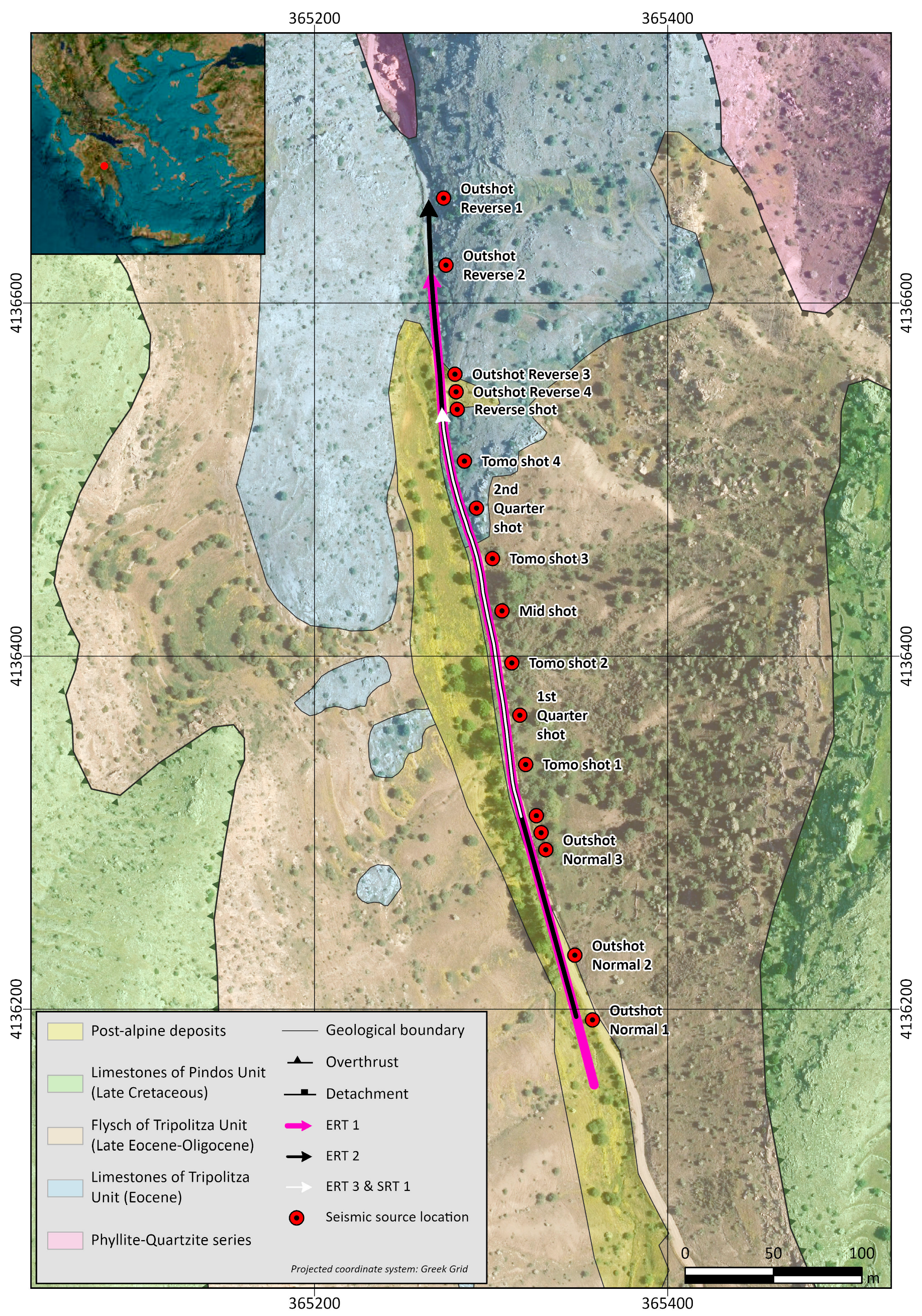
2.1. The First Study Area Kleisoura Valley, Ano Doliana

The first study area of Kleisoura Valley is primarily composed of Alpine formations that belong to three distinct geotectonic units of the Outer Hellenides. These units have been tectonically juxtaposed during the Alpine orogenetic cycle, involving processes associated with the initial stage of subduction and the late-orogenetic extensional stage.

For the needs of the present study, a detailed geological mapping at a scale of 1:7500 was carried out at the area where the near-surface geophysical survey was to be applied. In this way, we managed to identify the geological environment and surface structure of the study area and collect all the necessary information to evaluate the geophysical results. In Figure 1, the detailed geological map constructed for the study area is presented, where the location to which the geophysical survey was applied is noted by the red mark.

The study area includes the following Alpine units from bottom to top: the high-pressure metamorphosed Phyllite–Quartzite Unit, the very-low grade to non-metamorphosed neritic Tripolitza Unit and the uppermost pelagic Pindos Unit.

The lower unit is the Phyllite–Quartzite series of the Permo–Triassic age [27], which mainly consists of schists alternating with quartzites, metapelites and phyllites (Figure 2f). This series is characterized by abrupt changes in lithological facies both laterally and vertically. The main petrographic types in this series include greenschists with residual glaucophane and paragonite; schists with chloritoid and glaucophane; chloritic–paragonitic-muscovitic schists with garnet; mica–quartzites with hematite, ilmenite and tourmaline and muscovitic–quartzose phyllites with chloritoid. According to the existing mineralogical paragenesis (presence or absence of Na-amphibole) and due to the wide variety of petrographic types, the Phyllite–Quartzite series reflect a broad range of metamorphic conditions (T = 280–480 °C/P = 2–10 kb), corresponding to the blueschist and subsequent greenschist metamorphism facies [28].

The Phyllite–Quartzite series are tectonically overlain by the Tripolitza Unit, which is the lowest non-metamorphic unit observed in the study area, mainly comprising two formations: (a) an Oligocene flysch (Figure 2b), which is characterized by alternating fine-grained thin-bedded brownish sandstones, thin interbeds of pelites and sparse limestones lenses or interbeds, (b) massive- to thick-bedded and occasionally medium-bedded, grey–black, often bituminous and intensely karstic limestones and dolomites of Paleocene–late Eocene age (Figure 2a,d). In many cases, the transition from the Eocene limestones to the flysch is either gradual, marked by a few meters thick light-colored marly limestones (Figure 2a,c), or abrupt through high-angle faults (Figure 2d). It should be noted that several isolated Tripolitza limestones were observed, west of the provincial road, within the flysch of the same unit (Figure 2a). In these locations, the limestones appear to be folded and, in most cases, are bounded at their contact with the flysch by faults. Moreover, along the provincial road, an abrupt transition from the limestones to the flysch of the Tripolitza Unit was observed, characterized by the presence of thick breccia (non-cohesive to cohesive cataclasites) at the structural top of the limestones (Figure 2e).

The structurally highest unit of the region is the Pindos Unit (or Pindos nappe). The Pindos nappe primarily occupies the highest topographic regions, both west and east, along the central axis of the study area. The study area includes formations of the upper part of the stratigraphic column (e.g., the “Arcadian nappe”) [28], primarily pelagic thin-bedded biomicritic Cretaceous limestones (Figure 2a), alternating with thin chert layers and nodules and thin red to yellow pelitic layers. For the most part, the Pindos limestones are seen overlying the Tripolitza flysch, but in the southern part, they overlie the Phyllite–Quartzite series.

The post-alpine sediments are seen north of the study area and include polymict Pliocene conglomerates featuring clasts originating from all the units (including metamorphic rocks of the Phyllite–Quartzite series). Moreover, Quaternary river deposits are present, mainly found along the Kleisoura Valley stream and alluvial deposits of considerable thickness resulting from in situ weathering.

The thrusting of the Pindos Unit on the Tripolitza Unit took place during the Middle Eocene to Oligocene when the Tripolitza Unit was accreted in the overriding plate. Subsequently, this was followed by a synorogenic exhumation stage in the subduction channel and later by an extensional late-orogenic stage. Eventually, the metamorphosed Phyllite–Quartzite series were exhumed to upper crustal levels through a crustal-scale detachment system.

The detachment is exposed at the northern part of Kleisoura Valley, where the Tripolitza flysch and limestone are juxtaposed through a low-angle normal fault (dip ~10–20°), generally dipping towards the south. Conversely, in the southern part, the detachment fault presents a similar low-angle geometry (10–20°) but dips generally towards the north. This change in dip direction is attributed to later neotectonic high-angle normal faults that crosscut all the previous compressional and extensional structures.

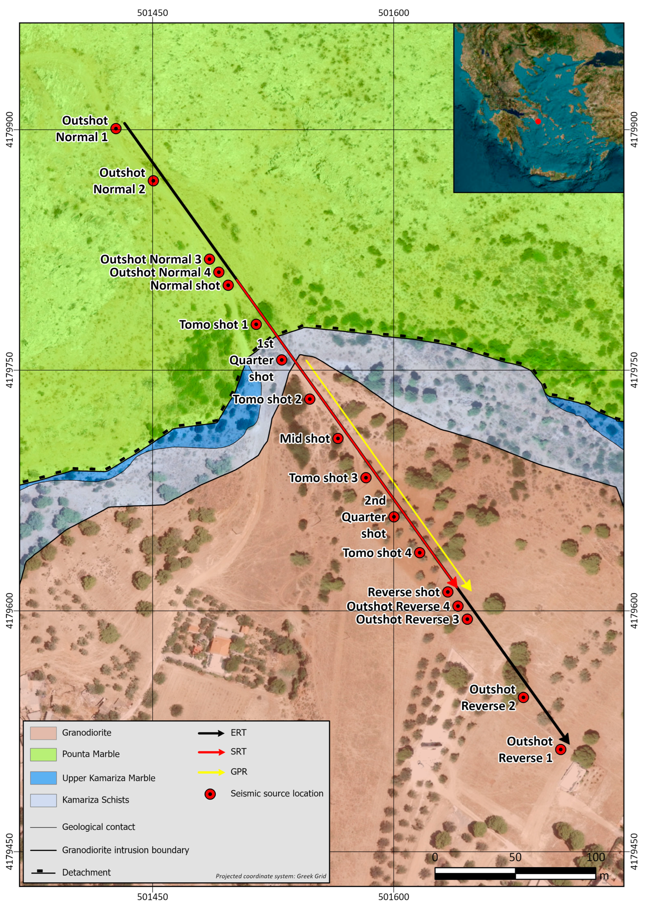
2.2. The Second Study Area “Plaka”

In Figure 3, the detailed geological map of the wider study area is presented, modified after [29], where the location to which the geophysical survey was applied is noted by the red mark.

Lavreotiki (south Attica) is located in the northwestern part of the Attic–Cycladic crystalline complex, and its structure is primarily controlled by a significant detachment fault with a top-to-SW sense of shear associated with the West Cycladic Detachment System [30,31]. The footwall of this detachment system includes formations of the Kamariza Unit, while the hanging wall is characterized by a complex structure that encompasses the metamorphic Lavrion Unit, the non-metamorphic Berzekos Unit and scattered occurrences of Neogene sediments. Moreover, the metamorphic units have been intruded by late Miocene magmatic bodies.

The Kamariza Unit is the structurally lowermost unit of Attica comprising three formations: the generally coarse-grained white Lower Kamariza Marble, the lithologically heterogeneous brownish calcareous Kamariza Schists (Figure 4g) and the white to blue–gray, ultra-mylonitic Upper Kamariza Marble (Figure 4f), with its upper boundary identified as the surface of the detachment fault (Figure 4a) [30,32,33]. Due to contact metamorphism, the Kamariza schists have become hornfels within a few hundred meters radius around the primary granodioritic intrusion [34].

The Lavrion Unit of the Mesozoic age is tectonically overlying the Kamariza Unit and constitutes the intermediate tectonic unit. It comprises from bottom to top the Triassic-Jurassic Pounta Marble (Figure 4e), the Lavrion schists and the Mavrovouni Marble [30]. The Lavrion Unit is characterized by Eocene age blueschist-facies metamorphism, followed by greenschist metamorphism during the Oligocene.

Finally, the uppermost unit is the non-metamorphic Berzekos Unit, which consists of radiolarites, sandstones and cherts and is rich in late Jurassic-early Cretaceous silicate fossils. On top of these formations, the late Cretaceous rudist-bearing limestones have been deposited unconformably. In most areas, these limestones have been infiltrated by hydrothermal fluids and have undergone ankeritization [34,35].

The Neogene continental deposits primarily consist of marls, siltstones and conglomerates, with clasts originating from the surrounding non-metamorphic units [34,35]. However, these deposits are not observed in the study area.

The magmatic intrusions include the main Plaka granodiorite with limited surface exposure, intruded within the Kamariza Unit. This intrusion is associated with contact metamorphism and sulfide mineralization [34]. Numerous small-scale intrusions with compositions ranging from dacitic to granodioritic have also been observed in the area [34,35,36,37]. The main granodiorite intrusion locally exhibits intense weathering, intensified by hydrothermal fluid circulation (Figure 4d), resulting in zones of varying mechanical and geophysical properties [29].

3. Methodology

To investigate the geologically complex subsurface structure of the two study areas, we employed a multidisciplinary, near-surface geophysical approach, utilizing the electrical resistivity tomography (ERT), seismic refraction tomography (SRT) and ground penetrating radar (GPR) techniques. More specifically, the ERT and the SRT techniques were applied to both study areas (Figure 5), while the GPR technique was used exclusively in the study area of Plaka. Furthermore, all the geophysical measurements were topographically corrected using a GNSS system.

In Figure 6 and Figure 7, the acquisition layout of the geophysical techniques applied in the first and second study areas is presented, correspondingly.

3.1. Electrical Resistivity Tomography

3.1.1. Data Acquisition

Across the first study area of Kleisoura Valley, Ano Doliana, two ERT profiles of 470 m (ERT 1 and ERT 2) and one of 235 m (ERT 3) were conducted, using 48 electrodes with a spacing of 10 m and 5 m, correspondingly (Figure 6). The two long profiles were executed in the same direction, with the ERT 2 profile shifted 40 m towards the north, resulting in a combined profile of 510 m total length. The short profile was designed to coincide with the center of the ERT 2 section. The application of the ERT 3 profile, with the smaller electrode spacing (5 m), aimed to increase the resolution of the technique in this intermediate part of the profile. This is expected to improve the delineation of the abrupt surface transition from the flysch to the limestones of Tripolitza Unit, verified by the presence of the tectonic breccia in this specific area.

Regarding the second study area of Plaka, two ERT sections of 470 m and 475 m were acquired (Figure 7), with 48 electrodes of 10 m and 5 m spacing, respectively, resulting in a joined ERT profile. The roll-along technique was implemented in two consecutive phases to cover the same profile length for the 5 m spacing section.

All the ERT measurements were acquired using the Wenner, Wenner–Schlumberger and Dipole–Dipole electrode configurations due to their different sensitivity regarding the way of the subsurface distribution of the electrical resistivity. Using the Electre Pro software V02.09.01, the sequences for the different electrode configurations were created for each ERT profile according to its geometrical characteristics. Subsequently, the sequences were imported to the Syscal Pro switch 48 (Iris Instruments, Orleans, France) resistivity meter to begin the automated data acquisition process. Moreover, a real-time generation of the apparent resistivity pseudosection was established using the FieldView software V02.00.02 to inspect the measurement sequence in the field directly.

3.1.2. Processing

The geoelectrical data were processed using the Res2DInv software v.4.9.11 by Geotomo [5]. Before the main processing, quality control of the data was performed, which included the extermination of noisy and inconsistent points (bad points). For the solution of the inverse problem, the smoothness-constrained least-squares method was applied, which is a modification of the Gauss–Newton least-squares equation [38], while the finite element method [39] was implemented for forward model calculation.

Depending on how the electrical resistivity of the subsurface varies, two different optimization methods are provided by the software. In the case where the electrical resistivity varies in a smooth and gradual manner, the l2 norm smoothness-constrained optimization method is proposed [40]. Conversely, when the electrical resistivity distribution is characterized by sharp and strong lateral variations, the l1 norm smoothness-constrained optimization method is recommended [41,42,43].

The subsurface structure of the first study area is expected to be characterized by steep transitions between geological formations, both laterally and vertically: laterally, due to the abrupt transition from the flysch to the limestone formations of Tripolitza Unit, and vertically, due to the expected existence of the Phyllite–Quartzite Unit, underlying the flysch and limestone, through the detachment fault. For the above reasons, the l1 norm smoothness-constrained optimization method (robust data constraint) was selected for the inversion of the geoelectrical data of the first study area. On the other hand, a more gradual subsurface resistivity distribution was expected due to the irregular shape of the granodiorite intrusion and the contact metamorphism of the Kamariza Schists in the second study area of Plaka. Therefore, the l2 norm smoothness-constrained optimization method (standard data constraint) was considered the most adequate for the calculation of the model parameters in this area.

Every ERT profile was processed separately for each of the three different electrode configurations applied. With this procedure, a total of nine and six different subsurface resistivity distribution models were generated for the first and second study areas respectively. The geoelectrical data obtained with the same electrode configuration were integrated into a unified clustered dataset, resulting in three ERT profiles (one for each electrode configuration) for each study area. Moreover, a combination of the datasets acquired with the three different electrode configurations across the same profiles was performed, but the final models were not geologically plausible. The most representative ERT section for each study area was selected taking into consideration the data quality and RMS or absolute percentage error between the observed and calculated resistivities, as well as the overall characteristics of the subsurface resistivity distribution.

3.2. Seismic Refraction Tomography

3.2.1. Data Acquisition

In both study areas, the recording of the P-wave first arrival times was carried out along a 235 m seismic line, using 48 geophones of 10 Hz natural frequency, with 5 m spacing. The Geometrics, San Jose, U.S.A., StrataView seismograph was used to record arrival times, to which the seismic receivers were connected via two multicore cables. The total recording time was 512 ms and a sampling window of 0.250 ms was used for signal digitization. Seismic waves were recorded from seventeen shot-points (Figure 6 and Figure 7), including four outshots on both ends of the seismic line, and nine shot-points in between the active spread with a 30 m shot interval.

The accessibility of the first study area (Kleisoura Valley, Ano Doliana) and the fact that it was located outside a residential area, allowed us to test several types of seismic sources, including three impact seismic sources and two explosive seismic sources. The impact seismic sources were two seismic sledgehammers of 3.5 kg and 6.5 kg and an accelerated weight drop (Geodevice, Calgary, Canada, AWD-33PS model) with 20 kg hammer weight. Subsequently, the electric seismic detonator and buffalo gun were used as explosive seismic sources.

In the second study area of Plaka, only the 6.5 kg seismic sledgehammer and the 20 kg AWD-33PS seismic source were feasible to use, with limitations. Since this area was located near a residential area, the use of explosive sources was prohibited.

3.2.2. Processing

Seismic data were processed using different modules of the Seismic Pro software v10.0 (Geogiga tech. Corp., Calgary, Canada) in three (3) main processing steps:

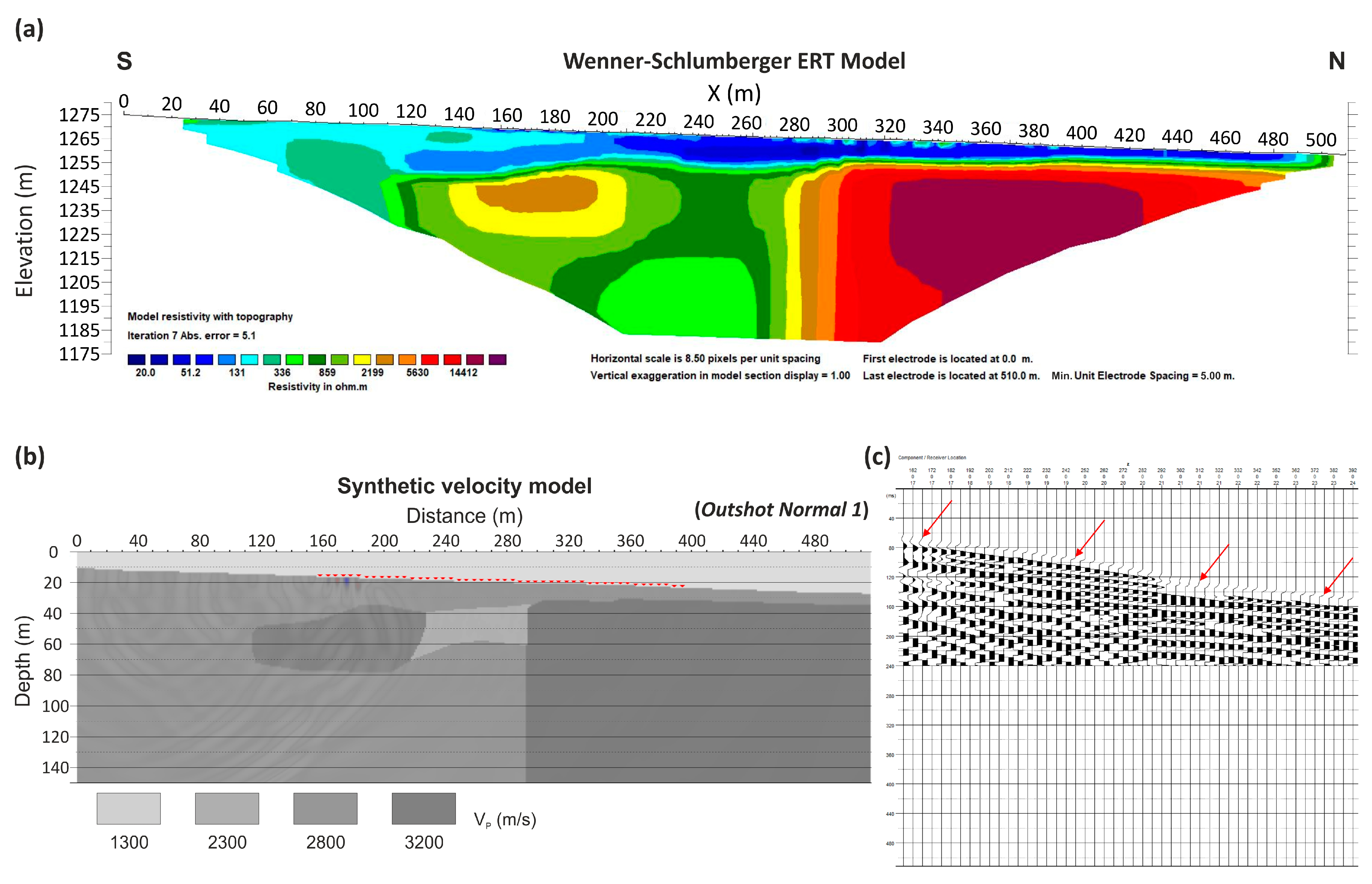
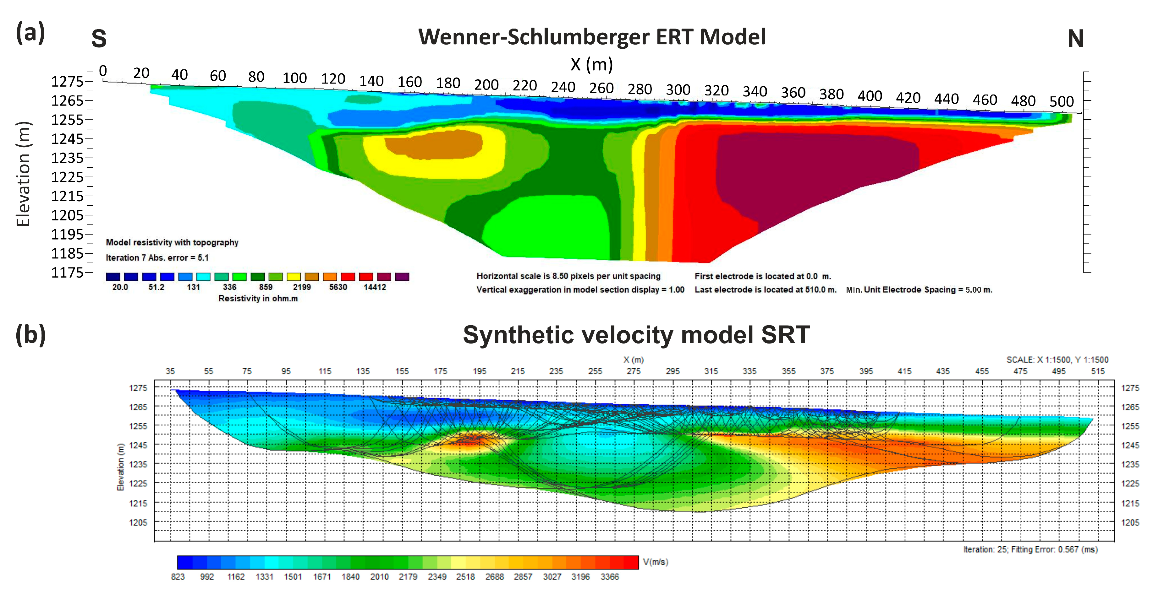
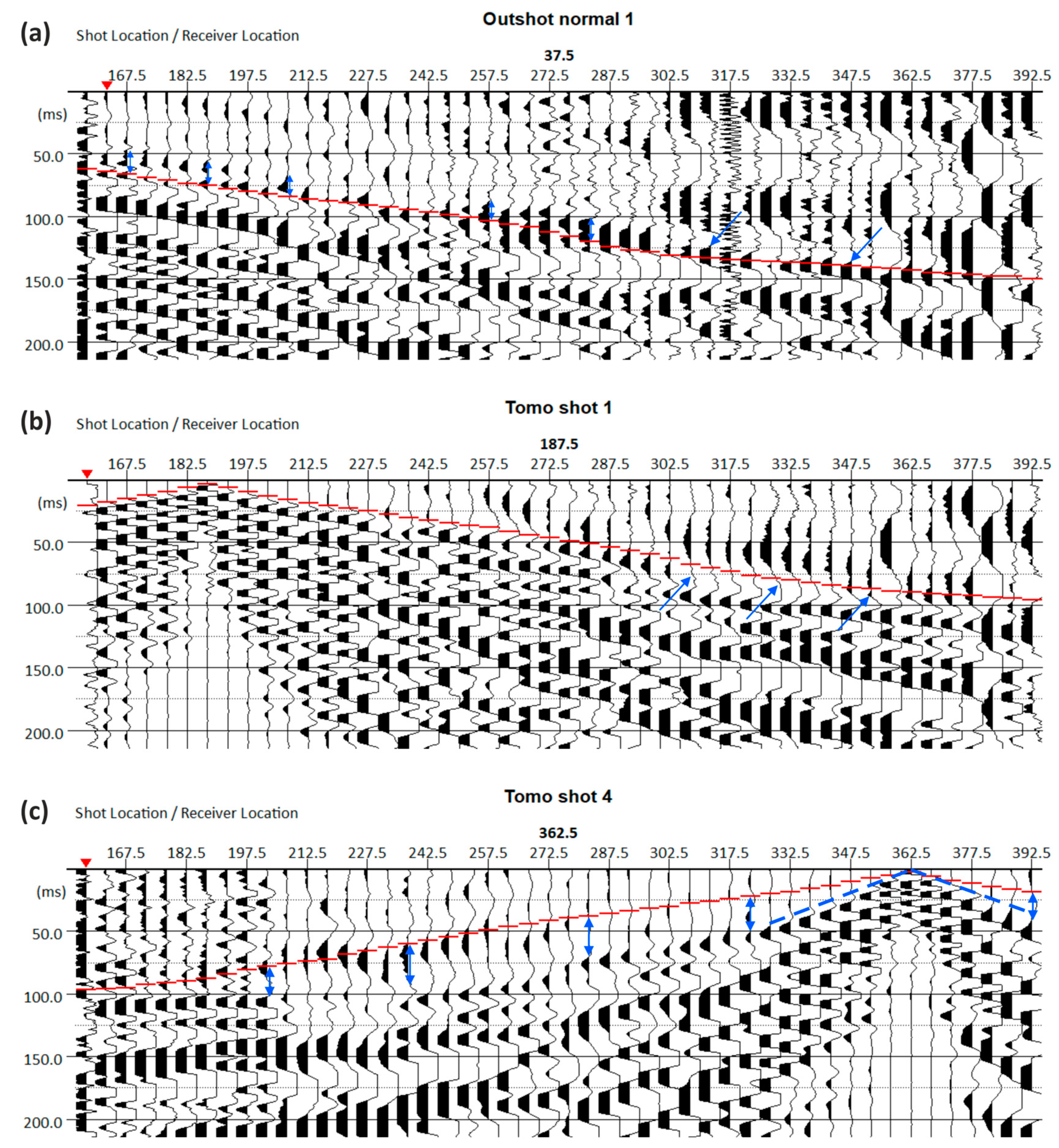
• Creation of synthetic seismic data (2D forward modeling) to determine the extent to which the SRT technique can provide a velocity model that best represents the complex subsurface structure characterizing the two study areas. Furthermore, by comparing the synthetic seismic records with the field seismic records, it was possible to attribute certain characteristics observed in the records to specific subsurface structures.
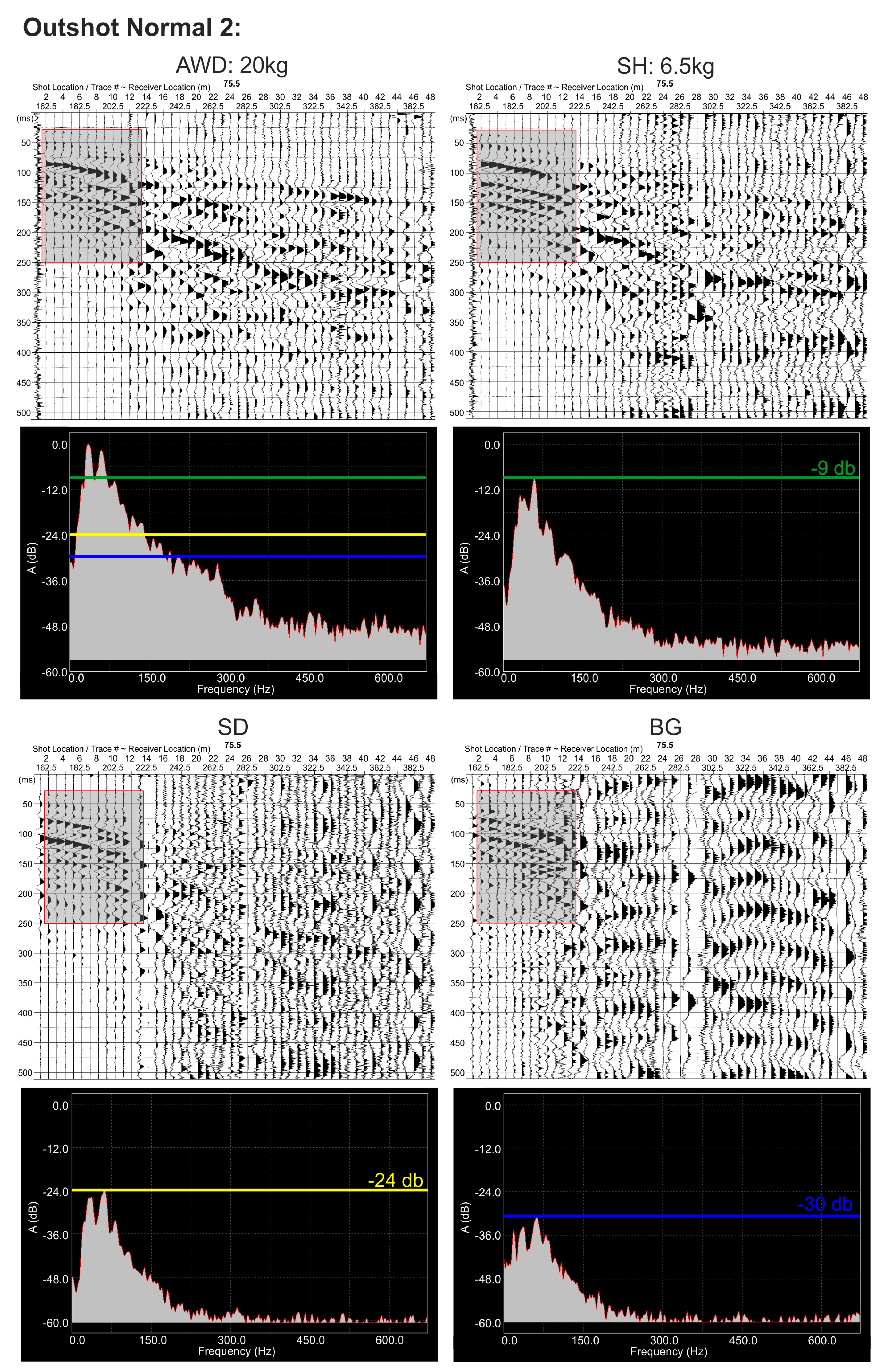
• Analysis and comparison of the seismic records acquired from the five different seismic sources to determine the type of seismic source that performed best in the specific geo-environment, providing the seismic records characterized by the highest S/N ratio.
• First brake picking and inversion of the seismic data to calculate the subsurface velocity models in the two study areas.

The creation of the synthetic seismic records was conducted using the Modeling 2D module, which incorporates the shortest path method [44] for forward modeling calculation. Seismic rays’ trajectories and corresponding travel times were calculated based on a predefined velocity model that was created taking into account the surface geological observations and the results of the ERT technique (Figure 8), given that it was the only available information regarding the subsurface structure for both study areas. Moreover, an initial subsurface velocity estimation was conducted by incorporating the intercept-time method in the field seismic records.

In general, resistive formations were modeled as compacted formations, characterized by high seismic velocity values, while conductive formations were modeled as less compacted formations or unconsolidated sediments, with lower seismic velocity values. An exception was the Kamariza Schists in the second study area, which were characterized by low resistivity and high-velocity values.

Seventeen synthetic seismic records were created for both study areas, simulating the data acquisition layout incorporated in the field. Subsequently, the first breaks were manually picked on the synthetic datasets, and the synthetic travel times were then inverted using the smoothing-constrained regularized inversion approach of the DW tomo module. During the inversion process, several parameters were tested regarding the min. and max. velocities, the allowable percentage of change in the velocity per iteration, the horizontal and vertical smoothing lengths as well as the smoothing weighting factor. Afterward, synthetic travel times obtained from the synthetic seismic records were superimposed on the field seismic records of the same shot location to determine whether the synthetic travel times were consistent with the actual travel times. This processing sequence was repeated many times by altering the initial velocity model parameters and inversion settings, until a geologically plausible velocity model was obtained, similar to the synthetic one, with minor deviations between the modeled and observed first break travel times.

The selection of the appropriate type of seismic source is crucial, as the characteristics of each source affect the quality of the data, the maximum depth of investigation and the maximum resolution that can be achieved [45,46]. According to several researchers [47,48], selecting the appropriate type of seismic source should be based on the following criteria: maximum depth of investigation, appropriate frequency content, S/N characteristics, investigation field limitations, availability and operation cost. In general, the most critical factors for selecting the proper seismic source type for seismic data acquisition are the energy and frequency content of the generated signal [46,49,50,51], as well as the repeatability of the source [52,53]. The signal characteristics emitted by a source are affected by many factors. The way the data are acquired (single or consecutive records), as well as the recording and processing parameters, are some factors that affect the signal’s characteristics. In addition, the surface and subsurface conditions in the area where the survey is carried out greatly influence the amplitude and frequency content of all types of recorded waves.

Seismic sources signal analysis and comparison were carried out only for the first study area, given that this area allowed us to utilize all five seismic sources for the data acquisition. Comparisons were made between the seismic records acquired at each shot-point from the five seismic sources used. Both the recording and processing parameters were kept constant at each location. The amplitude spectral content diagrams were constructed for all seismic records by applying the fast Fourier transform. For each seismic record, a specific time window was selected for the analysis to be performed to analyze the part of the record characterized by the highest quality signal. The amplitude spectra of the seismic records are represented relative to the reference level (0 dB), representing the maximum recorded amplitude. Negative dB values indicate whether the amplitude of different frequencies is smaller than the reference level. In addition, the amplitude spectra diagrams of the different seismic sources, constructed at each shot-point, are presented normalized to the one characterized by the maximum energy.

The field seismic records were processed using the DW tomo module. The first processing step was creating a group file list, which included the seventeen seismic records characterized by the best S/N ratio, with the clearest first breaks, thus facilitating the management and processing of the data. In both study areas, all the seismic records acquired with the AWD-33 PS seismic source were used, as well as the seismic records obtained with the 6.5 kg sledgehammer, but only in the case of the second study area. At this step, the geometrical characteristics and the topography of the seismic developments were also defined. Moreover, low-pass Butterworth filters with a cut-off frequency of 200 Hz and a slope of 12 db/oct, as well as adjustment of the signal gain, were applied in order to remove the high-frequency noise and highlight the first breaks in the seismic records respectively.

Manual first break picking was efficiently accomplished in fourteen (14) and in ten (10) out of the seventeen (17) acquired seismic records for the first and second study areas, correspondingly. The high vegetation, the possible existence of underground mining galleries, the anthropogenic deposits (mining debris) of the old mines excavations located at the central part of the seismic section and the difficulty of carrying and utilizing the AWD-33PS seismic source in the outshot positions resulted in the unsuccessful recording of the first arrivals in the second study area and thus a significant loss of information. Afterward, a primary processing was carried out by applying the intercept-time method in order to calculate a gradient initial velocity model. In the case of the first study area, P-wave velocity was calculated equal to 1070 m/s near the surface, gradually increasing to 2435 m/s until the depth of 17.3 m and further increasing to 4240 m/s until the depth of 70 m. Conversely, the initial velocity model calculated for the second study area was characterized by 1360 m/s surface velocity, gradually increasing to 2550 m/s until the depth of 22 m and further increasing to 5840 m/s until the depth of 60 m.

For the calculation of the subsurface P-wave velocity models, the smoothing-constrained regularized inversion approach was applied to invert the seismic data. For model smoothing, 15 m and 6.25 m horizontal and vertical smoothing lengths were set, respectively, while for the inversion limitation, a maximum change of 60% in average velocity per iteration was allowed. A total of 30 iterations were defined for the inversion process, with the possibility to select the desired result from any iteration cycle. The shortest path method [44] was incorporated for the forward modeling solution, with horizontal and vertical model cell dimensions equal to 2.5 × 1.25 m, corresponding to the ½ and ¼ of the geophone spacing, respectively.

3.3. Ground Penetrating Radar

The broader area of Plaka was submitted in extensive mining campaigns from the Classical period until the late 20th century. Thus, several mining galleries are present in the entire region, including the second study area. Due to the possible existence of such galleries throughout the selected geophysical line, the GPR method was implemented in an effort to locate any possible underground mining corridors [54].

3.3.1. Data Acquisition

GPR data were acquired along a 177 m line, starting from the 14th geophone up to the end of the seismic line (Figure 7). A bistatic 100 MHz shielded antenna (Noggin 100,Sensors and Software, Mississauga, Canada) was used to achieve a satisfactory investigation depth (~15 m), while the pulse transmission step (5 cm trace interval) was controlled by an odometer wheel. In each step, several E/M pulses were stacked to improve the S/N ratio by incorporating a feature of the GPR system, which automatically controls the number of stacks depending on the conductivity of the medium.

3.3.2. Processing

GPR data were processed using the Ekko Project 6 software by applying a standard filtering procedure including Dewow, background removal, bandpass filter, SEC2 gain and f-k migration using the hyperbola fitting method.

4. Results and Discussion

4.1. Forward Modeling

In Figure 9, the seismic tomogram calculated after the inversion of the synthetic traveltimes is presented with respect to the ERT results, based on which the initial subsurface velocity model was created for the first study area (Kleisoura Valley, Ano Doliana). It is evident that all the structures simulated by the construction of the synthetic subsurface velocity model are highlighted. More specifically, both the high resistivity regions, simulated as high-velocity formations, are adumbrated by the SRT technique in a 165–215 m distance and at the second half of the profile. Moreover, the subvertical electrical discontinuity simulated as a strong lateral velocity variation is delineated at a 300 m distance, as well as the low-velocity region in the middle part of the profile, with the characteristic U-shaped form of the iso-velocity curves. Therefore, we conclude that the SRT technique could render, to a fairly satisfactory degree, the complex subsurface structure considered for this case.

In Figure 10, we present three (3) indicative examples of overlaying the synthetic first arrival times onto the field seismic records acquired with the AWD-33PS seismic source at three (3) different shot locations. The red symbols mark the synthetic first arrivals, while the position of the true first arrivals or their divergence from the synthetic ones is indicated with the blue arrows.

Regarding the outshot normal 1 shot-point (Figure 10a), located at 120 m offset, a slight divergence of 15 ms on average is observed between the synthetic and true first arrivals. However, the general distribution of the synthetic first arrivals is consistent with that of the true ones. Furthermore, the simulation of the low-velocity region in between the high-velocity formations proves to be reasonable, as indicated by the increase in the slope of both the synthetic and true refracted arrival times at 257.5–297.5 m distance.

Similarly, a minimal divergence of less than 5 ms is observed in the case of the tomo shot 1 shot-point (Figure 10b). In general, the position of the synthetic first arrivals is identical to the position of the true arrivals in the overall record. Small divergencies are observed in a few seismic traces after the 300 m distance, where the subvertical electrical discontinuity was investigated.

Finally, in the case where the shot-point is located at distances greater than 300 m (Figure 10c), large divergencies are observed between the synthetic and true travel times, on both the direct and refracted arrivals. The higher slope of the true direct arrivals indicates a lower seismic velocity at shallow depths for the seismic formation located at distances greater than 300 m. While in the two previous cases, the synthetic and true refracted arrivals were almost identical for the same traces, the divergence observed on the direct arrivals indicates a vertical gradient in the seismic velocity of this formation.

In this case, the large divergencies observed between the direct and refracted arrivals are attributed to the strong lateral and vertical heterogeneity that characterizes the subsurface structure of the study area, which was not accounted for in the initial velocity model constructed for modeling. On the contrary, the initial velocity model was simulated by a subsurface structure characterized by the presence of discrete, homogeneous and uniform seismic formations.

4.2. Source Comparsion

In Figure 11, an indicative example of the seismic records and their corresponding amplitude spectra plots are presented for the outshot normal 2 shot-point (82 m offset) acquired with the AWD-33PS (AWD 20 kg), 6.5 kg sledgehammer (SH 6.5 kg), seismic detonator (SD) and buffalo gun (BG) seismic sources. The amplitude spectrum of the 3.5 kg sledgehammer (sh 3.5 kg) was very similar to the 6.5 kg sledgehammer (SH 6.5 kg) source; therefore, it is not presented in this case.

Regarding the seismic records acquired with the explosive seismic sources from the 13th seismic trace onwards, i.e., at distances greater than 142 m from the shot-point, high-frequency noise predominates. As for the impact seismic sources records, these were acquired by four and six vertical stackings for the AWD 20 kg and SH 6.5 kg sources, respectively. In the seismic record of the SH 6.5 kg source, there is a lot of high-frequency noise contamination from the 19th trace to the end of the record, which makes it difficult to identify the P-wave arrival times. Significant improvement is observed in the AWD 20 kg seismic record, where P-wave arrival times are distinct and noise levels are low, even in the most distant seismic traces.

For signal analysis, the time window of 28–250 ms from the 2nd to the 13th seismic trace (Figure 11—grey shaded box with red outline) was chosen. Within the selected window, P-wave refracted arrivals are discerned at 37 ms and 60 ms for the 2nd and 13th seismic traces, respectively, while after 75 ms, surface waves dominate. All the amplitude spectra plots are presented normalized to the AWD 20 kg source plot, which is characterized by the highest energy amplitudes. The maximum energy amplitudes of the BG, SD and SH 6.5 kg sources are marked by the blue, yellow and green horizontal lines, correspondingly, and they are concentrated in a frequency band near 60 Hz. In the case of the AWD 20 kg source, the corresponding amplitude is increased by 30, 24 and 9 dB in comparison with the BG, SD and SH 6.5 kg sources, respectively.

Most of the body and surface wave energy is concentrated within a frequency bandwidth of 10–150 Hz for the selected time window. Furthermore, there is much less damping of the high-frequency wave amplitude in the case of the AWD 20 kg source compared to the others. This variation is due to the higher energy released by the AWD 20 kg source, along with the fact that the damping of the seismic energy is proportional to the frequency and propagation distance of the seismic waves.

4.3. Field Data Results of the First Study Area Kleisoura Valley, Ano Doliana

The results of all the geophysical techniques applied in the first study area, along with their representative geological profile, created after the combined evaluation of the results, are presented in Figure 12. The Wenner–Schlumberger ERT profile was considered the most representative of the subsurface structure. Due to the wide range of resistivity values, the logarithmic scale was chosen to visualize the data distribution. The SRT profile was finalized after the 22nd iteration of the inversion process, achieving a divergence of less than 3 ms between the calculated and observed first arrivals.

Regarding the subsurface resistivity distribution (Figure 12a), the lower resistivity values (<50 Ohm·m) appear to be constrained near the surface, between a 190–485 m distance down to a depth of 3–12 m. Very characteristic is the presence of a sharp, subvertical electrical discontinuity, located at a 300 m distance and depths greater than 10 m. This discontinuity separates two areas characterized by a strong contrast between their resistivity values, emphasizing the lateral heterogeneity of this study area. At distances greater than 300 m (north of the electrical discontinuity) to the end of the profile, underlying the surface conductive zone, a highly resistive formation is identified, with resistivity values greater than 5600 Ohm·m. From the beginning of the ERT profile, up to 300 m distance (south of the electrical discontinuity) and underlying the surface conductive zone, a less resistive region is investigated, with resistivity values lower than 3500 Ohm·m. A further distinction can be made within this region concerning the electrical resistivity distribution. Between a 135–210 m distance and for an average depth of 15–45 m, a resistive formation is identified, characterized by resistivity values ranging from 1300–3500 Ohm·m. In the remaining part of the profile, the subsurface model is characterized as relatively resistive, with resistivity values between 100–1000 Ohm·m.

In Figure 12b, the final P-wave tomographic model obtained after the 22nd iteration of the inversion process, with a 3 ms RMS error, is presented. The subsurface velocity distribution is characterized by strong lateral variations and the presence of regions with high vertical gradients. Low P-wave velocity values of 800–1300 m/s are concentrated at the near-surface part of the profile, at distances greater than 180 m to the end of the profile. Between a 220–345 m distance, an arched shape of the iso-velocity curves is observed, resulting in a strong lateral variation in the 12–40 m depth range. From the start of the profile to a 180 m distance, higher P-wave velocity values are investigated (1700–3000 m/s), which underlies the abovementioned low-velocity values at greater distances. In particular, from the start of the profile to the 135 m distance, a high vertical velocity gradient is observed, where the V_P rapidly increases from 1700 m/s at the surface to 3000 m/s at the depth of 20 m. Between a 135–220 m distance, a high-velocity region is present until the average depth of 45 m, with V_P = 2400–3000 m/s. On the central part of the profile (265–335 m) and in the depth range of 40–65 m, a region characterized by V_P = 1900–2400 m/s is present, with the characteristic U-shaped form of the iso-velocity curves, resulting in a lateral velocity variation in respect with the adjacent regions at this depth. At distances, greater than 345 m to the end of the profile and a depth range of 10–65 m and 5–20 m, correspondingly, a wide variety of velocities is identified (1700–3000 m/s), characterized by a lower vertical velocity gradient in conjunction with the first part of the profile. Finally, a high-velocity (V_P > 3000 m/s) formation has been investigated throughout the whole profile length and at the greatest investigation depths. At the southern and northern parts of the profile, the top of this formation is present at 20 m depth, while towards the central part of the section, it is investigated in progressively greater depths, reaching the maximum value of 65 m at 315 m distance.

The final geological interpretation of the geophysical results is presented in Figure 12c, which was derived from the combined evaluation of the ERT and SRT techniques and taking into consideration the geological observations and data collected during the detailed geological mapping that was carried out in the area.

The location where the subvertical electrical discontinuity was investigated by the ERT technique is in agreement with the location where the abrupt lateral transmission from the flysch to the limestones of the Tripolitza Unit was observed. Moreover, the tectonic breccia at this location led to evaluating this discontinuity as a normal south-dipping fault, which brings these two geological formations into contact. Another indication supporting this interpretation is the strong lateral variation observed in the distribution of the seismic velocities in a 50 m width vertical zone symmetrically to the fault’s location. This zone is characterized by V_P values of 1200–2400 m/s, indicating the degradation of the mechanical properties of the subsurface formations in this region due to the fault’s impact. Furthermore, according to the SRT profile, the fault appears to develop down to 65 m depth, as at greater depths, a high-velocity (V_P > 3000 m/s) formation is observed, which does not seem to have been affected by the fault.

From a 190 m to 485 m distance, the low-resistivity (<50 Ohm·m) and low-velocity (800–1100 m/s) geophysical formation is interpreted as the incohesive soil sediments of the alluvial deposits. These deposits are characterized by a 12 m maximum thickness and overlie the fault zone at 300 m distance. The high conductivity of these deposits is due to the phreatic aquifer that develops within them, while the low-velocity values are attributed to the fact that they consist primarily of loose, non-cohesive soil materials, products of the weathering and erosion of the adjacent geological formations.

At distances greater than 300 m (north of the fault’s location), the high resistive formation (>5600 Ohm·m), which is also characterized by a wide variety of seismic velocities, V_P = 1300–3000 m/s, is geologically interpreted as the Tripolitza Unit Eocene limestones. This formation develops underlying the alluvial deposits, except for the last 25 m of the profile where it is exposed on the surface. The maximum thickness of this formation is located at 300 m distance where it reaches 55 m, while towards the end of the profile, it continuously decreases, reaching the minimum value of 20 m. According to field observations, the limestones appear to be highly karstified at this location, which justifies both the high resistivity values and lower seismic velocities that were investigated. Another factor that has significantly downgraded the formation’s seismic velocity (1300–1900 m/s) is the fault’s activity in a zone of 25 m width. The relatively intact part of the formation is observed at distances greater than 25 m from the fault’s location to the end of the profile and at depths greater than 30 m, where it is characterized by V_P = 2200–3000 m/s.

The deepest investigated seismic formation, characterized by high V_P values of 3000–4400 m/s, is interpreted as the bedrock of the study area, consisting of the metamorphic lithologies of the highly heterogeneous Phyllite–Quartzite formation. Quartzite is characterized by higher V_P values than phyllite, which justifies the lateral variations in the formation’s velocity. This formation was investigated near the surface at the beginning and the end of the profile, at depths greater than 20 m, while towards the central part of the profile (295–355 m), it is observed at depths greater than 65 m. This formation is in contact with all the overlying formations through the detachment fault, identified in the field at about 40 m northern to the end of the geophysical line.

The resistive formation (1300–3500 Ohm·m) investigated between a 135–210 m distance and at a 15–45 m average depth range, characterized also by high V_P values of 2400–3000 m/s, is interpreted as a local occurrence of Tripolitza Unit limestones. At this location, the limestones are characterized by higher seismic velocity and lower resistivity values than those north of the fault. This indicates that they have been affected to a much lesser extent by the karstification phenomenon, probably because they are surrounded by impermeable formations, which prevented the development of the karstification phenomenon.

The remaining part of the profile, characterized by the presence of a relatively resistive formation (100–1000 Ohm·m), with seismic velocities varying from 1200–3000 m/s, is interpreted as the flysch of the Tripolitza Unit. At distances greater than 185 m, the flysch is underlying the alluvial deposits, up to 300 m distance, where it comes into contact with the Tripolitza Unit limestones through the fault. Generally, the low-velocity values occur near the surface but with a high vertical velocity gradient. The lower velocity (1200–2200 m/s) and higher resistivity values (500–1000 Ohm·m) are observed near the fault’s location. The flysch is also a highly heterogeneous formation, consisting of sandstone and clay alternations, which justifies the lateral variation of both its resistivity and velocity values.

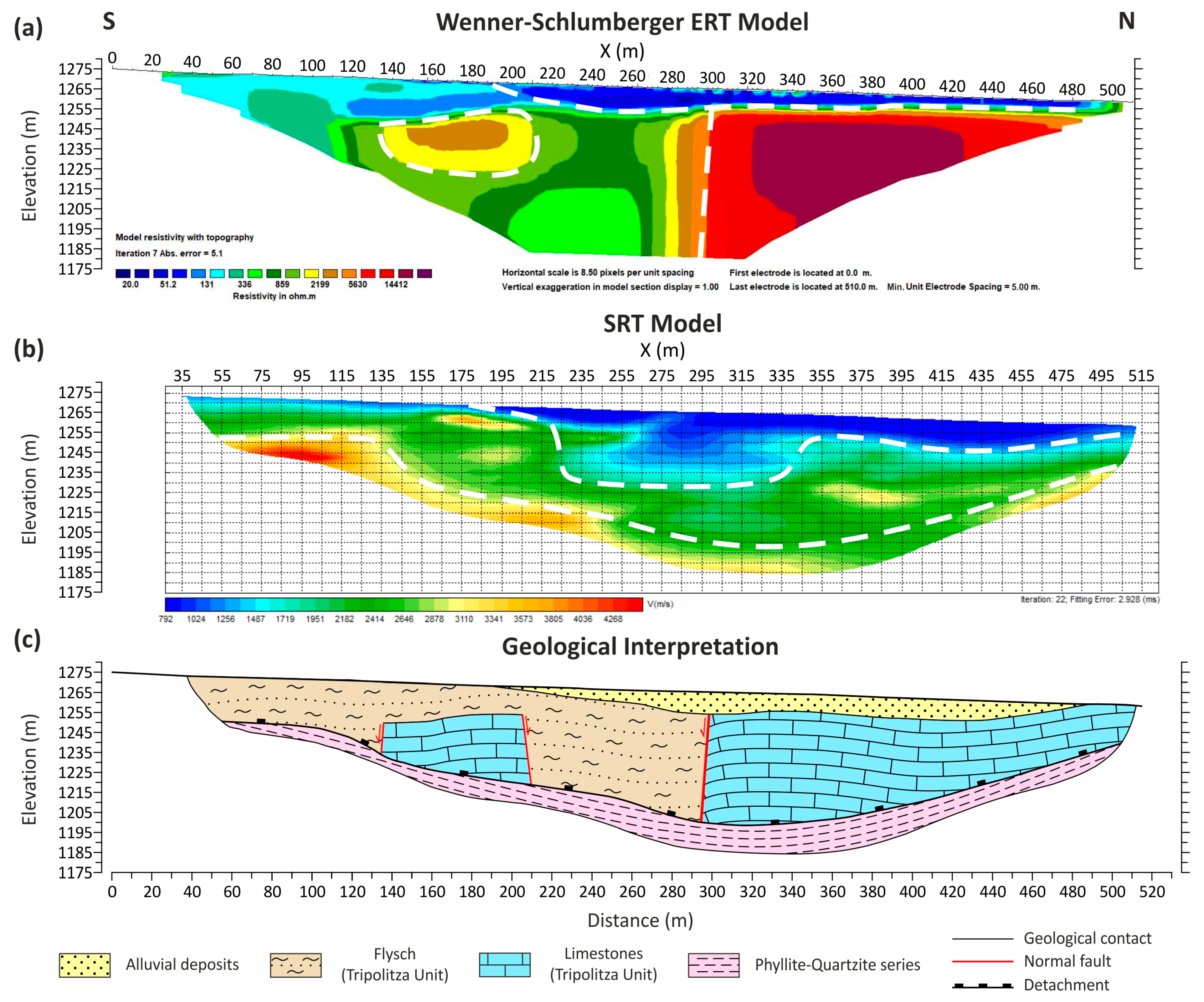
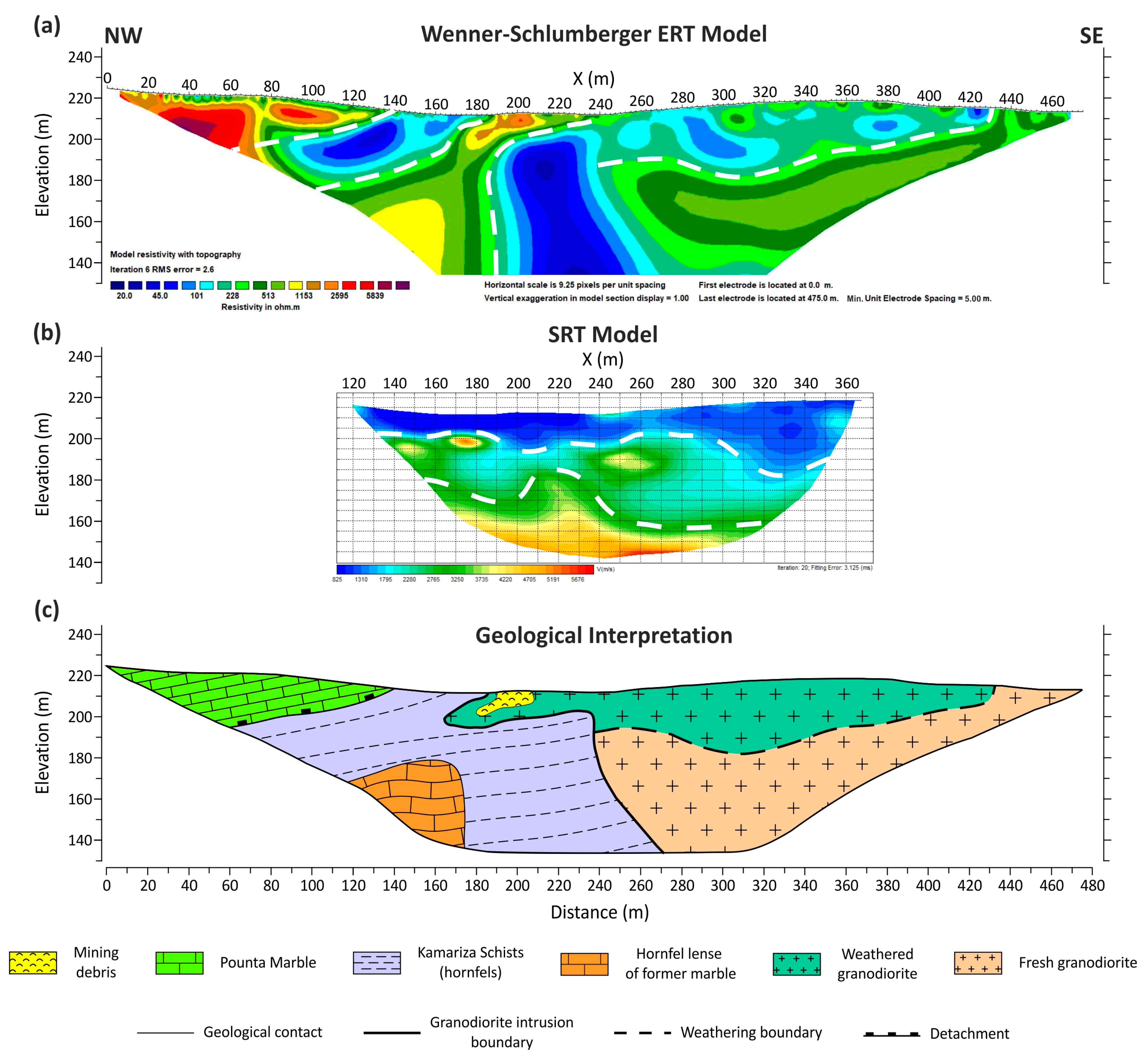
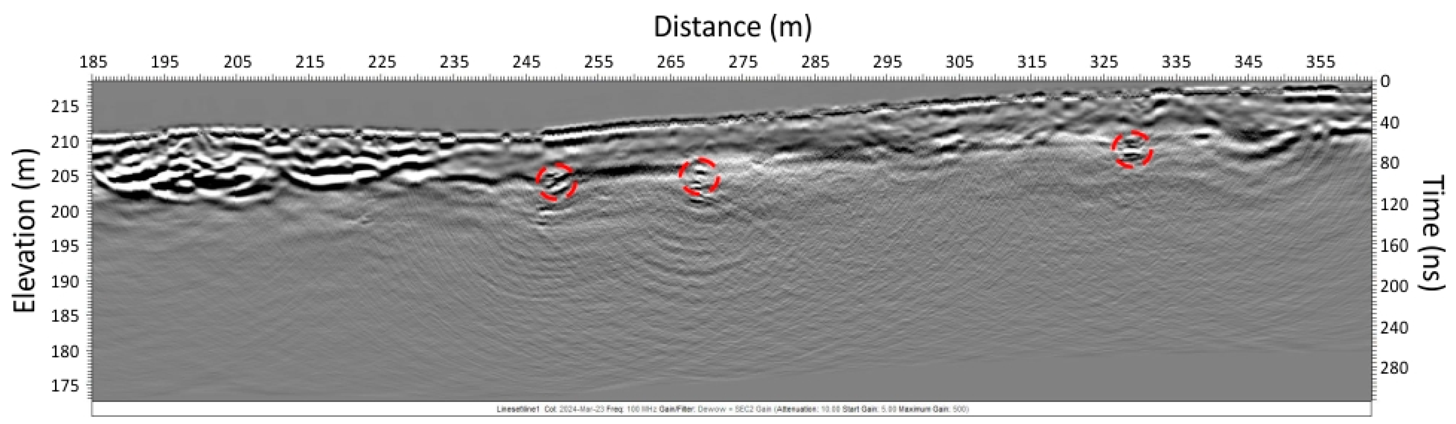
4.4. Field Data Results of the Second Study Area “Plaka”

The results of the ERT and SRT techniques applied along the geophysical line of the second study area, as well as their geological interpretation are presented in Figure 13. The ERT profile considered as the best representation of the subsurface structure, was the one obtained by the Wenner–Schlumberger dataset processing and is illustrated using a logarithmic scale for its resistivity distribution visualization. The subsurface velocity model was calculated after the completion of the 20th iteration of the inversion process, with a deviation between the calculated and observed arrival times of less than 3.2 ms.

In the NW part of the ERT profile (Figure 13a), a highly resistive (>1000 Ohm·m) formation is observed from the beginning to 140 m distance. The maximum investigated depth of this formation is 27 m, located at 62 m distance, while it seems to decrease towards the SE gradually. From a 90–185 m distance and underlying the aforementioned resistive formation, a conductive zone with resistivity values of 20–100 Ohm·m is delineated. At distances between 140–185 m, the zone develops close to the surface, and it is characterized by an average thickness of 22 m. A second conductive zone, with the same resistivity values, is identified at 190–240 m distance and at depths greater than 10 m. The second zone is characterized by an average width of 60 m and extends up to an 85 m depth, corresponding to the maximum investigation depth of the technique. These two conductive zones are separated by a resistive formation, with resistivity values ranging from 350–2500 Ohm·m. At distances less than 185 m, this formation underlies the first investigated conductive zone, while between a 185–240 m distance, it develops close to the ground surface. The high resistivity values (1200–2500 Ohm·m) of this formation are confined near the surface at 185–205 m distance, while the rest is characterized by lower resistivity values (350–1000 Ohm·m). At distances greater than 240 m to the end of the ERT profile, the subsurface resistivity values range from 45 to 800 Ohm·m. From the surface and up to an average depth of 35 m, lower resistivity values (45–200 Ohm·m) dominate, while at greater depths, higher resistivity values (250–800 Ohm·m) are observed.

Regarding the subsurface velocity distribution of the SRT profile (Figure 13b), the lower seismic velocities (800–1600 m/s) are constrained in the near-surface part of the section, where a slight increase in the velocities is observed at the second half of the profile. From 120–290 m distance, this low-velocity zone has an average thickness of 10 m, while at greater distances, an increase in the zone’s thickness occurs, reaching the maximum value of 35 m at a 330 m distance. Underlying, a second velocity zone is delineated, characterized by a wide range of seismic velocities (1800–4700 m/s) and thickness varying from 10–45 m. The majority of this zone is observed with seismic velocity ranging between 1800–2700 m/s. However, there are some local regions within which the highest seismic velocities of this zone are concentrated. They are located between 140–185 m and 240–270 m distance, in a depth range of 10–30 m and are characterized by high V_P values, ranging from 3700–4700 m/s. Finally, a third velocity zone characterized by the highest velocity values is investigated at the deepest part of the profile. In this zone, V_P values greater than 3000 m/s are observed, while seismic velocities of 5800 m/s are also present. This zone is located at depths greater than 30 m and 58 m, located at 155 m and 320 m distances, correspondingly, while between a 205–240 m distance, an updoming of the iso-velocity curves in this zone is observed.

The SRT profile of the second study area was significantly limited compared to the corresponding model of the first study area due to the unsuccessful recording and processing of the outshot seismic records. For that reason, the geological interpretation (Figure 13c) was mainly based on the ERT results, apart from the joint section of the two geophysical techniques based on their combined evaluation.

The highly resistive formation (>1000 Ohm·m) that develops close to the near-surface, at the NW part of the ERT profile, is evaluated as the Pounta Marble, which is consistent with the geological mapping of the area. According to surface geological observations, these marbles appear highly karstified in places, justifying the increased resistivity values. The maximum investigated thickness of this formation is 27 m, located at 62 m distance, gradually decreasing towards the SE up to 140 m distance.

The two conductive zones (20–100 Ohm·m) investigated by the ERT technique, as well as part of the relatively resistive zone (350–1000 Ohm·m), located at depths greater than 17 m, between the two conductive zones, are interpreted as the Kamariza Schists, which have been contact metamorphosed into hornfels. In several locations near the study area, surface occurrences of massive hornfels lenses of former marble have been observed within the Kamariza Schists (Figure 4c). These lenses may account for the increased resistivity values located between the two conductive zones. The first 10–15 m of the formation’s thickness are characterized by velocities of V_P = 800–1800 m/s, while at greater depths, a significant increase in the velocity values is observed, ranging from 2800–4800 m/s. The highest seismic velocity values are concentrated in a zone between a 205–240 m distance, at depths greater than 35 m. At distances less than 140 m, the Kamariza Schists underlies the Pounta Marble. The contact between these two formations is the detachment fault, which dips to the NW and is clearly delineated from the ERT profile (Figure 13a). According to geological observations, the Kamariza Schists are highly heterogeneous. Its mineralogical composition consists primarily of phyllosilicate minerals (mainly chlorite and white micas), with intense weathering and hydrothermal alteration; in other places, the carbonate minerals predominate. This heterogeneity accounts for the lateral variations observed in both the resistivity and seismic velocity investigated values.

The high resistivity (1150–3500 Ohm·m) and low velocity (800–1000 m/s) values investigated between 190–210 m distance, from the surface to the maximum depth of 7 m, are attributed to the presence of anthropogenic deposits, consisting by the excavation waste materials from the old mining activity. During the data acquisition campaign, these deposits were also observed in the field at this exact location (Figure 4b).

Considering the subsurface distribution of the resistivity and P-wave velocity values at the profile’s segment, located at distances greater than 170 m and overlying the Kamariza Schist formation, two different regions can be distinguished. The first one is located from the surface to an average depth of 12 m, between a 185–240 m distance, while from a 240–430 m distance, until the average depth of 25 m. Low-resistivity (50–350 Ohm·m) and low-velocity (800–1500 m/s) formations seem to dominate within this region. Geologically, it is interpreted as the Plaka granodiorite formation, which, according to our field observations, is strongly weathered and hydrothermally altered [29]. Some of the circular forms could represent woolsack weathering. The thickness of this weathering-affected layer appears to decrease towards the SE, e.g., away from the ravine that runs through the granodiorite. The second region is located underlying the first one, extending to the maximum investigation depth of the two geophysical techniques. Higher resistivity (400–770 Ohm·m) and higher velocity (2000–5500 m/s) values are observed within this region. These increased values can be justified by the presence of the Plaka granodiorite, which, in this case, has been affected to a much lesser extent by the weathering processes. In general, the P-wave velocities of this formation appear to increase with respect to depth, indicating a compact, fresh granodiorite existing at greater depths. According to the distribution of the resistivity values at distances greater than 430 m, this formation appears to develop close to the surface, which is consistent with the geological mapping and the observations carried out in the field.

In Figure 14, the processing results of the GPR line for the second study area are presented. The method highlights the possible existence of air voids (GPR signal velocity ~0.3 m/ns) marked as red dashed circles, at 62 m, 84 m and 144 m distances at a depth of approximately 7 m. These air voids are interpreted as possible old mining galleries in the area.

5. Conclusions

The multidisciplinary approach carried out across the two geologically complex investigation fields confirmed the advantages of the combined application and interpretation of the electrical resistivity tomography (ERT) and seismic refraction tomography (SRT) techniques. Beyond the technical assessment of optimum data acquisition and processing parameters for these geophysical techniques, this approach provided an initial understanding and connection between the surface geological observations with the near-surface geotectonic subsurface structure of the two study areas.

The present study demonstrated that the ERT technique is the primary technique for subsurface investigation in such complex geological environments. Compared to the SRT technique, it provides greater flexibility in the field, making it less time-consuming and more cost-effective. The ability to acquire measurements with different electrode configurations and to choose among various optimization methods regarding the inversion process allows researchers to adopt the best possible approach for the ERT investigation, depending on the expected variations in resistivity. Additionally, the ERT technique does not require an initial model input for data processing, making it an ideal primary methodology, prior to the design and application of the SRT technique. Moreover, the results of the ERT technique, which may be the only available source of subsurface information, can be utilized for modeling the seismic survey. This process allows for assessing the effectiveness of the SRT technique in revealing the considered subsurface structure and helps determine the distribution of the first arrivals, especially in cases where the seismic records are noisy.

The technical characteristics of the seismic source utilized for the SRT technique play a significant role in the determination of the maximum investigation depth, quality and resolution of the results. A seismic source of high energy and frequency content is essential for great exploration depths. Its technical characteristics shall ensure straightforward operation and transportation in the field along the different shot locations and repeatability of the generated signal as well. In the present study, the accelerated weight-drop impact seismic source (AWD-33PS) provided the highest energy amplitude, as determined from the signal analysis and comparison procedure. However, the signal produced by the 6.5 kg seismic sledgehammer was satisfactory enough, particularly when the shot position was located within the active spread length, where less energy is required compared to the outshot positions. Regarding the explosive seismic sources, the signal characteristics of the seismic detonator and buffalo gun were remarkably similar, with lower amplitudes compared to the impact sources. Therefore, these types of explosive sources are recommended for shallow refraction surveys, with the deepest refractor located at a maximum depth of 10 m. A greater quantity of explosive material should be used to increase the investigation depth. Generating a comprehensive and high-resolution subsurface velocity model requires recording arrival times from many different seismic source locations, which poses significant challenges in data organization and management. Moreover, seismic data processing demands considerable involvement and expertise from scientific analysts.

In conclusion, a thorough understanding of the surficial geological conditions of the study area, combined with the application of the ERT and SRT geophysical techniques and the potential availability of geological reference data (detailed mapping and boreholes), constitutes the optimal combination for developing an accurate and scientifically substantiated subsurface scenario.

References

1. Quigley, P.T. Ground Proving Seismic Refraction Tomography (SRT) in Laterally Variable Karstic Limestone Terrain. Ph.D. Thesis, University of Florida, Gainesville, FL, USA, 2006. [Google Scholar]
2. Akingboye, A.S.; Ogunyele, A.C. Insight into seismic refraction and electrical resistivity tomography techniques in subsurface investigations. Rud. Geološko-Naft. Zb. 2019, 34, 93–111. [Google Scholar] [CrossRef]
3. Mazzotti, A.; Stucchi, E.; Fradelizio, G.; Zanzi, L.; Scandone, P. Seismic exploration in complex terrains: A processing experience in the Southern Apennines. Geophysics 2000, 65, 1402–1417. [Google Scholar] [CrossRef]
4. Improta, L.; Zollo, A.; Herrero, A.; Frattini, R.; Virieux, J.; Dell’Aversana, P. Seismic imaging of complex structures by non-linear traveltime inversion of dense wide-angle data: Application to a thrust belt. Geophys. J. Int. 2002, 151, 264–278. [Google Scholar] [CrossRef]
5. Loke, M.H. Tutorial: 2-D and 3-D Electrical Imaging Surveys. Geotomo Software. 2004. Available online: https://sites.ualberta.ca/~unsworth/UA-classes/223/loke_course_notes.pdf (accessed on 12 August 2020).
6. Improta, L.; Ferranti, L.; De Martini, P.M.; Piscitelli, S.; Bruno, P.P.; Burrato, P.; Civico, R.; Giocoli, A.; Iorio, M.; D’Addezio, G.; et al. Detecting young, slow-slipping active faults by geologic and multidisciplinary high-resolution geophysical investigations: A case study from the Apennine seismic belt, Italy. J. Geophys. Res. 2010, 115, 1–26. [Google Scholar] [CrossRef]
7. Giocoli, A.; Stabile, T.A.; Adurno, I.; Perrone, A.; Gallipoli, M.R.; Gueguen, E.; Norelli, E.; Piscitelli, S. Geological and geophysical characterization of the Southeastern side of the high agri valley (Southern Apennines, Italy). Nat. Hazards Earth Syst. Sci. 2015, 15, 315–323. [Google Scholar] [CrossRef]
8. Giano, S.I.; Lapenna, V.; Piscitelli, S.; Schiattarella, M. Electrical imaging and self-potential surveys to study the geological setting of the Quaternary, slope deposits in the Agri high valley (Southern Italy). Ann. Geophys. 2000, 43, 409–419. [Google Scholar] [CrossRef]
9. Nguyen, F.; Garambois, S.; Jongmans, D.; Pirard, E.; Loke, M.H. Image processing of 2D resistivity data for imaging faults. J. Appl. Geophys. 2005, 57, 260–277. [Google Scholar] [CrossRef]
10. Diaferia, I.; Barchi, M.; Loddo, M.; Schiavone, D.; Siniscalchi, A. Detailed imaging of tectonic structures by multiscale Earth resistivity tomographies: The Colfiorito normal faults (Central Italy). Geophys. Res. Lett. 2006, 33, 1–4. [Google Scholar] [CrossRef]
11. Giocoli, A.; Burrato, P.; Galli, P.; Lapenna, V.; Piscitelli, S.; Rizzo, E.; Romano, G.; Siniscalchi, A.; Magrí, C.; Vannoli, P. Using the ERT method in tectonically active areas: Hints from Southern Apennine (Italy). Adv. Geosci. 2008, 19, 61–65. [Google Scholar] [CrossRef]
12. Kumar, D.; Subba Rao, D.V.; Mondal, S.; Sridhar, K.; Rajesh, K.; Satyanarayanan, M. Gold-sulphide mineralization in ultramafic-mafic-granite complex of Jashpur, Bastar craton, central India: Evidences from geophysical studies. J. Geol. Soc. India 2017, 90, 147–153. [Google Scholar] [CrossRef]
13. Alexopoulos, J.D.; Dilalos, S.; Vassilakis, E. Adumbration of Amvrakia’s spring water pathways, based on detailed geophysical data (Kastraki-Meteora). In Advances in the Research of Aquatic Environment; Springer: Heidelberg/Berlin, Germany, 2011; Volume 2, pp. 105–112. [Google Scholar]
14. Muchingami, I.; Hlatywayo, D.J.; Nel, J.M.; Chuma, C. Electrical resistivity survey for groundwater investigations and shallow subsurface evaluation of the basaltic-greenstone formation of the urban Bulawayo aquifer. Phys. Chem. Earth 2012, 50–52, 44–51. [Google Scholar] [CrossRef]
15. Gkosios, V.; Alexopoulos, J.D.; Giannopoulos, I.K.; Mitsika, G.S.; Dilalos, S.; Barbaresos, I.; Voulgaris, N. Determination of the subsurface geological regime and geotechnical characteristics at the area of Goudi (Athens, Greece) derived from geophysical measurements. In Bulletin of the Geological Society of Greece, Special Publication GSG2022-062, Proceedings of the 16th International Congress of the Geological Society of Greece, Patras, Greece, 17–19 October 2022; Geological Society of Greece: Patras, Greece, 2022. [Google Scholar]
16. Alexopoulos, J.D.; Gkosios, V.; Dilalos, S.; Giannopoulos, I.K.; Mitsika, G.S.; Barbaresos, I.; Voulgaris, N. Assessment of near-surface geophysical measurements for geotechnical purposes at the area of Goudi (Athens, Greece). In Proceedings of the NSG2023 29th European Meeting of Environmental and Engineering Geophysics, Edinburgh, UK, 3–7 September 2023. [Google Scholar] [CrossRef]
17. Alexopoulos, J.D.; Dilalos, S.; Voulgaris, N.; Gkosios, V.; Giannopoulos, I.K.; Kapetanidis, V.; Kaviris, G. The contribution of near-surface geophysics for the site characterization of seismological stations. Appl. Sci. 2023, 13, 4932. [Google Scholar] [CrossRef]
18. Zhang, J.; ten Brink, U.S.; Toksöz, M.N. Nonlinear refraction and reflection travel time tomography. J. Geophys. Res. Solid Earth 1998, 103, 29743–29757. [Google Scholar] [CrossRef]
19. Cardarelli, E.; de Nardis, R. Seismic refraction, isotropic anisotropic seismic tomography on an ancient monument (Antonino and Faustina temple Ad 141). Geophys. Prospect. 2001, 49, 228–240. [Google Scholar] [CrossRef]
20. Villani, F.; Tulliani, V.; Sapia, V.; Fierro, E.; Civico, R.; Pantosti, D. Shallow subsurface imaging of the Piano Di Pezza active normal fault (Central Italy) by high-resolution refraction and electrical resistivity tomography coupled with time-domain electromagnetic data. Geophys. J. Int. 2015, 203, 1482–1494. [Google Scholar] [CrossRef]
21. Improta, L.; Zollo, A.; Bruno, P.P.; Herrero, A.; Villani, F. High-resolution seismic tomography across the 1980 (Ms 6.9) Southern Italy earthquake fault scarp. Geophys. Res. Lett. 2003, 30, 1–4. [Google Scholar] [CrossRef]
22. Improta, L.; Bruno, P.P. Combining seismic reflection with multifold wide-aperture profiling: An effective strategy for high-resolution shallow imaging of active faults. Geophys. Res. Lett. 2007, 34, 1–6. [Google Scholar] [CrossRef]
23. Galone, L.; Villani, F.; Colica, E.; Pistillo, D.; Baccheschi, P.; Panzera, F.; Zaldívar, J.G.; D’Amico, S. Integrating near-surface geophysical methods and remote sensing techniques for reconstructing fault-bounded valleys (Mellieha Valley, Malta). Tectonophysics 2024, 875, 230263. [Google Scholar] [CrossRef]
24. Daniels, D.J. Ground Penetrating Radar, 2nd ed.; The Institution of Electrical Engineers: London, UK, 2004; 734p. [Google Scholar]
25. Giannopoulos, I.K.; Alexopoulos, J.D.; Mitsika, G.S.; Konsolaki, A.; Dilalos, S.; Vassilakis, E.; Voulgaris, N. A Preliminary Geophysical Investigation Regarding the Possible Extension of Alistrati Cave in Serres Greece. In Proceedings of the NSG2023 29th European Meeting of Environmental and Engineering Geophysics, Edinburgh, UK, 3–7 September 2023. [Google Scholar] [CrossRef]
26. Alexopoulos, J.D.; Voulgaris, N.; Dilalos, S.; Gkosios, V.; Giannopoulos, I.K.; Mitsika, G.S.; Vassilakis, E.; Sakkas, V.; Kaviris, G. Near-surface geophysical characterization of lithologies in Corfu and Lefkada Towns (Ionian Islands, Greece). Geosciences 2022, 12, 446. [Google Scholar] [CrossRef]
27. Zulauf, G.; Dörr, W.; Marko, L.; Krahl, J. The Late Eo-Cimmerian Evolution of the External Hellenides: Constraints from Microfabrics and U–Pb Detrital Zircon Ages of Upper Triassic (Meta)Sediments (Crete, Greece). Int. J. Earth Sci. 2018, 107, 2859–2894. [Google Scholar] [CrossRef]
28. Lekkas, S.; Skourtsos, E. The nappe structure of the tectonic window of Doliana (Central Peloponnesus, Greece). Bull. Geol. Soc. Greece 2004, 36, 1662. [Google Scholar] [CrossRef]
29. Voudouris, P.; Melfos, V.; Spry, P.G.; Bonsall, T.; Tarkian, M.; Economou-Eliopoulos, M. Mineralogical and fluid inclusion constraints on the evolution of the Plaka intrusion-related ore system, Lavrion, Greece. Mineral. Petrol. 2008, 93, 79–110. [Google Scholar] [CrossRef]
30. Lekkas, S.; Skourtsos, E.; Soukis, K.; Kranis, H.; Lozios, S.; Alexopoulos, A.; Koutsovitis, P. Late Miocene detachment faulting and crustal extension in SE Attica (Greece). In Proceedings of the Geophysical Research Abstracts EGU General Assembly, Vienna, Austria, 3–8 April 2011. [Google Scholar]
31. Grasemann, B.; Schneider, D.; Stöckli, D.F.; Iglseder, C. Miocene bivergent crustal extension in the Aegean: Evidence from the Western Cyclades (Greece). Lithosphere 2012, 4, 23–39. [Google Scholar] [CrossRef]
32. Berger, A.; Schneider, D.A.; Grasemann, B.; Stockli, D. Footwall mineralization during late Miocene extension along the west Cycladic detachment system, Lavrion, Greece. Terra Nova 2012, 25, 181–191. [Google Scholar] [CrossRef]
33. Coleman, M.; Dubosq, R.; Schneider, D.A.; Grasemann, B.; Soukis, K. Along-strike consistency of an extensional detachment system, West Cyclades, Greece. Terra Nova 2019, 31, 220–233. [Google Scholar] [CrossRef]
34. Marinos, G.P.; Petrascheck, W.E. Lavrion, Geological and Geophysical Research; Institute for Geology and Subsurface Research: Athens, Greece, 1956; 246p. [Google Scholar]
35. Photiades, A.; Carras, N. Stratigraphy and geological structure of the Lavrion Area (Attica, Greece). Bull. Geol. Soc. Greece 2001, 34, 103. [Google Scholar] [CrossRef]
36. Skarpelis, N.; Tsikouras, B.; Pe-Piper, G. The Miocene igneous rocks in the basal unit of Lavrion (SE Attica, Greece): Petrology and geodynamic implications. Geol. Mag. 2007, 145, 1–15. [Google Scholar] [CrossRef]
37. Liati, A.; Skarpelis, N.; Pe-Piper, G. Late miocene magmatic activity in the Attic-Cycladic belt of the Aegean (Lavrion, SE Attica, Greece): Implications for the geodynamic evolution and timing of ore deposition. Geol. Mag. 2009, 146, 732–742. [Google Scholar] [CrossRef]
38. Loke, M.H.; Dahlin, T.A. Comparison of the Gauss–Newton and Quasi-Newton methods in resistivity imaging inversion. J. Appl. Geophys. 2002, 49, 149–162. [Google Scholar] [CrossRef]
39. Silvester, P.P.; Ferrari, R.L. Finite Elements for Electrical Engineers, 3rd ed.; Cambridge University press: Cambridge, UK, 1996; 494p. [Google Scholar] [CrossRef]
40. deGroot -Hedlin, C.; Constable, S. Occam’s inversion to generate smooth, two-dimensional models from magnetotelluric data. Geophysics 1990, 55, 1613–1624. [Google Scholar] [CrossRef]
41. Claerbout, J.F.; Muir, F. Robust modeling with erratic data. Geophysics 1973, 38, 826–844. [Google Scholar] [CrossRef]
42. Olayinka, A.I.; Yaramanci, U. Assessment of the reliability of 2D inversion of apparent resistivity data. Geophys. Prospect. 2000, 48, 293–316. [Google Scholar] [CrossRef]
43. Loke, M.H.; Acworth, I.; Dahlin, T. A comparison of smooth and blocky inversion methods in 2D electrical imaging surveys. Explor. Geophys. 2003, 34, 182–187. [Google Scholar] [CrossRef]
44. Moser, T.J. Shortest path calculation of seismic rays. Geophysics 1991, 56, 59–67. [Google Scholar] [CrossRef]
45. Knapp, R.W.; Steeples, D.W. High-resolution common-depth-point reflection profiling: Field acquisition parameter design. Geophysics 1986, 51, 283–294. [Google Scholar] [CrossRef]
46. Feroci, M.; Orlando, L.; Balia, R.; Bosman, C.; Cardarelli, E.; Deidda, G. Some considerations on shallow seismic reflection surveys. J. Appl. Geophys. 2000, 45, 127–139. [Google Scholar] [CrossRef]
47. Evans, B. A Handbook for Seismic Data Acquisition in Exploration; Society of Exploration Geophysicists: Houston, TX, USA, 1997. [Google Scholar] [CrossRef]
48. Steeples, D.W. A review of shallow seismic methods. Ann. Geophys. 2000, 43, 1021–1044. [Google Scholar] [CrossRef]
49. Miller, R.D.; Pullan, S.E.; Waldner, J.S.; Haeni, F.P. Field comparison of shallow seismic sources. Geophysics 1986, 51, 2067–2092. [Google Scholar] [CrossRef]
50. Doll, W.E.; Miller, R.D.; Xia, J. A noninvasive shallow seismic source comparison on the oak ridge reservation, Tennessee. Geophysics 1998, 63, 1318–1331. [Google Scholar] [CrossRef]
51. Bühnemann, J.; Holliger, K. Comparison of high-frequency seismic sources at the Grimsel test site, Central Alps, Switzerland. Geophysics 1998, 63, 1363–1370. [Google Scholar] [CrossRef]
52. Aritman, B.C. Repeatability study of seismic source signatures. Geophysics 2001, 66, 1811–1817. [Google Scholar] [CrossRef]
53. Aas, A.; Sinha, S.K. A novel weight-drop seismic energy source for subsurface characterization. J. Appl. Geophys. 2023, 208, 104887. [Google Scholar] [CrossRef]
54. Caselle, C.; Bonetto, S.; Comina, C.; Stocco, S. GPR surveys for the prevention of karst risk in underground gypsum quarries. Tunn. Undergr. Space Technol. 2020, 95, 103137. [Google Scholar] [CrossRef]
Figure 1. Detailed geological map of the first study area (Kleisoura Valley, Ano Doliana).
Geosciences 14 00258 g001
Figure 2. (a) General view of the west flank of the Kleisoura Valley where the “Arcadian nappe” (Pindos limestones—Pl) overlies the Tripolitza Unit; (b) close-up view of Tripolitza flysch (fl); (c,d) the transition from the Tripolitza limestones (Tl) to the flysch (fl) through transitional marly limestone (ml) beds (c) or high-angle fault (d); (e) thick tectonic breccia located at the structurally highest levels of the Tripolitza limestones; (f) Phyllite–Quartzite series: boudinaged light-colored quartzitic layers (Q) surrounded by gray–green phyllites (Ph).
Geosciences 14 00258 g002
Figure 3. Detailed geological map of the second study area (Plaka). Modified after [29].
Geosciences 14 00258 g003
Figure 4. (a) Panoramic view of the Plaka study area where the geophysical survey was conducted. The trace of the detachment fault that juxtaposes the overlying Pounta Marble (PM) against the underlying Kamariza Schists (KS) is marked with the yellow line; (b) closer view of the study area, where the mining debris (Md) is illustrated; (c) contact metamorphosed marble lenses (Ml) in the Kamariza Schists (KM); (d) strongly weathered granodiorite; (e) Pounta Marble (PM); (f) ultra-mylonitic Upper Kamariza Marble (UM); (g) Kamariza Schists hornfels (KS).
Geosciences 14 00258 g004
Figure 5. Snapshots from data acquisition on the Kleisroua Valley, Ano Doliana (left) and Plaka (right) study areas.
Geosciences 14 00258 g005
Figure 6. Detailed geological map of the 1st study area (Kleisoura Valley, Ano Doliana), along with the acquisition layout of the geophysical techniques.
Geosciences 14 00258 g006
Figure 7. Detailed geological map of the second study area (Plaka), along with the acquisition layout of the geophysical techniques. Modified after [29].
Geosciences 14 00258 g007
Figure 8. (a) ERT results of the first study area, based on which the synthetic velocity model was created; (b) synthetic velocity model with the seismic wavefronts generated at the outshot normal 1 position (120 m offset), with the geophones located between 157.5–392.5 m distance (red marks); (c) creation of the synthetic seismic record for the outshot normal 1 source location. First arrival times are noted by the red arrows.
Geosciences 14 00258 g008
Figure 9. (a) ERT results of the first study area in relation to the (b) seismic tomogram generated after the inversion of the 17 synthetic seismic records.
Geosciences 14 00258 g009
Figure 10. Superimposing of the synthetic first arrival times (red marks) on the field seismic records for the (a) outshot normal 1, (b) tomo shot 1 and (c) tomo shot 4 seismic source locations (Figure 6). The blow arrows and the blue dashed lines indicate the divergence between the synthetic and true first arrivals.
Geosciences 14 00258 g010
Figure 11. Seismic records along with their corresponding amplitude spectra acquired with four (4) different seismic sources at the outshot normal 2 source location (Figure 6). AWD: 20 kg—accelerated weight drop; SH: 6.5 kg—sledgehammer; SD—seismic detonator; BG—buffalo gun. The selected time window for the analysis is represented by the grey shaded box with red outline. The maximum energy amplitudes of the BG, SD and SH 6.5 kg sources are marked by the blue, yellow and green horizontal lines, correspondingly.
Geosciences 14 00258 g011
Figure 12. (a) ERT and (b) SRT profiles and their (c) geological interpretation derived from their combined evaluation for the first study area (Kleisoura Valley, Ano Doliana). The white dashed lines delimit formations with different geophysical parameters. The red arrow indicates the fault kinematics.
Geosciences 14 00258 g012
Figure 13. (a) ERT and (b) SRT profiles and their (c) geological interpretation derived from their combined evaluation for the second study area (Plaka). The white dashed lines delimit formations with different geophysical parameters.
Geosciences 14 00258 g013
Figure 14. GPR profile of the second study area. Underground air voids (possible mining galleries) are noted by the red dashed circles.
Geosciences 14 00258 g014
Disclaimer/Publisher’s Note: The statements, opinions and data contained in all publications are solely those of the individual author(s) and contributor(s) and not of MDPI and/or the editor(s). MDPI and/or the editor(s) disclaim responsibility for any injury to people or property resulting from any ideas, methods, instructions or products referred to in the content.