Abstract
Nonlinear solitary waves influence the Earth’s crust because wave pressure on the ocean bottom contains non-hydrostatic components. Our physical-mathematical model allows us to calculate the surplus super-hydrostatic pressure on the Earth’s crust. It depends on the amplitudes of solitary waves and the depth of an ocean. The surplus wave pressure averages 50% from hydrostatic pressure on the shallow ocean shelves. Thus, the solitary wave’s tsunami class can provoke novel (repeated) earthquakes (or landslides) because surplus stresses affect the seismic focus. Theoretical results and experimental physical modeling of soliton waves have shown good agreement. A calculated example of the mega-tsunami in Lituya Bay and a described example of Dickson Fjord (AK, USA) indicate changes in the dynamic pressure after the onset of the tsunami. The presented studies demonstrate a first attempt at creating a numerical model of this phenomenon.
1. Introduction
Geologists and physicists are interested in the forces that cause stress in the Earth’s crust [1]. By determining geodynamics, they determine seismicity and mountain-building processes, lead to crustal deformations and movement of substances, and affect the occurrence of geological bodies and tectonic structures [2,3,4]. A distinction is made between endogenous force effects occurring under the influence of subcrustal processes and exogenous forces, for example, caused by tidal effects from the Moon, Sun, or other celestial bodies [5,6]. The movement of large air masses in the atmosphere also causes stress in the crust. Theoretical estimates show that atmospheric pressure fluctuates within 50 mm Hg. The accelerations of the column (66 mbar) cause accelerations of 56 × 10−8 cm2/s and tilts of the lithosphere of the order of 0.012′, comparable to tidal effects. Fluctuations in atmospheric pressure caused by cyclonic activity are 200 mbar, while the magnitude of the stress difference before and after an earthquake is 10–100 bar. It is also known [7] that stress drop due to earthquakes can be as little as one MPa (10 bar), much less than the strength of rocks. For this reason, the force impact of the atmosphere on the earth’s crust can be considered insignificant. However, there are indications that the movement of atmospheric fronts changes the pressure at depths of earthquake focal zones. The density of seawater is approximately three orders of magnitude higher than air. In addition, the water layer is located closer to the earth’s surface. Dangerous geodynamic events at a depth below oceans and seas often trigger tsunamis. In turn, a tsunami (rapid movement of vast masses of water) can have a secondary geodynamic effect on the upper part of the Earth’s crust, especially in the case of rugged ocean bottom bathymetry. This paper first attempts to develop a physical-mathematical model for calculating the ocean’s water masses’ influence on the Earth’s crust and geological layers.
2. The Ocean’s Impact: A Brief Description
The ocean’s effect on the crust is much more significant since water is about 1000 times heavier than air. The impact force of the ocean surf can reach 50,000 kg per 1 m2 of the coastal cliff [8]. In coastal areas of the ocean, gravity waves on the water are considered a seismic-forming factor generating microseisms. In the open ocean, at depths of about 4000 m, the influence of surface wind waves on the crust is insignificant since the associated movements decay exponentially with distance from the surface and penetrate only to depths of about 100–200 m. Long waves such as tides, storm surges, and planetary waves reach the ocean floor and can exert excess pressure on it [9]. However, the amplitudes of these waves are small, and the pressure is slight. An exception is tsunami waves with amplitudes sometimes reaching hundreds of meters [10]. This paper will find the pressure value on the ocean (sea) bottom from a tsunami of nonlinear solitary waves on water. The discovery and study of these waves are usually associated with the names of Russell, Korteweg–de Vries, Rayleigh, and Boussinesq [11,12,13,14,15]. This investigation extends the authors’ research presented in [16,17].
Usually, scientists and engineers consider the problem of tsunami generation to be a result of solid earthquakes [9,18]. However, catastrophic tsunamis can trigger secondary earthquakes (or landslides) that may be dangerous for human lives and engineering (industrial) structures. How can we estimate the secondary effect of the disastrous tsunamis? These issues are sparingly covered in scientific publications [19,20,21,22,23]. Our communication is suggested to calculate numerically this phenomenon.
Let us consider gravitational waves on the surface of an ideal (frictionless) incompressible fluid [24,25], where
The waves are considered irrotational (rot u = 0), and the velocity potential Φ can be introduced using the equality u = ∇Φ [24,25]. Then, from the incompressibility condition (1), we find the Laplace equation for the potential
Here, u is the flow velocity vector, ρ is the constant water density, and p is the pressure and force. F = -grad U, where U = gz [25], is the potential of gravity force (we consider the cases around the Earth’s surface only), grad is the gradient, the z-axis is directed upwards from the bottom, and g is the gravity acceleration.
Equation (2) can be written as
The expression in parentheses does not depend on coordinates and can only be a function of time
If we introduce another potential φ using equality,
then the Cauchy integral (4) can be written as an equation for pressure
and
where H is the depth of the liquid occurrence.
Thus, knowing the potential Φ, using Equations (5) and (6), we can find the pressure in the wave p. Laplace’s Equation (3) for the potential Φ should be solved with boundary conditions at the bottom z = 0 and at the surface of the water z = H (the positive z-axis is directed downwards), which is disturbed by the wave ƞ.
3. Analysis of Nonlinear Boundary Conditions
Analysis of nonlinear boundary conditions [13,26] leads to the Korteweg–de Vries equation for the water surface level ƞ
where is the Lagrangian velocity of the linear long waves.
We seek the solution of Equation (7) in the form of a traveling wave
and c is the velocity of the running progressive wave.
From Equations (8) and (9) we have
where the index ψ denotes the derivative concerning the variable ψ.
Substituting formulas from Equation (10) into Equation (7), we obtain
Equation (11) can be integrated. We obtain
where K is the integration constant.
Multiplying Equation (12) by , we obtain
Integrating Equation (13), we find
where χ is another constant of integration. The constants K and χ in Equation (14) can be equal to zero (K = 0, χ = 0) since we accept the conditions for the wave to disappear at infinity.
In deriving Equation (14), we used the identity
The constants K and χ in Equation (14) can be set equal to zero if we accept the condition .
Then, Equation (14) can be written as
where the designation is introduced
In Equation (15), after extracting the root
variables can be separated
The integral in Equation (18) is taken
Substituting Formula (19) into Equation (18), we obtain
From here, using the identity
(where sech is the hyperbolic secant function) and definition (8), we obtain
4. Discussion and Conclusions
According to Equation (16), the value of ᾳ depends on the velocity of the traveling wave c. To determine it, we note that from Equation (17), it follows that at , the extremum condition is satisfied, which determines the wave peak, where the dimensionless wave amplitude is maximum and equal to the value . The dimensional value of the maximum level is
Therefore, from this follows the expression determining the wave velocity:
Thus, the solution of Equation (7) takes the final form
where the wavelength λ is
To test the solution (22), we conducted a special laboratory experiment at the Physics Department of Lomonosov’s Moscow State University. The solitons were excited using a reciprocating wave generator in a 10 m channel filled with water to a H = 0.06 m depth. The piston mounted on a spring was pulled up to the end of the channel and then fixed together with the compressed spring using a thread. After preparing the experiment, the thread fixing the compressed spring was burned out, and the spring, released from tension, moved the piston forward at a speed of V. At the same time, the piston pushed a mass of water in front of it, forming a single wave running along the channel. The soliton was photographed and videotaped, and then its shape and height were measured. In Figure 1, the red dots show the measurement results associated with the approximating curve 1. Curve 2 in Figure 1 results from Formula (22) calculations. As we can see, curves 1 and 2 are close. A slight discrepancy is associated with the piston speed V, which does not coincide with the soliton speed c (Equation (21)). For Figure 1, the measured soliton amplitude A = 0.0225 m, V = 1.261 m/s, c = 0.85 m/s, and = 0.701 m/s. If the velocities c and V coincide, then the curves 1 and 2 match completely. Similar experiments were conducted at Grenoble University (France) [27].
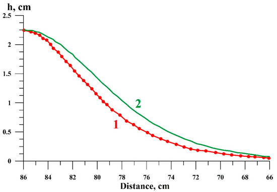
Figure 1.
Solitary wave calculation (green curve 2) and observational data (red circles). A wave with an amplitude A = 2.25 cm/s runs in a H = 6 cm depth channel. Only the right side of the wave is shown since the wave is symmetrical along the vertical axis.
Let us consider the results of the mega-tsunami in Lituya Bay (AK, USA) (Figure 2). The maximum amplitude of the wave was equal to A = 60 m, and the middle depth was H = 122 m [23,28].
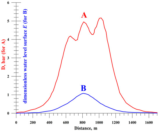
Figure 2.
Dynamic pressure D (curve A) and dimensionless water surface level E (curve B) versus distance were calculated using Formulas (28), (29), and (22) according to the model of mega-tsunami in Lituya Bay.
The dimensionless amplitude was calculated for the time t = 20 s after the onset of the tsunami. We can see in Figure 2 (curve B) that the wave has the form of a hill running at a velocity of c. Note that this velocity is greater than the speed of linear wave c0 and depends on the maximal amplitude A. Parameters D and E can be used to classify geodynamic events after tsunamis.
Analysis of the nonlinear boundary conditions [13,26] and Equation (3) shows that the potential Φ is related to depth-average velocity V by the formula
where
and the phase of the wave
Substituting (25) into (24) and considering (9), we obtain
Moreover, the pressure p(x = 0) is assumed to be absent at the origin of the coordinates.
Formulas (6) and (27) allow us to obtain the potential φ and its derivatives. Substituting the results into Formula (5), we find the pressure
The first term in relation (28) represents atmospheric pressure, which equals 101,325 Pa ≈ 1.01 bar. The second term on the right side of Equation (28) is the hydrostatic pressure, which increases linearly with depth and becomes zero at the water surface z = H. The third term on the right side of (28) depends on the phase of the wave γ and describes the pressure disturbance associated with the solitary wave. The remaining terms in (28) depend not only on the phase of the wave γ but also on the vertical coordinate z. They describe the changes in pressure with depth in a solitary wave. The maximum pressure is achieved at the bottom of the marine (oceanic) basin; the corresponding calculation formula can be easily obtained by assuming z = 0 in Formula (28).
As a specific example, Figure 2 presents the results of calculations using Formulas (22), (28), and (29) for changes in the dynamic pressure
at the bottom in, according to the model of the mega-tsunami in Lituya Bay [23,28]. The area of Lituya Bay (AK, USA) is known for sharp tsunamis [28]. For example, on 9 July 1958, an earthquake with a magnitude of M = 7.8 caused a mega-tsunami with a height of 521 m. The water rose to this height from the tsunami splashing onto the bay’s shores after a huge rock and ice fell into it. Tsunami waves with a height of about 60 m were observed in this bay in 1854, 1899, and 1936. We calculated a particular model tsunami with an amplitude of a = 60 m. The average depth of the bay was chosen to be 122 m, with a maximum depth of 220 m.
For calculations, we choose seawater density 1027.675 kg/m3, corresponding to a salinity of 35 ppm and a water temperature of 5 °C (at depths less than 200 m, the dependence of water density on pressure can be neglected). As we can see, the dynamic pressure at the bottom is a three-humped soliton (“Trident of Neptune”) with a maximum of approximately equal to 5 bar at the leading front of the wave. In this example, the static pressure at the bottom
that is, the ratio D/S = 0.385 ≈ 40%. The absolute value of pressure fluctuation from a tsunami on the ocean floor is approximately 10 bars, sufficient to initiate aftershock earthquakes in overstressed areas of the Earth’s crust.
Scientists at NASA’s Jet Propulsion Laboratory used the SWOT satellite to track the source of the rumbling seismic signals recorded in September 2023 [29]. These were not tremors but tsunami waves splashing in Greenland’s narrow fjord. While analyzing the data it collected, the scientists noticed something unusual in the narrow Dickson Fjord, part of a network of channels in eastern Greenland. It has a maximum depth of 540 m, is 2700 m wide, and has more than 1800 m high walls. SWOT found that the water levels on the northern and southern shores of the fjord differed by more than a meter, which should not happen under normal conditions.
Further work with the data showed that a giant rockfall occurred in this fjord, causing about 25 million m3 of rock and ice to collapse into the water. A powerful tsunami wave was created since the fjord is relatively narrow and enclosed. A figure similar to Figure 2 may also be calculated for this case.
The tsunami energy had nowhere to spread beyond the fjord, so the wave walked from the northern coast to the southern and back every 90 s for nine days. Moreover, its impacts were so substantial that seismic signals were recorded by stations far from Greenland. Thus, a complex mechanism for the propagation of tsunami waves caused by landslides and rockfalls was revealed here. This again demonstrates the need to develop modern physical-mathematical apparatus for assessing such dangerous natural phenomena.
Note that the above calculations relate to mega-tsunamis with large amplitudes. Such tsunamis are rare in nature. Usually, the amplitudes of tsunamis do not exceed 2 m [30]. Nevertheless, the proposed method is universal and suitable for estimating the geodynamic effects of tsunamis of any amplitude.
Thus, procedures for estimating the secondary aftershock parameters are presented here. The formulas mentioned above can assess the danger of secondary seismological events caused by the ocean’s water influence on the underlying Earth’s surface. Completing a variety of similar calculations will allow the application of a machine learning methodology [31]. We propose that the approach first described here for estimating geodynamic post-tsunami effects will obtain further elaboration.
At the same time, it should be noted that the strength and magnitude of aftershocks are, as a rule, less than the main impact of the generating tsunami. However, many known cases exist where buildings damaged by the main shock collapsed precisely during the aftershock, with less strong tremors. The aftershocks pose a significant threat during rescue operations.
Author Contributions
S.A.A. and L.V.E. made equivalent contributions to all sections of this paper. All authors have read and agreed to the published version of the manuscript.
Funding
This research received no external funding.
Data Availability Statement
The data presented in this study are available on request from the corresponding author.
Acknowledgments
The authors thank three anonymous reviewers who thoroughly reviewed the manuscript and provided valuable suggestions that helped us to prepare this paper.
Conflicts of Interest
The authors declare no conflicts of interest.
References
- Turcotte, D.; Schubert, G. Geodynamics, 3rd ed.; Cambridge University Press: Cambridge, UK, 2014; p. 636. [Google Scholar] [CrossRef]
- Khain, V.E.; Lomize, M.G. Geotectonics with Basics of Geodynamics; Moscow State University: Moscow, Russia, 1995; p. 480. (In Russian) [Google Scholar]
- Aleinikov, A.L.; Belikov, V.T.; Eppelbaum, L.V. Some Physical Foundations of Geodynamics; Kedem Printing-House: Tel Aviv, Israel, 2001; p. 172. [Google Scholar]
- Stüwe, K. Geodynamics of the Lithosphere; Springer: Berlin/Heidelberg, Germany, 2007; p. 493. [Google Scholar]
- Riguzzi, F.; Panza, G.; Varga, P.; Doglioni, K. Can Earth’s rotation and tidal despinning drive plate tectonics? Tectonophysics 2010, 484, 60–73. [Google Scholar] [CrossRef]
- Zaccagnino, D.; Vespe, F.; Doglioni, C. Tidal modulation of plate motions. Earth Sci. Rev. 2020, 205, 103179. [Google Scholar] [CrossRef]
- Popov, V.L. Mechanics of Contact Interaction and Physics of Friction. From Nanotribology to Earthquake Dynamics; Fizmatlit: Moscow, Russia, 2013; p. 352. (In Russian) [Google Scholar]
- Cox, C.J.; Cooker, M.J. The motion of a rigid body impelled by sea-wave impact. Appl. Ocean Res. 1999, 21, 113–125. [Google Scholar] [CrossRef]
- Saito, S. Tsunami Generation and Propagation; Springer: Tokyo, Japan, 2019; p. 265. [Google Scholar] [CrossRef]
- Tilling, R.I. (Ed.) Complexity in Tsunamis, Volcanoes, and Their Hazards; Springer: New York, NY, USA, 2022; p. 752. [Google Scholar] [CrossRef]
- Dodd, R.K.; Eilbeck, J.C.; Gibbon, J.D.; Morris, H.C. Solitons and Nonlinear Wave Equations; Academic Press: New York, NY, USA, 1982; p. 630. [Google Scholar]
- Newell, A.C. Solitons in Mathematics and Physics; CBMS-NSF Regional Conference Series in Applied Mathematics, Ser. No. 48; Society for Industrial and Applied Mathematics: Philadelphia, PA, USA, 1987; p. 240. [Google Scholar]
- Whitham, G.B. Linear and Nonlinear Waves; John Wiley & Sons: New York, NY, USA, 2011; p. 660. [Google Scholar] [CrossRef]
- de Jager, E.M. On the Origin of the Korteweg-de Vries Equation. arXiv 2011, arXiv:math/0602661. [Google Scholar] [CrossRef]
- Guo, B.; Pang, X.-F.; Wang, Y.F.; Liu, N. Solitons; Walter de Gruyter: Berlin, Germany; Boston, MA, USA, 2018; p. 367. [Google Scholar]
- Arsen’yev, S.A.; Eppelbaum, L.V. Nonlinear model of coastal flooding by a highly turbulent tsunami. J. Nonlinear Math. Phys. 2021, 28, 436–451. [Google Scholar] [CrossRef]
- Arsen’yev, S.A.; Eppelbaum, L.V. The Behavior of Nonlinear Tsunami Waves Running on the Shelf. New Challenges in Seismic Hazard Assessment. Appl. Sci. 2023, 13, 8112. [Google Scholar] [CrossRef]
- Arcas, D.; Segur, H. Seismically generated tsunamis. Phil. Trans. R. Soc. A. 2012, 370, 1505–1542. [Google Scholar] [CrossRef] [PubMed][Green Version]
- Assier-Rzadkiewicz, S.; Heinrich, P.; Sabatier, P.C.; Savoye, B.; Bourillet, J.F. Numerical modelling of a landslide-generated tsunami: The 1979 nice event. Pure Appl. Geophys. 2000, 157, 1707–1727. [Google Scholar] [CrossRef]
- Suppasri, A.; Maly, E.; Kitamura, M.; Syamsidik; Pescaroli, G.; Alexander, D.; Imamura, F. Cascading disasters triggered by tsunami hazards: A perspective for critical infrastructure resilience and disaster risk reduction. Int. J. Disaster Risk Reduct. 2021, 66, 102597. [Google Scholar] [CrossRef]
- Zengaffinen-Morris, T.; Urgeles, R.; Løvholt, F. On the inference of tsunami uncertainties from landslide run-out observations. J. Geophys. Res. Ocean. 2022, 127, e2021JC018033. [Google Scholar] [CrossRef]
- Lo, P.H.-Y. Analytical and numerical investigation on the energy of free and locked tsunami waves generated by a submarine landslide. Phys. Fluids 2023, 35, 046601. [Google Scholar] [CrossRef]
- Korsgaard, N.J.; Svennevig, K.; Søndergaard, A.S.; Luetzenburg, G.; Oksman, M.; Larsen, N.K. Giant mid-Holocene landslide-generated tsunamis recorded in lake sediments from Saqqaq, West Greenland. Nat. Hazards Earth Syst. Sci. 2024, 24, 757–772. [Google Scholar] [CrossRef]
- Smith, E.H. (Ed.) Mechanical Engineer’s Reference Book, 12th ed.; Buttenvorth-Heinemann: Oxford, UK, 2000; p. 1194. [Google Scholar]
- Tkhonov, A.N.; Samarsky, A.A. Equations of Mathematical Physics; Dover Publications: New York, NY, USA, 2013; p. 800. [Google Scholar]
- Arsen’yev, S.A. Towards the theory of long waves on water. Doklady Russ. Acad. Sci. 1994, 334, 635–638. [Google Scholar]
- Renouard, D.P.; Seabra Santos, F.L.; Temperville, A.M. Experimental study of the generation, damping, and reflation of a solitary wave. Dyn. Atmos. Ocean. 1985, 9, 341–358. [Google Scholar] [CrossRef]
- Fritz, H.M.; Mohammed, F.; Yoo, G. Lituya Bay Landslide Impact Generated Mega-Tsunami 50th Anniversary. Pure Appl. Geophys. 2009, 166, 153–175. [Google Scholar] [CrossRef]
- International SWOT Satellite Spots Planet-Rumbling Greenland Tsunami. 30 October 2024. Available online: https://www.nasa.gov/missions/swot/international-swot-satellite-spots-planet-rumbling-greenland-tsunami/ (accessed on 8 November 2024).
- Dimova, L.; Raykova, R. Tsunami Radiation Pattern in the Eastern Mediterranean. J. Phys. Technol. 2017, 1, 22–27. [Google Scholar]
- Diniz, P.S.R.; Suykens, J.A.K.; Theodoridis, S.R. (Eds.) Signal Processing Theory and Machine Learning; Academic Press: Cambridge, MA, USA, 2023; p. 1234. [Google Scholar]


Disclaimer/Publisher’s Note: The statements, opinions and data contained in all publications are solely those of the individual author(s) and contributor(s) and not of MDPI and/or the editor(s). MDPI and/or the editor(s) disclaim responsibility for any injury to people or property resulting from any ideas, methods, instructions or products referred to in the content. |
© 2024 by the authors. Licensee MDPI, Basel, Switzerland. This article is an open access article distributed under the terms and conditions of the Creative Commons Attribution (CC BY) license (https://creativecommons.org/licenses/by/4.0/).