1. Introduction
The oil and gas industry faces a dual challenge: drilling more efficiently while maximizing production. To address this, geosteering emerged as a critical technology, which involves precise control and adjustment of drilling operations to navigate through subsurface geological formations with accuracy and efficiency [
1,
2,
3,
4,
5]. This transformative technology has revolutionized well drilling and reservoir management [
6], resulting in reduced operational costs, optimized hydrocarbon production, and a minimized environmental footprint.
Geosteering, aiming at intersecting specific reservoir zones, can be dissected into three key components: predrilling planning, monitoring/model updating, and in-drilling decision-making [
7]. As the cornerstone of successful geosteering, geological interpretation involves continuous measurement, interpretation, and modeling of the formation of interest, drawing from various data sources like well-log measurements, seismic surveys, cuttings, and coring operations [
8]. More specifically, during the construction of the well, geoscientists and drilling engineers frequently analyze the collected well logs to determine lithology and resistivity of the formations surrounding the wellbore while drilling (well-log interpretation) and combine the interpretation with established larger-scale area seismic surveys to reconstruct the subsurface formation shapes (horizon tracking). The interpreted formation shapes need to be continually updated while drilling to offer real-time insights into subsurface conditions, which help drillers make informed geosteering decisions to optimize the drilled well trajectory and well placement.
However, nowadays, processes in these different phases of geosteering highly rely on human inputs, initial condition setups, and personal judgments, which can lead to suboptimal and biased drilling decisions. Moreover, given the indirect and incomplete information used in geological interpretation, uncertainties are unavoidable [
9]. Recent research has focused on probabilistic well-log interpretation techniques to address the uncertainty in geological interpretation. One prominent approach is to interpret the well-log data via Bayesian analysis. Traditional Kalman filters, ensemble Kalman filters, and Monte Calo techniques have been explored to generate probabilistic near-wellbore formation shapes. An alternative approach is to treat the interpretation as a large-scale statistical inference problem, which is generally of high dimensionality and is computationally intensive.
In geological interpretation, the wellbore itself (and the high resolution well logs taken in and around it) is only a minute feature in the entire subsurface volume that is of interest to well construction operations. To be of practical use, well-log interpretation must be interpreted in the context of a larger scale model, which in the field often comes from a seismic survey taken over a large area [
10], to accomplish the horizon tracking of subsurface formation shapes. Algorithms have been proposed to auto-track the horizon within the 3D seismic volume, and recently advanced data processing approaches are incorporated to improve the tracking accuracy and efficiency.
In this paper, we delve into the prediction and reconstruction of both near-wellbore and geological-area formation shapes, considering the uncertainty and various operational constraints of geological interpretation and geosteering in well construction. A fully automated workflow is proposed to combine well-log interpretation and horizon tracking to optimize geosteering activities. The implementation of recursive Bayesian filter for formation shape estimation is first explored. Additionally, the concept of horizon auto-tracking (a numerical algorithm for formation horizon identification in the 3D space) is introduced. Combing well logs and initial structural geomodels, it yields a stereoscopic data for geosteering process. Lastly, the proposed geosteering interpretation approach is rigorously tested, using both synthetic and field datasets, to validate its effectiveness and reliability in geosteering applications.
2. Bayesian Well-Log Interpretation
In the well-log interpretation process, the near-wellbore formation shapes are estimated by pattern-matching between the measured and modeled logging tool responses [
8,
11]. More specifically, the response of the logging tool is firstly modeled as a function of its relative location compared to the formation boundary, which is derived from an offset well log or a composite of well logs (a reference or type log). By matching the well log obtained while drilling and the established logging tool response, the near-wellbore formation shape can be reconstructed [
10].
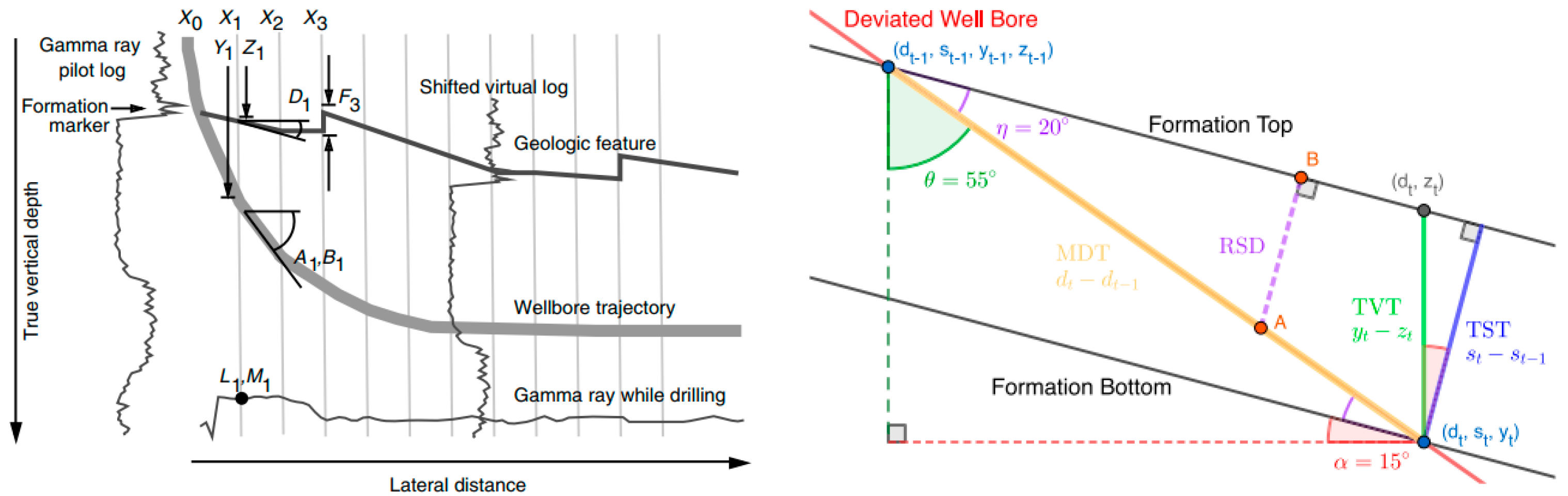
There are multiple models to describe the well-log interpretation problem and
Figure 1 below provides two examples. One example (
Figure 1, left) involves tracking the tool location, either in Cartesian coordinates or in terms of its True Vertical Depth (TVD), inclination, and azimuth [
12]. Additionally, it involves monitoring the formation’s dip angle and the fault throw (i.e., sudden vertical displacement) at each location along the wellbore. Another example (
Figure 1, right) also employs the logging tool’s location, but instead of considering the dip angle or fault throw, it utilizes the concept of Relative Stratigraphic Depth (RSD) to represent the location of the formation boundary [
13].
In the field operation, recursive Bayesian filtering is becoming a common approach used to generate probabilistic geological interpretations for geosteering. One of the earliest examples in the literature is [
7], which uses the traditional Kalman filter to estimate the distance to formation boundaries along the lateral section of a wellbore, utilizing resistivity measurements. Resistivity is a common well-log measurement that is produced by the resistivity tool, which uses current flow in a coil to induce current flow in the formation under investigation to measure the formation. Various information, such as formation porosity, water saturation, presence of hydrocarbons, etc., can be inferred from the resistivity well logs. In [
14,
15,
16], the response of a resistivity tool to the formation rock is modeled as an electro-magnetic simulator and the ensemble Kalman filter (EnKF) is adopted to estimate the formation boundaries. More recent publications [
13,
17,
18,
19] adopted sequential Monte Carlo techniques (i.e., particle filters) as a substitution of the Kalman filter. However, these aforementioned interpretation techniques only estimate the distance to or shape of nearby formation boundaries in the near-wellbore field. There is no consideration of the formation boundaries far away from the wellbore, which limits the application of the recursive Bayesian filtering for further steering decision optimization.
Other recent well-log interpretation approaches use similar formation boundary models in
Figure 1, but unlike recursive Bayesian filters which solve the estimation problem sequentially, they solve a larger-scale inference problem, see [
12,
20,
21]. Given a prior estimate of the formation boundaries (or some representation of the boundaries) along with new measurements taken along the wellbore, these methods infer the posterior distribution of the formation boundaries over the entire wellbore. However, due to the high dimensionality of this problem, the proposed model representations and solution methods are computationally intensive and do not always offer significant improvements over the most efficient recursive Bayesian filtering methods [
13].
4. Methods
As discussed in the previous section, while neither well logs nor initial structural geomodels are sufficient on their own to drive real-time geosteering optimization, together they form the basis of real-time geosteering interpretation and decision making. The initial structural model can be used to generate an initial planned trajectory. During the drilling process, the well log is interpreted against one or more offset wells and is adopted to update the formation boundary estimations. In this session, an automated 3D formation boundary interpretation approach, combining well logs and seismic image data, is described in detail.
Similar to the work in [
13,
19], in this work a particle filter is used to address the well-log interpretation problem. The states of interest are inclination
, azimuth
, TVD
, true stratigraphic thickness (TST) of the formation
, and RSD between the logging tool and the upper formation layer
of the logging tool at the station
. The RSD is the distance between the wellbore and the formation boundary measured in the direction of the formation layer’s TST as shown earlier in
Figure 1.
The discrete system dynamics of the tool location are computed using the wellbore survey and minimum curvature method (MCM) to estimate the changes in the tool’s location and orientation. MCM is used to interpolate inclination and azimuth, and TVD between survey stations:
where
is the additive Gaussian noise affecting the system dynamics and the subscript indicates that each state’s dynamics function (
,
,
, and
) is associated with a different noise term;
is the change in measured depth between points
and
along the wellbore. The dynamics of the formation boundaries are represented using the Setchell equation [
10], which relates the change in measured depth thickness (MDT) along the wellbore to changes in TST of the formation as follows:
where
is the dip for the formation and
is the strike of the formation. This relationship is illustrated in
Figure 1 (right). However, in the example shown in the figure, it is assumed that
aligns with
, so these terms are not shown. Given a sufficiently small increment of measured depth, the change in RSD can be approximated by the change in TST as:
The system observation equations are given by:
where
is the additive Gaussian noise affecting the system observations
at time
;
is a mapping between RSD and the associated type log responses;
and
are scale and shift factors, which are often necessary to account for differences between the type log and the MWD log caused by their calibration (or lack thereof);
is the predicted log response. Realizations of the filter state vector and measurement vector are:
where
is the state vector of the nth particle in the filter at time
;
is the overall measurement vector at time
.
In [
13], the authors proposed the use of expectation maximization or Gibbs sampling to approximate
and
as static hidden states, which, however, is computationally intensive. Here, an alternative procedure is proposed to estimate these factors. First, the wellbore and type logs are aligned using dynamic time warping. Then, a linear transformation (i.e.,
) is fit using the method of least squares to match the magnitude of the type log responses to the MWD log responses. This provides estimates of the
and
parameters that correct for potential shifting and scaling between the log responses. After estimating the RSD and thickness parameters, the TVD of the upper and lower target formation boundaries,
and
, respectively, can be found at each point along the wellbore using the following equation:
The particle filtering process makes use of these system equations (Equations (1)–(4), (6)–(9)) and sensor measurements to estimate a discrete, multi-dimensional distribution over the state vector at each point along the wellbore. The particle filter is a parameter free, recursive Bayesian filter [
31] and achieves the estimation by maintaining a particle set or a list of state vectors. At each iteration, the filter samples a new set of particles from the prior state vector distribution by applying the dynamics equations to the current set of particles. Each particle is then used to predict the next sensor measurement. The particles are then weighted based on the prediction difference and the weights are normalized to sum of one. This is followed by a process known as resampling in which the particle set is replaced by a random sampling from the current distribution and the sampling probability of each particle is equal to its normalized weight value. This new set is the posterior distribution of particles at the current time step (i.e., the current state vector probability distribution).
In the proposed approach, Augmented Monte Carlo Localization (AMCL) and Kullback–Leibler divergence (KLD) sampling [
31] are also utilized for improvements against classical particle filters. AMCL helps to prevent degeneracy of the particle set, which is commonly due to repeated resampling. It randomly replaces old particles in the set with random samples from the support of the state space (i.e., the set of feasible values of particle states). Meanwhile, KLD sampling adaptively increases/decreases the size of the particle set to reduce the error in the particle set’s estimation of the target distribution. This helps to keep the filter both accurate and efficient as it always uses a sufficient number of particles.
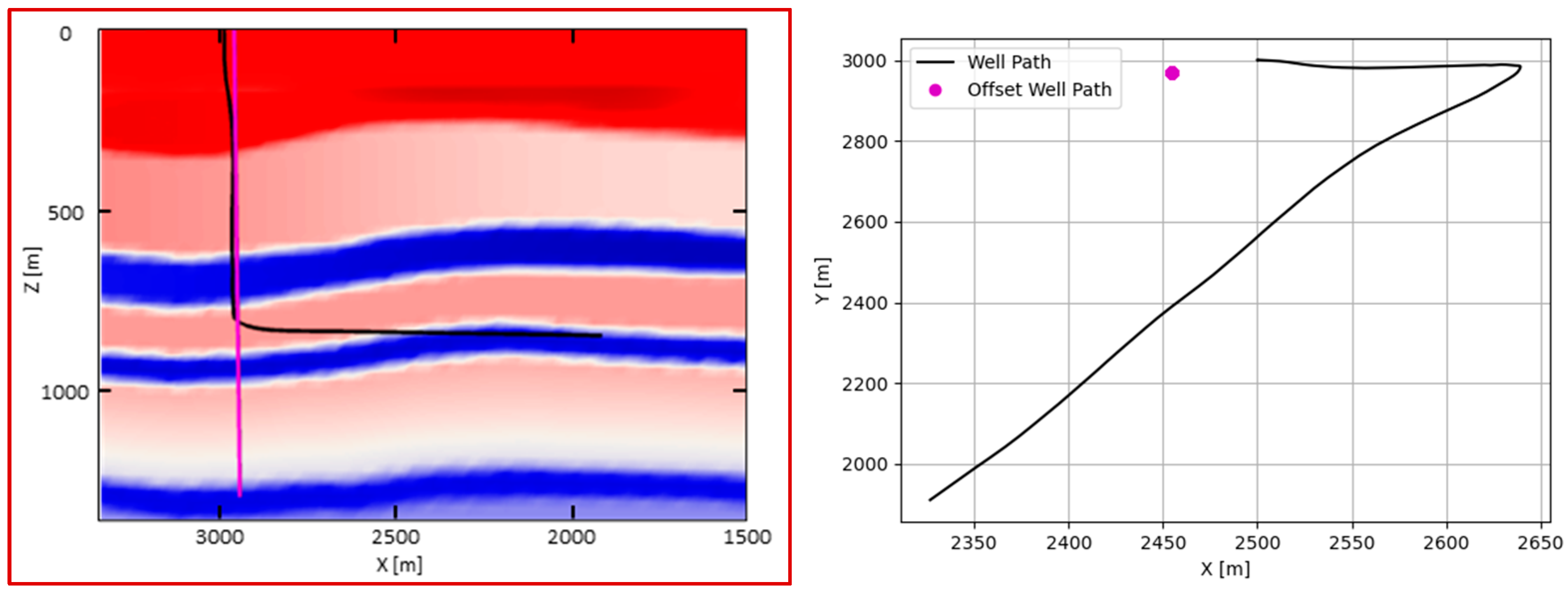
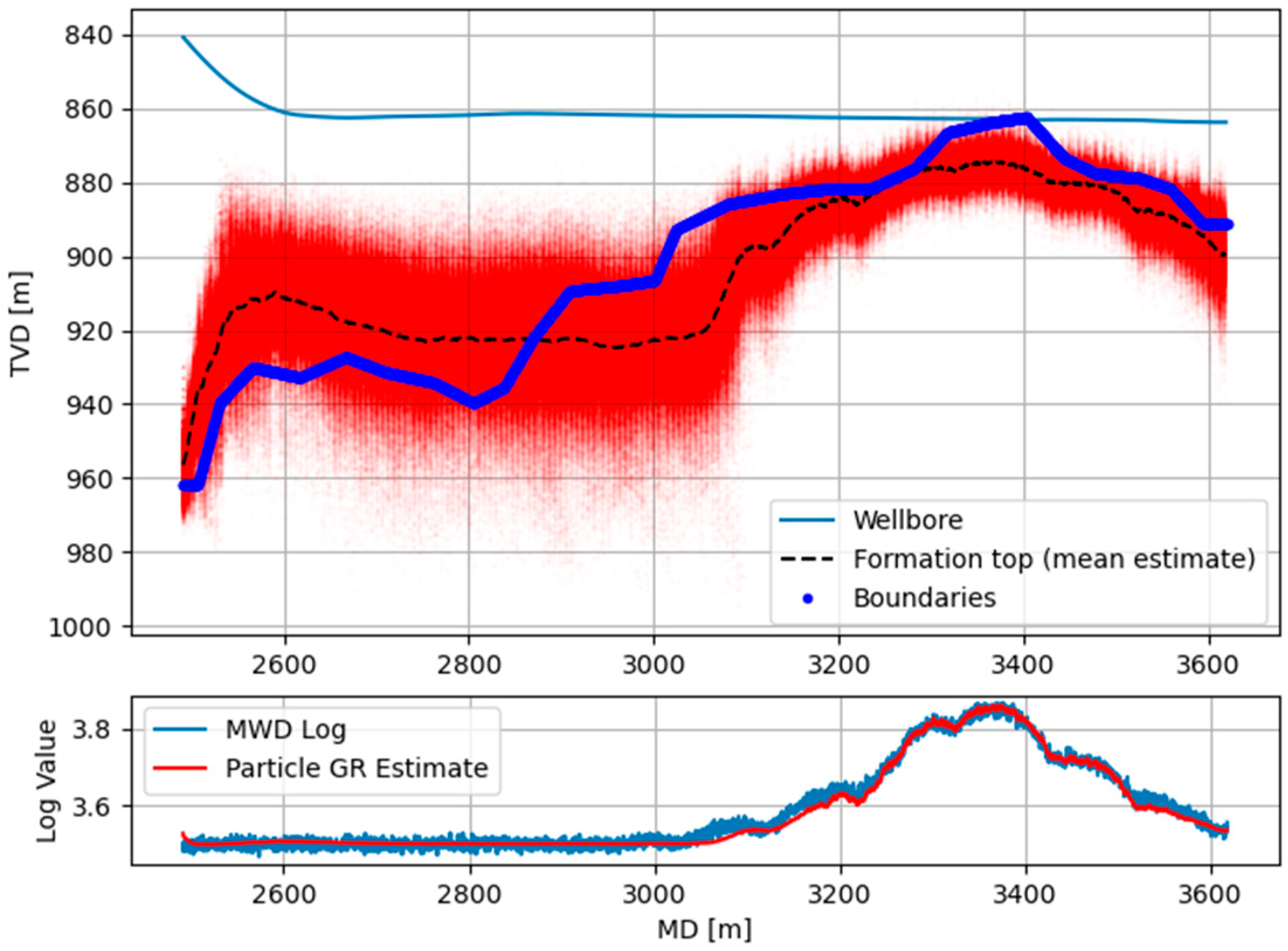
The particle filtering method described above provides an estimate of the RSD separating the wellbore and one or more formation boundaries. Since this analysis is only performed using the one-dimensional log measurement taken along the wellbore, the boundaries lie along a two-dimensional surface following the wellbore as shown in
Figure 5.
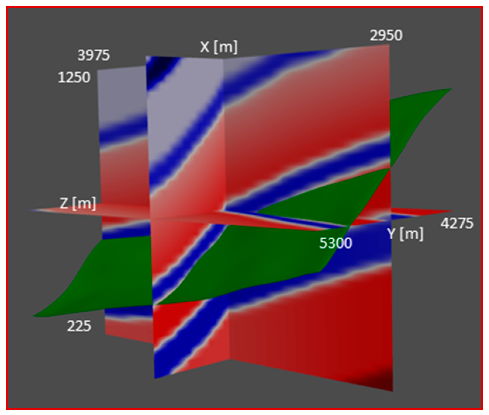
In the 3D formation boundary estimation, boundary points estimated above by the particle filter are used as control points for the horizon tracking algorithm [
32]. A 3D surface is approximated conforming to the structure present in the seismic image as illustrated in
Figure 6. In this process, the assumption of 2D boundary continuity produced from the particle filter is removed and a surface that conforms to the near-wellbore interpretations made by the particle filter and that follows the seismic formation structure further from the wellbore is tracked. More specifically, careful consideration is required when interpreting through faults or unconformities [
33] and in this work a horizon across the entire seismic volume is tracked using a constrained, least-squares method.
Similar to how a grayscale picture image is a set of intensity values on a uniform 2D grid, a seismic image is a set of intensity values defined along a uniform 3D grid. The changes in these intensity values represent the structural layout of the subsurface formations and a surface or horizon is represented as a collection of depth with an entry , for every location along the seismic grid. It is also convenient to refer to the set of control points as another collection of depth values , containing the depth value associated with each control point’s grid location.
As shown in
Figure 7, the seismic reflector slopes, denoted as
and
, also referred to as inline and crossline dip values, are computed at each point within the seismic image volume using the structure tensor
:
where
represent the components of the image gradient vector computed within the neighborhood of a point in the 3D image; 〈∙〉 signifies a weighted sum of the contents within the brackets. In practice, this convolution operation is often performed using Gaussian smoothing techniques and the eigen decomposition of the structure tensor
provides an estimate of the orientation vectors of the seismic reflector surfaces:
where
and
are the normalized eigenvectors of
;
and
are the eigenvalues of
. Assuming
, then
is the normal vector to the seismic reflector surface while
and
are tangent vectors pointing along the surface. The computation of seismic reflector slopes can be derived from the components of the
as:
where
are the vertical, inline, and crossline components of the vectors in
, respectively, and the dip azimuth
can be calculated as:
The eigenvalues
and
can also be used to derive the local horizon planarity
, which is a value between zero and one and is high near planar regions of the formation and low near discontinuities or faults [
34,
35]:
In the horizon tracking algorithm, a horizon is assumed to follow the structure of the seismic image when the derivatives
and
at the associated 2D coordinate
follow the corresponding seismic reflector slopes:
where
and
denote the seismic reflector slopes
and
computed at the 3D coordinate
. In practical scenarios, this assumption is likely to be violated, especially near faults or discontinuities in the seismic image. To address this issue, the relationship described above is weighted by a measure of local planarity, denoted as
. Additionally, due to the presence of noise in the seismic image, it may be necessary to regularize the least-squares problem using a small constant,
:
Based on Equations (12)–(20), the least-squares method seeks to determine the horizon
, that adheres to the slopes within the seismic image, which can be expressed in matrix form as follows:
where
and
are the matrix representations of the finite-difference approximations of the 2D gradient and Laplace (i.e., second-order gradient) operators, respectively;
is a diagonal matrix containing the weights
;
is a vector concatenated by reflection slopes
and
for
;
is the constraint enforcing that the surface must pass through the
control points defined by the well logs; subscripts
and
indicate the dependence of the problem on the current or ith estimate of the horizon (
). Every time solving the problem yields a new estimate of the surface
and this iteration process is necessary because the weighting term
and reflection slopes
depend on the unknown vector
.
This least-squares problem is solved iteratively from an initial guess using the preconditioned conjugate gradient method until the change in the surface estimate between iterations converges below a fixed tolerance. Preconditioned conjugate gradient is ideal for this problem because it allows the constraints to be enforced through the preconditioner matrix and because the system of equations being solved is large and very sparse [
32]. The initial guess is found using a nearest-neighbor extrapolation of the depth values of the control points at each
location along the seismic image grid (i.e., the nearest control point’s
value becomes the initial guess for the
value at each point along the
seismic image grid).
In conclusion, with the proposed well-log interpretation and horizon tracking algorithm, the geosteering interpretation workflow is illustrated in
Figure 8. The workflow can be repeated whenever new log and survey measurements become available.


 ,
, 


