Article

Possible Interrelations of Space Weather and Seismic Activity: An Implication for Earthquake Forecast

by
Valery Sorokin
1 and
Victor Novikov
2,3,*
1
Pushkov Institute of Terrestrial Magnetism, Ionosphere, and Radio Wave Propagation, Russian Academy of Sciences, Moscow 108840, Russia
2
Joint Institute for High Temperatures, Russian Academy of Sciences, Moscow 125412, Russia
3
Sadovsky Institute of Geospheres Dynamics, Russian Academy of Sciences, Moscow 119334, Russia
*
Author to whom correspondence should be addressed.
Geosciences 2024, 14(5), 116; https://doi.org/10.3390/geosciences14050116
Submission received: 23 February 2024 / Revised: 21 April 2024 / Accepted: 24 April 2024 / Published: 25 April 2024

Abstract

:
The statistical analysis of the impact of the top 50 X-class solar flares (1997–2024) on global seismic activity as well as on the earthquake preparation zones located in the illuminated part of the globe and in an area of 5000 km around the subsolar point was carried out. It is shown by a method of epoch superposition that for all cases, an increase in seismicity is observed, especially in the region around the subsolar point (up to 33%) during the 10 days after the solar flare in comparison with the preceding 10 days. The case study of the aftershock sequence of a strong Mw = 9.1 earthquake (Sumatra–Andaman Islands, 26 December 2004) after the solar flare of X10.16 class (20 January 2005) demonstrated that the number of aftershocks with a magnitude of Mw ≥ 2.5 increases more than 17 times after the solar flare with a delay of 7–8 days. For the case of the Darfield earthquake (Mw = 7.1, 3 September 2010, New Zealand), it was shown that X-class solar flares and M probably triggered two strong aftershocks (Mw = 6.1 and Mw = 5.9) with the same delay of 6 days on the Port Hills fault, which is the most sensitive to external electromagnetic impact from the point of view of the fault electrical conductivity and orientation. Based on the obtained results, the possible application of natural electromagnetic triggering of earthquakes is discussed for the earthquake forecast using confidently recorded strong external electromagnetic triggering impacts on the specific earthquake preparation zones, as well as ionospheric perturbations due to aerosol emission from the earthquake sources recorded by satellites.

1. Introduction

The problem of a possible relation between solar activity and the Earth’s seismicity has been discussed over 170 years [1,2,3,4,5,6,7,8,9], with references therein. Despite a fairly large number of publications devoted to research on the possible influence of the Sun on seismic processes, a final conclusion about the possibility of earthquakes (EQs) being triggered by solar flares (SFs) or geomagnetic storms has not yet been reached. The results obtained to date are fuzzy and contradictive, and some authors deny the real existence of interrelationships between the processes in the Sun and in the lithosphere that resulted in the occurrence of EQs [10,11].
It should be noted that all the studies mentioned above employed only a statistical approach to the analysis of geophysical and seismological data when the hypothesis of the presence or absence of a possible correlation (positive or negative) between solar activity and Earth’s seismicity was tested. The physical mechanisms of solar–terrestrial relations that resulted in the possible triggering of EQs were not considered in detail, and their possible existence was only indicated phenomenologically when a statistically significant relationship has been found between solar activity and the response of the Earth’s seismicity. Such a simplified approach to the study of the solar–terrestrial relationships may provide false results and incorrect conclusions, and no practical recommendations may be proposed for seismic risk mitigation.
In contrast to a pure statistical approach, the study of Sorokin et al. [12] considers a possible physical mechanism of earthquake (EQ) triggering by electromagnetic (EM) impacts on the area of EQ preparation due to X-ray radiation from SFs. This idea has been proposed in Sorokin et al. [5] and Novikov et al. [7], when it was numerically demonstrated that due to the interaction of SF X-ray radiation with the ionosphere–atmosphere–lithosphere system, strong geomagnetic field pulsations occur, resulting in the sharp rise of geomagnetically induced currents (GICs) in the conductive crust faults. It is known that EQs can be triggered by strong variations in both natural and artificial electric currents in the Earth’s crust as a result of the interaction of EM and electric fields with rocks and faults under subcritical stress–strain state [13].
The results of numerical studies obtained in Sorokin et al. [12] using the developed physical model and computer code indicate that after an X-class SF (with peak radiation flux ≥10−4 W/m2), geomagnetic field pulsations up to 100 nT can occur, and the density of GICs in the conductive layer of the lithosphere can rise to 10−8–10−6 A/m2. In this case, the current pulse duration is about 100 s and the duration of the current rise front is ~10 s. These values are 2–3 orders of magnitude higher than the average density of telluric currents in the lithosphere [14] and they are comparable with the parameters of electric current pulses generated in the lithosphere (10−7–10−8 A/m2) by artificially pulsed sources of electrical energy [13]. It should be noted that the injections of electrical impulses into the Earth’s crust in seismically active regions result in the EM triggering of weak EQs and the regional spatiotemporal redistribution of seismicity in the Pamirs and Northern Tien Shan. This means that strong SFs providing an energy flux density above 0.005 J/m2 are also capable of triggering EQs in seismically hazardous regions, as was assumed in [7,12,15]. This conclusion is confirmed by cases of observation of magnetic pulses before an EQ [16,17] similarly to the obtained numerical estimates of magnetic pulses generated by X-rays of SF provided telluric current pulses in the conductive layer of the lithosphere, as well as the case of observation of a sharp increase in global and regional seismicity (Greece) after the SF of X13.37 class that occurred on 6 September 2017 [7].
For additional verification of numerical results obtained with the application of the physical model of the Sun–Earth interaction [12], we carried out the statistical analysis of the impact of the top 50 X-class SFs on global seismic activity, the EQs located on the illuminated part of the globe and the EQs located in an area of 5000 km around the subsolar point (SSP). We demonstrated that in all cases, an increase in seismicity is observed, especially in the region around the SSP (up to 33%) during the 6–8 days after the SF. Moreover, we found that the maximum seismic sensitivity to the SF impact is observed in the aftershock area of the strong EQ. The case study of the aftershock sequence behavior of strong Mw = 9.1 EQ (Sumatra–Andaman Islands, 26 December 2004) after the X10.16-class SF (20 January 2005, peak radiation flux is 10.16 × 10⁻⁴ W/m2) demonstrated that starting from the 7th day after the SF, the number of aftershocks with a magnitude of Mw ≥ 2.5 increased more than 20 times by the 8th day and returned to the background level within the following two days. In addition, we consider the case of the Darfield EQ (4 September 2010, Mw = 7.1, New Zealand) with two strong aftershocks (Mw ~ 6) occurring in the Port Hills fault, which were most sensitive to external EM impact from the point of view of the fault electrical conductivity and orientation, with a delay of 6 days after strong X-class SFs and M.
Finally, based on the obtained results, we discuss the possibility of applying natural EM triggering of EQs for the EQ forecast, using confidently recorded strong external EM triggering impacts on the specific electromagnetically sensitive EQ preparation zones.

2. Methods of Verification of Hypothesis of Electromagnetic Earthquake Triggering by Strong X-Class SFs

2.1. Testable Hypothesis of Earthquake Triggering by Strong SFs

In Sorokin et al. [5], Novikov et al. [7], and Sorokin et al. [12], a possible mechanism of EQ triggering by the ionizing radiation of SFs has been proposed. The theoretical model of Sorokin et al. [12] considered a disturbance of electric field, electric current, and heat release in the lithosphere associated with a variation in ionosphere conductivity caused by the absorption of ionizing radiation from SFs. The model predicted the generation of geomagnetic field disturbances in a range of seconds to tens of seconds as a result of a large-scale perturbation of the conductivity of the bottom part of the ionosphere in a horizontal direction in the presence of an external electric field. Amplitude-time characteristics of the geomagnetic disturbance depend upon a perturbation of the integral conductivity of the ionosphere [12]. Numerical calculations demonstrated that, depending on the relationship between the integral Hall and Pedersen conductivities of the disturbed ionosphere, oscillating and aperiodic modes of magnetic disturbances may be observed. For strong perturbations of ionosphere conductivities, the amplitude of pulsations may be ~102 nT. In this case, the amplitude of the horizontal component of the electric field on the Earth’s surface will be 0.01 mV/m, and the electric current density in the lithosphere may reach 10−6 A/m2 [12]. Thus, it was shown that the absorption of ionizing radiation from SFs can result in variations of a density of telluric currents in seismogenic faults comparable with a current density of 10−8–10−7 A/m2 generated in the Earth’s crust by artificial pulsed power systems (geophysical MHD generator “Pamir-2” and electric pulsed facility “ERGU-600”), which provided regional EQ triggering and spatiotemporal variation of seismic activity [13]. Therefore, we can expect that the triggering of seismic events is possible not only due to the EM impact of the artificial pulsed power sources on the lithosphere but also due to SFs. Based on the theoretical study above mentioned and the numerical results obtained with the employment of the theoretical model [12], the hypothesis was put forward about the triggering of EQs by strong SFs under certain favorable conditions (the electrical conductivity of the fault in the Earth’s crust, its orientation relative to the direction of the GIC density vector, and the level of stress–strain state of the fault, e.g., its maturity for the dynamic rupture). This study is directed at the verification of the hypothesis by the analysis of variations in the geomagnetic field recorded at INTERMAGNET observatories during strong X-class SFs, as well as by analysis of seismicity behavior after the flares.

2.2. Analysis of Geomagnetic Field Variations and Seismic Activity during Strong X-Class SFs

According to the theoretical model [12], SF X-ray radiation will be absorbed in the ionosphere, resulting in a short-term increase in its conductivity (Figure 1, reproduced from [12]) and disturbances of the geomagnetic field in various ranges of periods in the presence of an external electric field. It was assumed that the maximal currents in the lithosphere are induced by short-period oscillations of the geomagnetic field. The “earth-ionosphere” resonator generates the geomagnetic field oscillations with periods of 1 to 100 s in the process of ionosphere ionization by SF radiation with a short-term increase in its amplitude.
Considering that the increase in ionosphere conductivity occurs on the illuminated part of the globe, we analyzed the records of the INTERMAGNET observatories [18] that were located there during SFs from the catalog of the 50 strongest X-class SFs with a peak X-ray intensity of above 10−4 W/m2 [18]. The coordinates of the SSP and the area of the illuminated part of the globe were determined by a solar calculator [19].
For the verification of the proposed model and the obtained numerical results [12] on the possible triggering of EQs by SFs, an analysis of the Earth’s seismicity before and after the strongest X-class SFs was carried out. A representative part of the US Geological Survey (USGS) EQ catalogue (Mw ≥ 4.5) [20] and a catalogue of the 50 strongest X-class SFs [21] for the period 1997–2024 were used.
The analysis of the possible correlation between SFs and EQs employed the epoch superposition method, when for the time windows of 10 days before and after the arrival of X-rays from the SF to the Earth (~8 min), all EQs that occurred in the selected region of the Earth’s crust were summed up for each day. In accordance with the physical model [12], according to which the maximum burst of telluric currents in the Earth’s crust should occur on the illuminated part of the globe, the seismicity of two regions with a center in the SSP and radii of 5000 km and 10,000 km was analyzed. The SSP coordinates were determined by the date and time of the SF occurrence.

3. Results of Verification of Hypothesis of Earthquake Triggering by Strong Solar Flares

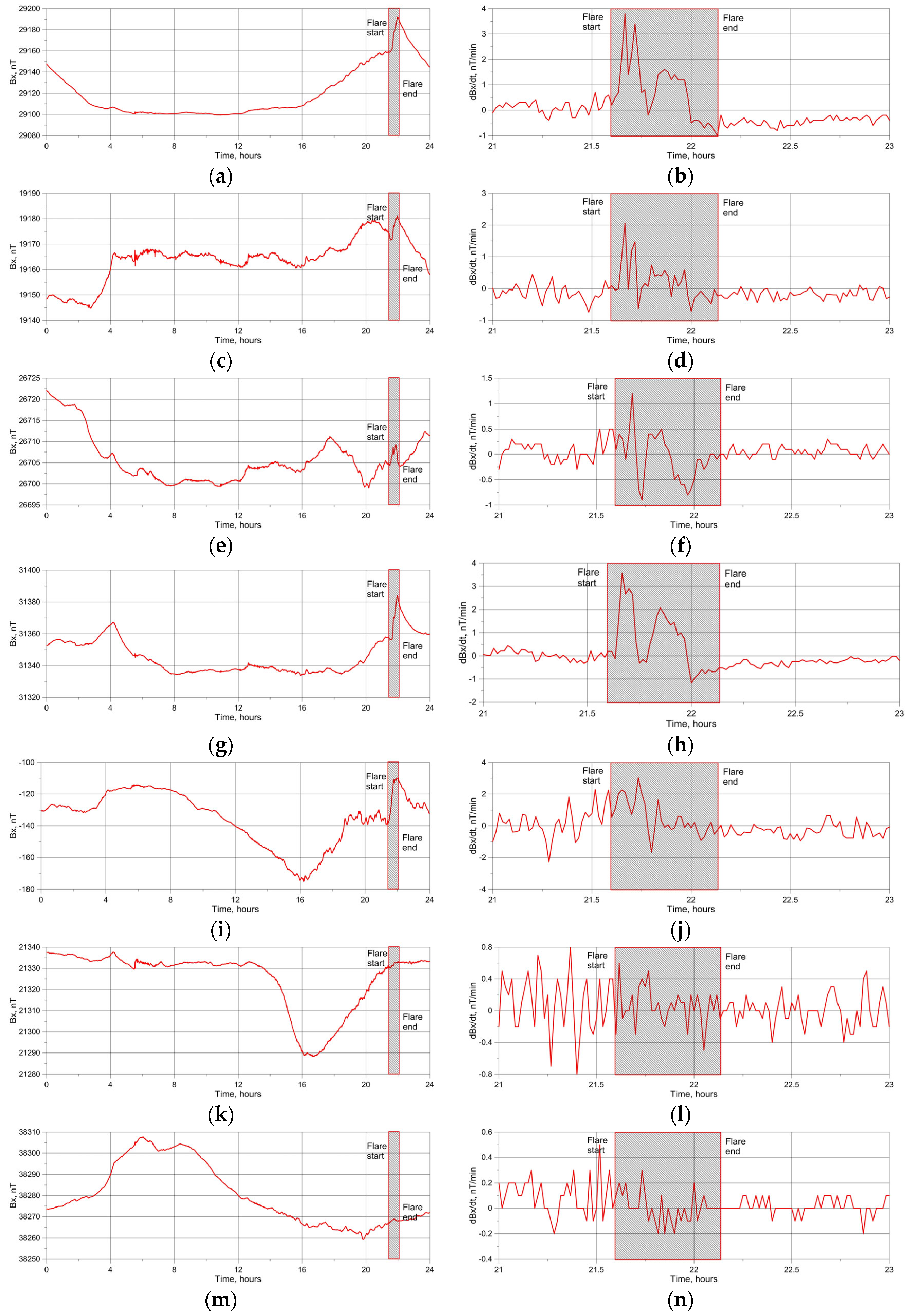
3.1. Response of Geomagnetic Field to Strong Solar Flare: The Case Study of Solar Flare X5.01 of 31 December 2023

We considered the behavior of the geomagnetic field (Bx) during strong SF X5.01 on 31 December 2023. The SF occurred at 21:36 UTC, the maximal X-ray flux was reached at 21:55 UTC, and the end of the SF was at 22:08 UTC (Figure 2).
According to the model [12], we analyzed the recordings of geomagnetic observatories located just near the SSP (23.067° S, 147.733° W) at a distance of 640.96 km and at distances of 4287.45 to 10,003.97 km (on the illuminated part of the globe at the moment of the SF) and on the non-illuminated part of the globe at a distance of 15,780.24 km from the SSP (Table 1). We considered records of the horizontal component Bx of the geomagnetic field and its derivative dBx/dt, keeping in mind their maximal contribution to GICs in the lithosphere [22]. The magnetograms for different geomagnetic observatories at different distances R from the SSP Bx (a), (c), I, (g), (i), (k), (m), and dBx/dt (b), (d), (f), (h), (j), (l), (n) for the time around the SF occurrence downloaded from the INTERMAGNET site [18] for 31 December 2023 are shown in Figure 3. The SF duration is depicted by a shadowed rectangle.
The analysis of the recorded variations in the geomagnetic field in different parts of the globe (illuminated and non-illuminated) at various distances from the SSP demonstrated that the Bx and dBx/dt pulses predicted by the model [12] during the SF were observed on the illuminated part of the globe.
At the same time, there were no geomagnetic field pulses during the X-class SF on the border of the illuminated part (FRD observatory) and on the non-illuminated part. A sharp increase in Bx during the SF totaled 20–25 nT, and dBx/dt pulsations totaled 1–4 nT/min. These observations confirmed the numerical results obtained with the employment of the model [12], that the pulses of the geomagnetic field were generated by the X-ray radiation of the SF and resulted in GIC occurrence in the lithosphere were not anticipated in the non-illuminated part of the globe. Thus, the analysis of the response of seismic activity to SFs should consider only the illuminated part of the globe. The next question arises: “Are the observed pulsed variations in the geomagnetic field capable of provoking EQs according to the hypothesis of the EM triggering of EQs by strong SFs?”

3.2. Seismic Activity before and after Strong X-Class SFs

For the analysis of the possible response of seismic activity to the impact of strong SFs, we used the representative part (Mw ≥ 4.5) of the USGS earthquake catalog [21] and a catalogue of the 50 strongest X-class SFs [19]. The analysis of the possible correlation between SFs and EQs employed the epoch superposition method, when for the time windows of 10 days before and after the arrival of X-rays from the SF to the Earth, all EQs occurring in the selected region of the Earth’s crust were summed up for each day. In accordance with the physical model [12], when the maximum burst of telluric currents in the Earth’s crust was anticipated in the illuminated part of the globe, we considered seismic activity in two circular regions with a center in the SSP and radii of 5000 km and 10,000 km (the illuminated part of the globe) and compared the results with the Earth’s overall seismicity. The detailed list of specific SFs and the analyzed possible seismic responses is given in Appendix A (see Table A1).
The summary results based on the detailed Table A1 are shown in Table 2, where ΣR=5000 is the sum of the EQs in an area with a radius of 5000 km around the SSP, ΣR=10,000 is the sum of the EQs in an area with a radius of 10,000 km around the SSP, Σglobal is the sum of EQs for the whole globe, a is the cumulative number of EQs occurring within 10 days after the SF, b is the cumulative number of EQs occuring within 10 days before the SF, and ΔEQ is the increase in the number of EQs after the SF (%).
The analysis of the values in Table 2 demonstrated that, according to the physical model and the results of the numerical studies obtained with its application [12], there was a significant seismic response in the illuminated part of the Earth. The maximum increase in the number of EQs (32.92%) was observed in the region with a radius of 5000 km around the SSP. As the radius of the region increased to 10,000 km, which is equivalent to the entire illuminated area of the globe, seismic growth decreased to 10.99%, similar to a decrease in geomagnetic field variations (see Section 3.1). In comparison with the global seismicity, the ΔEQ for the illuminated part was one and a half times higher. The histogram of the distribution of the daily number of EQs before and after the SF is shown in Figure 4. It should be noted that the increase in seismicity for the illuminated area of the globe was observed with a delay of 7–8 days after SF occurrence (Figure 4a,b) similar to a few-day delay in the response of seismic activity to the impact of artificial EM on the Earth’s crust [13].
One of the general conditions for the triggering effect of EM on the earthquake preparation zone is the level of stress–strain state of rocks and the crust fault, which, according to the results of laboratory modeling [13], should be 0.98–0.99 of the critical stresses when the dynamic rupture of the fault occurs. The current level of stresses in a particular region of the globe can be roughly estimated by indirect signs, e.g., by the current seismic activity that is used by methods of mid-term earthquake forecasting [23].
However, there are situations when it is possible, with a high degree of probability, to determine areas where subcritical stresses arise regularly in the Earth’s crust. Such areas are the aftershock zones of strong EQs. Aftershocks are a sequence of seismic events that occur after a larger main earthquake around the fault zone of the main shock. Aftershocks are a consequence of the stress field redistribution in the Earth’s crust after the main displacement along the fault as the result of the main shock. In the aftershock zone, areas occur constantly where the stresses in the Earth’s crust will be close to critical values when the rock rupture (aftershock) occurs. Aftershocks become less frequent over time, although they may continue for days, weeks, months, or even years [24]. Thus, due to the indicated stress redistribution in the aftershock zone, areas with a subcritical stress–strain state always appear, which are most sensitive to triggering impacts. In this case, when such an area is located near the SSP during the occurrence of a strong SF, it is possible to anticipate the EM triggering of aftershocks. In this regard, to verify the hypothesis of the EM triggering of earthquakes by SFs, it is quite reasonable to consider the seismic activity in the aftershock zones located near the SSP at the time of the SF occurrence.
As a case study, we considered the impact of the X10.16 SF of 20 January 2005 on the aftershock zone of the Sumatra–Andaman Mw = 9.1 EQ that occurred on 26 December 2004. The aftershock zone [25] is covered by the area of the 5000 km radius around the SSP of the X10.16-class SF (20.083° S, 77.767° E) (Figure 5). The distance from the SSP to the epicenter of the Mw = 9.1 EQ is 3306.36 km.
The histogram of the daily distribution of the aftershocks after the main shock of 26 December 2004 is shown in Figure 6. The redistribution of stresses in the crust just after the Mw = 9.1 EQ triggered many aftershocks during the first two days (269 and 202), then the daily aftershock number was reduced up to an average number of about 14, and after the X10.16 SF, with a delay of 6 days, we observed a sharp increase in seismic activity that lasted four days, with two peaks of 244 and 240 aftershocks during 27–28 January 2005. Thus, for favorable conditions from the point of view of the generation of geomagnetic field pulsations (for this case recorded at the PHU observatory located at a distance of 2933.4 km from the SSP and 2248.2 km from the Mw = 9.1 EQ epicenter, Figure 7), as well as for the zone with subcritical stress values close to the fault rupture (aftershock zone), we observed a clear EQ triggering effect of the X10.16-class SF.
It should be noted that during the month before the sharp intensification of the aftershock sequence in the period of 27–29 January 2005, there were no strong EQs in the immediate vicinity of the region under study (and throughout the entire globe) with a magnitude of Mw ≥ 7, which could provide a distant dynamic triggering effect in the considered aftershock area.
There were a few space weather disturbances due to seven SFs that occurred after the Sumatra–Andaman Mw = 9.1 EQ (see Table 3). Nevertheless, the EM impact on the aftershock zone of the strong EQ can only be attributed to the X10.16 SF of 20 January 2005 (Figure 7), due to its X-ray radiation that exceeded the other SFs 5 to 10 times and the distance from its SSP to the epicenter of the main shock that was two times less than the similar distance of the strong X5.51 SF of 17 January 2005. Nevertheless, for this case, the combined action of both SFs (X10.16 and X5.51) may be considered, which can explain the beginning of the increase in aftershocks on 26 January 2005 (see Figure 6).
Thus, this case study of aftershock sequence variation due to the impact of a strong SF indicates that, if the aftershock zone is located near the SSP during the occurrence of a strong SF (Figure 5), we can expect the EM triggering of aftershocks, which can have a magnitude comparable to that of the main shock, and they are also dangerous, especially during rescue operations after a catastrophic EQ. For the Sumatra–Andaman Mw = 9.1 EQ, the maximal magnitude of the aftershocks was Mw = 6.3.
The obtained results are supported by the occurrence of strong aftershocks after X- and M-class SFs in the New Zealand region in 2011. A strong Mw = 7.1 EQ occurred on 3 September 2010 near Darfield on the South Island of New Zealand [26], which injured about 100 people. After this EQ, an aftershock sequence began, which included a strong Mw = 6.1 aftershock that occurred on 21 February 2011 and killed 185 people. It should be noted that 6 days before this strong aftershock, an X2.3-class SF occurred (15 February 2011, 01:44–02:06 UTC) when New Zealand was in the central zone of the illuminated part of the globe at a distance of 3853.7 km from the SSP to the Mw = 6.1 aftershock epicenter. The EYR observatory (New Zealand) recorded geomagnetic field pulsations during the SF of about 20–25 nT.
According to the results of calculations using the model [12], the GIC density vector in this region had a southeastern direction and was at a level of 10−7 A/m2, which was comparable to the GIC density created in the Earth’s crust by an MHD generator and resulted in the triggering of EQs in the northern Tien Shan [13]. In the case of New Zealand, the GIC density vector coincided with the direction of the strike of the Port Hills fault [27], where a strong aftershock occurred. Thus, for an EQ to be triggered by a SF, the presence of all three conditions of the EM triggering effect was ensured: a subcritical stress–strain state fault (EQ aftershock zone), the required level of GICs (10−7 A/m2), and the optimal direction of the GIC density vector (parallel to the direction of the Port Hill fault). It should be noted that this Mw = 6.1 aftershock occurred with a delay of 6 days after the SF, which is similar to the seismic response to artificial EM impacts [13], as well as aftershock activity for the Sumatra–Andaman Mw = 9.1 EQ (the delay of the aftershock response to the SF was 6–8 days). The relationship between these two events (SF and aftershock) seems not accidental, since on the same fault there was a repeated strong Mw = 5.9 aftershock on 13 June 2011 after an M3.64 SF (7 June 2011, peak radiation flux was 3.64 × 10⁻⁵ W/m2) with the same delay of 6 days.

4. Discussion

During the verification of the physical model [12] by the comparison of numerical results on the possible triggering of EQs by strong SFs with field observations of variations in the geomagnetic field and seismic activity during and after the top 50 strong X-class SFs, we obtained the following results:
(1)
Pulsations in the geomagnetic field predicted by the model [12] due to the interaction of X-ray radiation from SFs with the ionosphere were observed during the SF on the illuminated part of the globe. The maximal Bx and dBx/dt pulsations were observed in an area of 5000 km around the SSP at the time of SF occurrence. With an increasing area radius, Bx and dBx/dt pulsations decreased and practically disappeared at the border of the illuminated part. Such pulsations were not observed on the non-illuminated part of the globe. These results are consistent with those obtained earlier and presented in a review by Curto [28] and a study by Grodji et al. [29].
(2)
The observed sharp variations in the geomagnetic field were capable of generating GICs in the conductive elements of the lithosphere, including seismogenic faults. According to the model [12], these GICs are comparable to a splash of telluric currents generated by artificial pulsed power systems, which resulted in the EQ triggering and spatiotemporal redistribution of seismicity in the northern Tien Shan and Pamir [13]. Our analysis of seismicity after strong SFs supported the hypothesis of Sorokin et al. [12] of the EM triggering of EQs by SFs (Table 2). For the illuminated part, within 10 days after an X-class SF, the seismicity increased in comparison with 10 days before the SF by ~11 to ~33%, depending on the distance from the SSP. It significantly exceeded the Earth’s overall seismic response. This result positively estimates the hypothesis proposed in Sorokin et al. [12] on EQ triggering by the X-ray radiation of SFs and indicates the incorrectness of a purely statistical approach to the study of the interrelationship of solar and seismic activities without any physical model, explaining a possible relationship between the processes on the Sun and within the Earth. For further study, it is reasonable to consider the solar–terrestrial relations based on the physical model [12], or any models considering another physical mechanism of these relations, provided that a refined approach is used to select the data for statistical analysis. In other words, “Physics should be ahead of Statistics”.
(3)
The next finding of the presented analysis was the response of the aftershock area of a strong EQ to the impact of a SF, where areas with a subcritical stress–strain state appeared constantly due to the redistribution of the stresses in the crust after the main shock. Based on two case studies of the aftershock zones of a strong magnitude Mw = 7.1 EQ in New Zealand and a strong Mw = 9.1 EQ in Indonesia, a clear response of the aftershock sequences to X-class SFs was discovered (Figure 6). The general feature of this response is a delay of 6 to 8 days, which may indicate a multi-stage physical mechanism triggering processes in the crust fault, including fluid migration under EM impact, that require some time for fluid diffusion into the fault, reducing its frictional properties and strength.
In our opinion, the presented results of the analysis of field observations not only indicate the possibility of EQs being triggered by strong SFs, but also, taking into account the delay of several days in the seismic response to the EM impact, point to the possibility of the application of natural EM triggering effects as additional prognostic information for EQ forecasting methods along with other known precursors of strong EQs.
In this case, the concept of EQ predictability based on triggering phenomena, which was formulated by Sobolev [30], may be used. Based on observations of seismic behavior before strong EQs as well as laboratory studies of the response of acoustic emissions (crack formation) from rock samples in a subcritical stress–strain state under external triggering impacts, the following algorithm for short-term EQ forecasting based on triggering phenomena was proposed [30]: (a) determination of the volume of the unstable zone (a system of unstable zones of various scales); (b) monitoring of the triggering effects and assessing their impact on the unstable areas; and (c) assessment of the probability of the location, time, and magnitude of the impending EQ.
The first step (a) of this concept can be performed based on various methods for the selection of regions with an impending EQ (e.g., [31]). For the case of an EM impact on the EQ preparation zone in these regions, it is necessary to additionally select faults in the Earth’s crust, taking into account their orientation and electrical conductivity, where the generation of maximum GICs can be expected. It is obvious that the maximum GICs in the fault will be generated when the GIC density vector is parallel to the fault direction, which will contribute to the GIC concentration in the fault and increase the efficiency of its impact on rocks.
Numerical results [12] demonstrated that the maximum GIC density values should be observed in the southern hemisphere when the SSP is located in the northern hemisphere. Thus, the response of seismic activity to a strong SF can be expected with a higher probability in the southern hemisphere. The GIC density vectors in the northern hemisphere at low and middle latitudes are oriented mainly in the latitudinal direction, and at high latitudes—in the meridional direction. In the southern hemisphere, they are usually oriented in the meridional direction. When choosing regions and faults, where the response of seismic activity to SFs will be statistically analyzed is important. In this case, the selection of EQs from seismic catalogs in step (b) should be made only for faults where the expected triggering effect from the EM impact will be maximal. To increase the reliability of the statistical analysis, taking into account the numerical results obtained by Sorokin et al. [12], only those regions should be selected where the orientations of the faults in the Earth’s crust approximately coincide with the direction of the GIC density vector. Otherwise, the density of the GICs generated in the fault may be insufficient for the EM triggering of an EQ, resulting in false statistical results and conclusions about solar–terrestrial relationships when seismic activity is analyzed for an entire region with faults of different orientations and electrical conductivities.
Another important aspect when selecting the crustal faults that are sensitive to strong variations in space weather is their electrical resistivity, which is usually determined by magnetotelluric (MT) sounding [32]. The results of field studies showed that the San Andreas fault (California, USA) [33] and other major faults, such as the Alpine fault in New Zealand [34] and the Fraser River fault in British Columbia, Canada [35], have conducting zones with a resistivity of 0.8 to 50 Ohm·m. At the same time, some large faults demonstrate the presence of both conductive and resistive zones. For example, the MT sounding of the Tintina fault in the northern Cordillera [32] showed that the fault is associated with a 20 km wide resistive zone (>400 Ohm·m) at depths of more than 5 km. The Denali fault in Alaska also has a relatively resistive structure in the upper layers of the Earth’s crust [36], and the San Andreas fault in the Carrizo Plain region has a resistive zone in the mid-deep region [37]. The resistivity of these faults varies in the range of ~250 to 10,000 Ohm·m, and, therefore, the generation of a GIC pulse resulting from strong variations in space weather parameters that is sufficient to trigger an EQ is unlikely or impossible.
Keeping in mind the obtained numerical estimates [12] and their field verification during this study, further detailed and correct statistical analysis of solar and seismic activities should first be based on a physical model of the mechanism of solar–terrestrial relationships, and second, the specific model of the EM triggering of EQs should be prepared out as follows:
(a)
determination of an unstable area (a fault section in the Earth’s crust), where strong EQs are expected based on existing mid-term methods for selecting seismic-prone regions [31];
(b)
selection of crustal faults in the regions identified in step (a) that are the most sensitive to EM impact in terms of their orientation and close to the direction of the GIC density vector, as well as based on their electrical conductivity;
(c)
selection of EQs that occurred in the faults identified in step from regional seismic catalogs (b);
(d)
correlation analysis of EQ occurrence times and variations in space weather parameters to determine the delay time of EQ triggering and the threshold values of space weather parameters that resulted in the triggering effect in the EQ preparation zone.
As mentioned above, in our opinion, the results obtained, both using the model [12] and field observations employed in this study, can be applied to EQ forecasting methods. The algorithm for such a forecast can be as follows: After a strong X-class SF, the areas of the possible triggering of EQs should be determined, where the impact of the SF can be the greatest in terms of the medium-term forecast of seismic hazards, the electrical conductivity of faults where EQs are expected, and their orientation. In these areas, immediately after the SF, the monitoring of other known EQ precursors should also be carried out. Based on a multi-parameter approach for the analysis of possible precursors, a seismic alarm can be issued, taking into account the delay of several days (6–8 days, according to the analysis results obtained above) in the response of the EQ preparation zone to the EM triggering impact. Obviously, this algorithm is not universal and can only be used in seismically hazardous areas that are sensitive to EM impacts.
As one of the possible precursors related to space weather that can be considered after a SF in the areas of possible EQ triggering, anomalous variations in ionospheric parameters caused by the emission of aerosols from the EQ preparation zone may be considered physically validated in Sorokin et al. [38].

5. Conclusions

The statistical analysis of the impact of the top 50 X-class SFs (1997–2024) on the seismic activity carried out for the verification of the physical model of the EM triggering impact of strong SFs on EQ preparation zones indicated a possibility of EQ triggering on the illuminated part of the globe. It was shown that an increase in seismicity was observed, especially in the region around the SSP with a radius of 5000 km (up to 33%) during the 10 days after the SF. The case study of the aftershock sequence behavior of a strong Mw = 9.1 EQ (Sumatra–Andaman Islands, 26 December 2004) after an X10.16-class SF (20 January 2005) demonstrated that the number of aftershocks with a magnitude of Mw ≥ 4.5 increased more than 17 times with a delay of 7–8 days. For the case of the Darfield EQ (Mw = 7.1, New Zealand, 3 September 2010), it was shown that strong X-class (peak radiation flux is ≥10−4 W/m2) and M-class (peak radiation flux is ≥10−5 W/m2 and <10−4 W/m2) SFs probably triggered two strong aftershocks (Mw = 6.1, Mw = 5.9) with an observed delay of 6 days on the Port Hills fault, which is the most sensitive to an external EM impact from the point of view of the fault’s electrical conductivity and orientation. Based on the obtained results, we concluded that data on the possible natural EM triggering of EQs may be applied as supporting information in addition to known EQ precursors for EQ forecasting using confidently recorded strong external EM triggering impacts on the specific EQ preparation zones as well as well-known EQ precursors, including satellite-recorded ionospheric perturbations due to aerosol emissions from the EQ preparation zone. It is obvious that such an approach, based on EM-triggering phenomena, has limited use and may be applied only to earthquake-prone regions with conductive crustal faults, the orientation of which roughly coincides with the direction of the GIC density vector excited by the SF. In this case, the expected EQ should be located in the illuminated part of the globe as close as possible to the SSP, where maximum pulsations in the geomagnetic field were observed.

Author Contributions

Conceptualization, V.S. and V.N.; methodology, V.N.; software, V.S.; formal analysis, V.N.; writing—original draft preparation, V.N.; writing—review and editing, V.S. All authors have read and agreed to the published version of the manuscript.

Funding

The study was supported by the Ministry of Science and Higher Education of the Russian Federation (State Assignments of IZMIRAN No. 1021060808637-6-1.3.8, JIHT RAS No. 075-00270-24-00, and IDG RAS No. 122032900178-7).

Data Availability Statement

All data used in the study are available online (see refs. [20,21]).

Acknowledgments

The authors would like to thank the anonymous reviewers and the academic editor for their valuable comments and suggestions, which undoubtedly improved the manuscript.

Conflicts of Interest

The authors declare no conflicts of interest.

Appendix A

Table A1. Parameters of SFs [21], the number of EQs (M ≥ 4.5) within 10 days after (a) and before (b) an SF at a distance of 5000 km (ΣR=5000) and 10,000 km (ΣR=10,000) from the SSP, as well for the whole globe (Σglobal) [20].
No.SF DateSF ClassTime of Max X-ray Flux (UT)SSP LATSSP LONGΣR=5000ΣR=10,000Σglobal
ababab
16 November 1997X12.9711:5516°04′ S2°35′ W703550151136
26 May 1998X3.818:0916°31′ N57°10′ E1313666112196
318 August 1998X7.0322:1912°56′ N153°33′ W15148571114106
418 August 1998X4.038:2413°07′ N54°59′ E11185257112106
519 August 1998X5.5721:4512°37′ N145°06′ W7118867116100
622 November 1998X5.376:4220°06′ S76°01′ E877268121100
728 November 1998X4.775:5221°16′ S88°58′ E36179484129108
814 July 2000X8.2110:2421°36′ N25°28′ E964452183202
926 November 2000X5.8316:4821°05′ S75°07′ W14122619133376
102 April 2001X28.57+21:515°13′ N146°38′ W1398282117115
116 April 2001X8.0819:216°42′ N109°25′ W12134661109132
1215 April 2001X20.67+13:509°55′ N27°30′ W182740134115
1325 August 2001X7.716:4510°34′ N70°30′ W9181924148173
1411 December 2001X4.028:0823°01′ S56°19′ E835961113109
1513 December 2001X8.914:3023°11′ S38°55′ W14173129106119
1628 December 2001X4.9920:4523°15′ S130°33′ W12108554143108
1715 July 2002X4.3920:0821°27′ N120°30′ W134645108116
1820 July 2002X4.7421:3020°34′ N140°54′ W11587597122
1923 July 2002X6.980:3520°09′ N173°07′ E37437485102110
2024 August 2002X4.541:1211°13′ N162°38′ E8291105118141135
2128 May 2003X5.170:2721°22′ N172°47′ E5645124120154160
2223 October 2003X7.778:3511°18′ S47°36′ E254547132130
2328 October 2003X24.57+11:1013°04′ S8°28′ E112424152129
2429 October 2003X14.3620:4913°32′ S136°04′ W25157778163121
252 November 2003X11.9617:2514°47′ S30°08′ E413530160134
263 November 2003X5.619:5514°60′ S27°24′ E414128164135
273 November 2003X3.881:3014°53′ S153°24′ E8266125109162133
284 November 2003X40+19:5315°26′ S122°06′ W656462174139
2916 July 2004X5.2413:5521°15′ N26°58′ W543727117120
3017 January 2005X5.529:5220°41′ S34°33′ E26239164376265
3120 January 2005X10.167:0120°05′ S77°46′ E524127621223679275
327 September 2005X24.42+17:405°50′ N85°32′ W14193137164184
338 September 2005X7.7721:065°24′ N137°07′ W21197102158192
349 September 2005X8.8720:045°02′ N121°42′ W11137779147204
359 September 2005X5.179:595°12′ N29°50′ E564072144207
365 December 2006X12.9510:3522°23′ S19°08′ E332535152210
376 December 2006X9.418:4722°32′ S103°43′ W13224073149208
3813 December 2006X4.882:4023°08′ S138°29′ E6166123131150157
399 August 2011X9.968:0515°55′ N60°24′ E1520101109176191
407 March 2012X7.790:245°12′ S176°46′ E7087187217249265
4113 May 2013X4.1116:0518°32′ N61°55′ W18163936263163
4214 May 2013X4.641:1118°38′ N161°35′ E17277211101266162
435 November 2013X4.9322:1215°56′ S157°05′ W5152147151196199
4425 February 2014X7.130:499°11′ S171°17′ E4960101110174159
4524 October 2014X4.5821:4111°58′ S148°57′ W3438120157200256
465 May 2015X3.9322:1116°22′ N153°20′ W1911222139285202
476 September 2017X13.3712:026°15′ N0°55′ W494359231170
4810 September 2017X11.8816:064°41′ N62°17′ W68104100140206229
4931 December 2023X5.0121:5523°04′ S147°44′ W3149122148216204
5022 February 2024X6.322:3410°07′ S155°08′ W3523113102172173
Total EQs after and before 50 SFs169612764565411386297987
Total difference in EQ amount after and before 50 SFs,
ΔEQ = ∑a − ∑b
420452642
Total variation in EQs amount after 50 SFs, ΔEQ, %32.9210.998.04

References

  1. Sobolev, G.A. The effect of strong magnetic storms on the occurrence of large earthquakes. Izv. Phys. Solid Earth 2021, 57, 20–36. [Google Scholar] [CrossRef]
  2. Rabeh, T.; Miranda, M.; Hvozdara, M. Strong earthquakes associated with high amplitude daily geomagnetic variations. Nat. Hazards 2010, 53, 561–574. [Google Scholar] [CrossRef]
  3. Tavares, M.; Azevedo, A. Influence of solar cycles on earthquakes. Nat. Sci. 2011, 3, 436–443. [Google Scholar] [CrossRef]
  4. Urata, N.; Duma, G.; Freund, F. Geomagnetic Kp Index and Earthquakes. Open J. Earthq. Res. 2018, 7, 39–52. [Google Scholar] [CrossRef]
  5. Sorokin, V.M.; Yashchenko, A.K.; Novikov, V.A. A possible mechanism of stimulation of seismic activity by ionizing radiation of solar flares. Earthq. Sci. 2019, 32, 26–34. [Google Scholar] [CrossRef]
  6. Marchitelli, V.; Harabaglia, P.; Troise, C.; De Natale, G. On the Correlation between Solar Activity and Large Earthquakes Worldwide. Sci. Rep. 2020, 10, 11495. [Google Scholar] [CrossRef] [PubMed]
  7. Novikov, V.; Ruzhin, Y.; Sorokin, V.; Yaschenko, A. Space weather and earthquakes: Possible triggering of seismic activity by strong solar flares. Ann. Geophys. 2020, 63, PA554. [Google Scholar] [CrossRef]
  8. Tarasov, N.T. Effect of Solar Activity on Electromagnetic Fields and Seismicity of the Earth. IOP Conf. Ser. Earth Environ. Sci. 2021, 929, 012019. [Google Scholar] [CrossRef]
  9. Anagnostopoulos, G.; Spyroglou, I.; Rigas, A.; Preka-Papadema, P.; Mavromichalaki, H.; Kiosses, I. The sun as a significant agent provoking earthquakes. Eur. Phys. J. Spec. Top. 2021, 230, 287–333. [Google Scholar] [CrossRef]
  10. Love, J.J.; Thomas, J.N. Insignificant solar-terrestrial triggering of earthquakes. Geophys. Res. Lett. 2013, 40, 1165–1170. [Google Scholar] [CrossRef]
  11. Akhoondzadeh, M.; De Santis, A. Is the Apparent Correlation between Solar-Geomagnetic Activity and Occurrence of Powerful Earthquakes a Casual Artifact? Atmosphere 2022, 13, 1131. [Google Scholar] [CrossRef]
  12. Sorokin, V.; Yaschenko, A.; Mushkarev, G.; Novikov, V. Telluric Currents Generated by Solar Flare Radiation: Physical Model and Numerical Estimations. Atmosphere 2023, 14, 458. [Google Scholar] [CrossRef]
  13. Zeigarnik, V.A.; Bogomolov, L.M.; Novikov, V.A. Electromagnetic Earthquake Triggering: Field Observations, Laboratory Experiments, and Physical Mechanisms—A Review. Izv. Phys. Solid Earth 2022, 58, 30–58. [Google Scholar] [CrossRef]
  14. Helman, D.S. Earth electricity: A review of mechanisms which cause telluric currents in the lithosphere. Ann. Geophys. 2014, 56, G0564. [Google Scholar] [CrossRef]
  15. Han, Y.; Guo, Z.; Wu, J.; Ma, L. Possible triggering of solar activity to big earthquakes (Ms≥8) in faults with near west-east strike in China. Sci. China Ser. G Phys. Mech. Astron. 2004, 47, 173–181. [Google Scholar] [CrossRef]
  16. Scoville, J.; Heraud, J.; Freund, F. Pre-earthquake magnetic pulses. Nat. Hazards Earth Syst. Sci. 2015, 15, 1873–1880. [Google Scholar] [CrossRef]
  17. Guglielmi, A.V.; Zotov, O.D. Magnetic perturbations before the strong earthquakes. Izv. Phys. Solid Earth 2012, 48, 171–173. [Google Scholar] [CrossRef]
  18. INTERMAGNET Data Viewer. Available online: https://imag-data.bgs.ac.uk/GIN_V1/GINForms2 (accessed on 10 April 2024).
  19. Day and Night World Map. Available online: https://www.timeanddate.com/worldclock/sunearth.html (accessed on 10 April 2024).
  20. Search Earthquake Catalog. Available online: https://earthquake.usgs.gov/earthquakes/search/ (accessed on 10 April 2024).
  21. Real-Time Data and Plots Auroral Activity. Available online: https://www.spaceweatherlive.com/en/solar-activity/top-50-solar-flares.html (accessed on 1 February 2024).
  22. Thomson, A.W.P.; McKay, A.J.; Viljanen, A. A Review of Progress in Modelling of Induced Geoelectric and Geomagnetic Fields with Special Regard to Induced Currents. Acta Geophys. 2009, 57, 209–219. [Google Scholar] [CrossRef]
  23. Zavialov, A.D.; Morozov, A.N.; Aleshin, I.M.; Ivanov, S.D.; Kholodkov, K.I.; Pavlenko, V.A. Medium-term Earthquake Forecast Method Map of Expected Earthquakes: Results and Prospects. Izv. Atmos. Ocean. Phys. 2022, 58, 908–924. [Google Scholar] [CrossRef]
  24. Sedghizadeh, M.; Shcherbakov, R. The Analysis of the Aftershock Sequences of the Recent Mainshocks in Alaska. Appl. Sci. 2022, 12, 1809. [Google Scholar] [CrossRef]
  25. Araki, E.; Shinohara, M.; Obana, K.; Yamada, T.; Kaneda, Y.; Kanazawa, T.; Suyehiro, K. Aftershock distribution of the 26 December 2004 Sumatra-Andaman earthquake from ocean bottom seismographic observation. Earth Planets Space 2006, 58, 113–119. [Google Scholar] [CrossRef]
  26. Potter, S.H.; Becker, J.S.; Johnston, D.M.; Rossiter, K.P. An overview of the impacts of the 2010–2011 Canterbury earthquakes. Int. J. Disaster Risk Reduct. 2015, 14, 6–14. [Google Scholar] [CrossRef]
  27. New Zealand Active Faults Database. Available online: https://data.gns.cri.nz/af/ (accessed on 10 April 2024).
  28. Curto, J.J. Geomagnetic solar flare effects: A review. J. Space Weather. Space Clim. 2020, 10, 27. [Google Scholar] [CrossRef]
  29. Grodji, O.D.F.; Doumbia, V.; Amaechi, P.O.; Amory-Mazaudier, C.; N’guessan, K.; Diaby, K.A.A.; Zie, T.; Boka, K. A Study of Solar Flare Effects on the Geomagnetic Field Components during Solar Cycles 23 and 24. Atmosphere 2022, 13, 69. [Google Scholar] [CrossRef]
  30. Sobolev, G.A. Seismicity dynamics and earthquake predictability. Nat. Hazards Earth Syst. Sci. 2011, 11, 445–458. [Google Scholar] [CrossRef]
  31. Dzeboev, B.A.; Gvishiani, A.D.; Agayan, S.M.; Belov, I.O.; Karapetyan, J.K.; Dzeranov, B.V.; Barykina, Y.V. System-Analytical Method of Earthquake-Prone Areas Recognition. Appl. Sci. 2021, 11, 7972. [Google Scholar] [CrossRef]
  32. Ledo, J.; Jones, A.G.; Ferguson, I.J. Electromagnetic images of a strike-slip fault: The Tintina fault-Northern Canadian. Geophys. Res. Lett. 2002, 29, 1225. [Google Scholar] [CrossRef]
  33. Unsworth, M.J.; Malin, P.E.; Egbert, G.D.; Booker, J.R. Internal Structure of the San Andreas Fault Zone at Parkfield, California. Geology 1997, 25, 359–362. [Google Scholar]
  34. Ingham, M.; Brown, C. A magnetotelluric study of the Alpine Fault, New Zealand. Geophys. J. Int. 1998, 2, 542–552. [Google Scholar] [CrossRef]
  35. Jones, A.G.; Kurtz, R.D.; Boerner, D.E.; Craven, J.A.; McNeice, G.W.; Gough, D.I.; DeLaurier, J.M.; Ellis, R.G. Electromagnetic constraints on strike-slip fault geometry—The Fraser River fault system. Geology 1992, 20, 561–564. [Google Scholar]
  36. Stanley, W.D.; Labson, V.F.; Nokleberg, W.J.; Csejtey, B.; Fisher, M.A. The Denali fault system and Alaska Range of Alaska: Evidence for underplated Mesozoic flysch from magnetotelluric surveys. Geol. Soc. Am. Bull. 1990, 102, 160–173. [Google Scholar]
  37. Mackie, R.L.; Livelybrooks, D.W.; Madden, T.R.; Larsen, J.C. A magnetotelluric investigation of the San Andreas Fault at Carrizo Plain, California. Geoph. Res. Lett. 1997, 24, 1847–1850. [Google Scholar] [CrossRef]
  38. Sorokin, V.M.; Chmyrev, V.M.; Hayakawa, M. A Review on Electrodynamic Influence of Atmospheric Processes to the Ionosphere. Open J. Earthq. Res. 2020, 9, 113–141. [Google Scholar] [CrossRef]
Figure 1. An example of the spatial distribution of the integrated Pedersen (a) and Hall (b) conductivities in the −80–80° latitude range for universal time 12:00 UT [12]. The red vertical line shows the position of the subsolar meridian.
Geosciences 14 00116 g001
Figure 2. (a) Location of the SSP (the Sun sign) for the X5.01 SF of 31 December 2023 with the coordinates 23.067° S, 147.733° W during peak radiation on 21:55 UTC; (b) 1 min solar X-ray average in the 1–8 Angstrom passband (red line) recorded by the GOES X-ray satellite [21].
Geosciences 14 00116 g002
Figure 3. Variations of geomagnetic field Bx (left panels) and dBx/dt (right panels) recorded at various geomagnetic observatories (Table 1) during the X5.01 class SF of 31 December 2023: (a,b)—PPT, R = 640.92 km; (c,d)—EYR, R = 4287.45 km; (e,f)—HON, R = 5059.38 km; (g,h)—CTA, R = 6774.29 km; (i,j)—AIA, R = 7388.67 km; (k,l)—FRD, R = 10,003.97 km; (m,n)—ABG, R = 15,780.24 km. The SF duration is depicted by a shadowed rectangule.
Geosciences 14 00116 g003
Figure 4. Seismic activity before and after SF for (a) the illuminated part of the globe and (b) the area with a radius of 5000 km around the SSP. The red vertical line denotes a moment of SF.
Geosciences 14 00116 g004
Figure 5. (a) SSP location (20.083° S, 77.767° E) for the X10.16 SF of 20 January 2005; the red circle is the Sumatra–Andaman Mw = 9.1 EQ epicenter location (3.295° N, 95.982° E) [21]; (b) enlarged aftershock zone of the Sumatra–Andaman Mw = 9.1 EQ of 26 December 2004; the red circle is the EQ epicenter located at a distance of 2717.6 km from the SSP; the grey circles are the epicenters of the aftershocks (Mw ≥ 2.5) [21].
Geosciences 14 00116 g005
Figure 6. Daily distribution of the aftershocks of the Sumatra–Andaman Mw = 9.1 EQ (depicted on the left by a thick black vertical line). The date of the X10.16 SF (20 January 2005) is depicted by a thick red vertical line.
Geosciences 14 00116 g006
Figure 7. variations in (a) geomagnetic field Bx and (b) dBx/dt recorded at the PHU observatory located at a distance of 2933.4 km from the SSP and 2248.2 km from the Mw = 9.1 EQ epicenter during the X10.16-class SF of 20 January 2005. The SF duration is depicted by the shadowed rectangle.
Geosciences 14 00116 g007
Table 1. Location of INTERMAGNET observatories with IAGA codes used for analysis of Bx and dBx/dt variations during the X5.01 SF on 31 December 2023.
IAGA CodeLatitudeLongitudeDistance to Subsolar Point R, km
PPT−17.567210.426640.92
EYR−43.474172.3934287.45
HON21.320202.0005059.38
CTA−20.090146.2646774.29
AIA−65.245295.7427388.67
FRD38.210282.63310,003.97
ABG18.63872.87215,780.24
Table 2. The number of EQs (Mw ≥ 4.5) after (a) and before (b) the SF at a distance of 5000 km (ΣR=5000) and 10,000 km (ΣR=10,000) from the SSP, as well for the whole globe (Σglobal).
ΣR=5000ΣR=10,000Σglobal
ababab
169612764565411386297987
ΔEQ, %32.9210.998.04
Table 3. Solar activity (X-class SFs) before a splash of the aftershock sequence of the Sumatra–Andaman EQ Mw = 9.1 (20 January 2005), possibly triggered by a strong X10.16-class SF.
SF DateSF ClassTime of Max X-ray Flux (UT)SSP LatitudeSSP LongitudeDistance to Sumatra–Andaman EQ Epicenter, km
1 January 20052.490:3123°01′ S172°52′ E8815.447
15 January 20051.790:4321°08′ S171°20′ E8628.460
15 January 20051.214:2621°07′ S115°51′ E3471.743
15 January 20051.245:5421°06′ S93°52′ E2722.371
15 January 20053.7923:0220°58′ S163°05′ W7782.587
17 January 20055.519:5220°41′ S34°33′ E7201.479
19 January 20052.008:2220°17′ S57°12′ E4977.074
20 January 200510.167:0220°05′ S77°16′ E3306.360
Disclaimer/Publisher’s Note: The statements, opinions and data contained in all publications are solely those of the individual author(s) and contributor(s) and not of MDPI and/or the editor(s). MDPI and/or the editor(s) disclaim responsibility for any injury to people or property resulting from any ideas, methods, instructions or products referred to in the content.

