Abstract
There have been several incidences of flood recently, which are believed to be aggravated by increased climatic variables as a result of perceived changes in climatic conditions (due to climate change) in the Cross River Basin. The basin is the most extensively developed and used river basin in the management of the water resources of the Cross River and Akwa Ibom States in Nigeria. In this paper, 30 years (from 1992 to 2021) of hydro-meteorological data (annual average rainfall, maximum and minimum temperatures, hu midity, duration of sunlight (sunshine hours), evaporation, wind speed, soil temperature, cloud cover, solar radiation, and atmospheric pressure) from four stations in the Cross River Basin were obtained from the Nigerian Meteorological Agency (NIMET), Abuja and subjected to trend detection analysis using the Mann–Kendall test to determine the trend in climatic parameters. The results indicate that there is a significant upward trend in annual rainfall in Ogoja but a downward trend in Calabar. The evaporation trend is significantly downward in Eket, whereas in Calabar, there is an upward trend in solar radiation. Generally, there is a significant rise in annual maximum temperature across the basin. Serial correlation and segmented regression analyses were performed to measure the impact of fluctuations in monthly and long-term Tahiti and Darwin’s Sea level pressures on the climatic variables at the Cross River Basin catchment. These analyses were necessary to determine the extent of the influence of the El Nino Southern Oscillation climatic cycle. The analyses show no significant association between the El Niño Southern Oscillation (ENSO) and rainfall or between the ENSO and runoff in the catchment. This implies that the impact of the ENSO on rainfall and runoff in the Cross River Basin catchment is not considerable. The intercepts derived from the segmented regression in Eket and Ogoja show significant positive trends in both areas for rainfall and runoff. The trends in intercepts suggest that there are external factors influencing rainfall and runoff other than ENSO events, thus strengthening the assertion of climate change. Results from this study will facilitate the understanding of the variability in climatic parameters by stakeholders in the basin, researchers, policymakers, and water resource managers.
1. Introduction
It is widely recognized that the many changes experienced in our immediate environment are due to the anthropogenic production of greenhouse gases, and it is believed that this will continue to cause many changes in our local environment. The most dangerous impact of this is the noticeable changes in the magnitude of climatic variables like altered rainfall distribution and increasing mean universal temperatures. One of the most serious climatic challenges in recent times is the variation or changes in rainfall/runoff patterns and how it affects flood control/hydraulic structures, river channels, and surface water resources, generally.
Long-term phenomena like the rise and fall in the levels of climate variables are understood as major causes leading to global effects on the earth’s atmosphere. Under these circumstances, investigating the potential trends in climatic variables is one of the important areas of focus in the field of environmental and water resource engineering [1]. To effectively visualize and characterize past, current, and future water resource conditions at the sub-regional and basin scales, it is of utmost importance to analyze the past and current trends in hydro-meteorological variables [2].
The parametric numerical and non-parametric methods are very viable approaches used to analyze trends in climatic variables [3]. The general assumption of the parametric method is the normality in the distribution of the data, which is not the case with hydro-meteorological research. However, when applying the non-parametric methods, the assumption that the data are normally distributed is not required [4].
One of the most widely accepted tools used in the analysis of trends in time series data is the Mann–Kendall test (MK) [5,6]. The Mann–Kendall test method has been adjudged to be the most widely used in hydro-meteorological research.
In the contemporary practice of water resource engineering, adaptation strategies for the effective functionality of river basins in Nigeria should include the appraisal and analysis of historical climatic trends and their future projections [7]. This is because basin-level studies are more applicable to local-scale planning [8]. Having a very clear picture of existing and past trends including fluctuations of rainfall and all meteorological variables is highly necessary as it influences the water resources and agro-allied sub-sectors of any sub-region/basin to a large extent.
In many developing nations, agricultural activities, which are dependent on rainfall, serve as the mainstay of the economy, and thus, changes in rainfall trends are a very important factor in developing nations, including Nigeria. Research on drought is also contingent on the studies of rainfall trends. To ensure proper planning and sustainable management of the water resources of a sub-region, especially as it concerns climate change, economic growth, and increasing population, the latest updates on the changeability and trends in climatic variables like rainfall, runoff/flooding, drought, and temperature are extremely necessary [9,10]. Strategies for efficient water management, agricultural productivity, and optimal environmental protection can be achieved through consistent studies of hydro-meteorological data [11], as this study aims to achieve.
The analysis and comparison of meteorological trends have been carried out by researchers [10,12,13,14,15]. Maidment et al. [16], in their studies in Africa, found out that observed and simulated variations in meteorological parameters resulted in an increase in yearly precipitation from 29 to 43, 32 to 41, and −10 to +39 mm per year per decade in Sahel, Southern Africa, and Central Africa, respectively, whereas in the months of March to May, there was a general decrease in rainfall from −14 to −65 mm per year per decade in Eastern Africa. Fauchereau et al. [17] carried out a study on rainfall variability in Southern Africa involving global warming during the 20th century. They observed a shift towards more extreme rainfall towards the end of the 20th century in some areas in Southern Africa. Le Barbe et al. [18] studied rainfall variability in Western Africa from 1950 to 1990 and found that the fluctuation in rainfall was unsteadily distributed in the region but small in amplitude.
Also, Oguntunde et al. [10] used model-simulated data to perform an analysis of hydro-meteorological trends in Nigeria during the 20th century. They noticed decreasing negative trends in rainfall in almost ninety percent of the whole region studied. In studies carried out by Ogungbenro and Morakinyo [19] on rainfall distribution and change detection through several climatic zones in Nigeria, the change points and shifts from dry to wet seasons were found to be similar across the climatic zones. Tarhule and Woo [20], applying the approach involving Pettitt and Mann–Kendall tests, analyzed the variations in the characteristics of precipitation in Northern Nigeria. The conclusion of the study was that between 1993 and 1996, there was a sudden change in the number of rainy days and the time series of annual rainfall. Similarly, Akinsanola and Ogunjobi [21], in their study of the temperature and rainfall variability in Nigeria from the year 1971 to 2000, established a rise in air temperature and a corresponding increase in rainfall in many zones within the country, particularly in the last decade, from 1991 to 2000.
Because the concept of climate change is gaining traction globally, some scientific evidence has become more acceptable. The world’s hydrologic balance and the generality of water resources are being impacted by the resultant changing climate because of rising concentrations of carbon dioxide and other trace gases in the atmosphere. Greenhouse gas emissions are caused by the rising temperatures and fluctuations of many other climatic variables due to the alteration of the atmospheric radiative balance. The greenhouse effect according to emerging research is believed to be responsible for modifications in the timing and magnitude of runoff and soil moisture, which affect water quality as well as the water levels in lakes and reservoirs globally. Socioeconomic and environmental dislocations will certainly be induced by the changes in the greenhouse effect, with far-reaching implications on future water resource planning and management [22].
Globally, the variability of climate parameters over the years has been analyzed with the application of the Mann–Kendall test. The trend analysis of precipitation data in the Pieria region conducted by Karpouzos et al. [23] investigated the temporal variability of rainfall in the northern zone of Greece inside the prefecture of Pieria. The study permitted an enhanced interpretation of the hydrological status of the area. The data used for the study included rainfall records from 1974 to 2007 for the Pieria Region. Several statistical methods, including tests for a monotonic trend (the Mann–Kendall test, sequential version of the Mann–Kendall test, and Sen’s estimator of slope) and step change (the distribution-free CUSUM test), were used to analyze the data in an attempt to identify some of the likely rainfall changes on monthly, annual, and seasonal bases. By applying these statistical methods, several trends were detected. The results indicated a downward trend in rainfall, especially at the lower altitudes of Pieria (the main agricultural zone). Also, a significant decrease in rainfall during spring was noticed at both regional and sub-regional levels.
The research by Mondal et al. [24] entailed the use of the Mann–Kendall statistical test, a modified Mann–Kendall test, and the Sen’s slope estimator to analyze forty years of daily averages of rainfall data ranging from 1971 to 2010. These were carried out in order to detect the monthly variability of rainfall and the trend and slope magnitude in the northeastern part of the Cuttack district, Orissa. A trend was established for the monthly rainfall, with some months showing increasing precipitation, while a reduction in trend was observed in other months, thus establishing inconsequential variations in the district.
The work by Jain and Kumar [25] focused on the trend analysis of rainfall in the Ganga Basin, India between the period of 1901 and 2000. A total of 100 years of rainfall data for 236 districts in the entire Ganga Basin were subjected to a Mann–Kendall test and a Sen’s slope estimation test. A reduction in annual rainfall was observed in 50% of the districts, of which thirty-nine were found to be statistically significant. A decreasing trend was observed in seventy-eight percent of the entire districts within the months of January to May (the pre-monsoon), with fifty-four of the districts being statistically significant. A significant and decreasing trend in annual rainfall was also observed, predominantly in the Gandak, Kosi, and Sone sub-basins, especially during post-monsoon and pre-monsoon seasons. Considering the effect of climate change, Jain and Kumar [25] reached the determination that it is imperative to establish sub-basin- and district-level strategies to improve the resilience of the entire area against anticipated impacts.
As indicated above, some attempts have been made to explain the effects of climate change on the hydrological regime of a number of geographic zones, and a few have applied versions of the Mann–Kendall non-parametric test technique in the detection of trends in time series data. However, these are often limited to singular climatic variables without the consideration of their interactivity. The multifaceted nature of these interactions cannot be overlooked, which lends credence to the relevance of this study.
There are many instances of high flood events that have inundated widespread regions within the Cross River Basin catchment area, and there are strong reasons for this phenomenon to be attributed to alterations in patterns of climatic conditions reflective of the ongoing global climate change. This study extends the frontier of previous and related research by offering some insights into the potential for multivariate interactions between climatic variables that contribute to the process. Also, this study is geographically focused on the Cross River Basin, which is a catchment area situated in Southeast Nigeria. The investigation, therefore, serves to provide answers to the question as to whether the increase in frequency and magnitude of flood events as depicted by a decrease in return periods are potentially caused by shifts in the synergy of climatic variables.
The Mann–Kendall non-parametric statistical test technique was used to detect long-term trends observed in time series climatic data collected from four hydro-meteorological stations in the Cross River Basin. These analyses were conducted to identify and evaluate trends in climatic conditions based on recorded historical data. In addition, a range of El Nino analyses was carried out to determine the influence of El Niño Southern Oscillation (ENSO) events, which represent variations in the atmosphere conditions, including sea level temperatures, because of fluctuations in patterns of sea level air pressure in the Southern Pacific Ocean between Tahiti and Darwin, Australia.
The aim of this study is to determine the trend in climatic parameters to facilitate the understanding of the variability of these climatic parameters in the context of climate change as well as their impact on runoff (flooding). These would be directly beneficial to all stakeholders in the basin, including researchers, policymakers, and water resource managers. The scope of this study is limited to establishing trends in climatic variables and their relationship with runoff using the Mann–Kendall non-parametric statistical test technique to detect long-term trends observed in time series climatic data for 30 years from 1992 to 2021. Climatic data were collected from four hydro-meteorological stations in the Cross River Basin. Furthermore, the influence of ENSO events on rainfall and runoff in the Cross River Basin catchment was also assessed.
Trend analysis in water resources engineering plays a critical role in establishing whether climate change will modify or has changed the hydro-climatic process of hydro-meteorological variables like rainfall, relative humidity, temperature, wind speed, evaporation, runoff, and sunshine hours. For the effective and sustainable management of the water resources of any basin, the estimation of an array of monthly and annual climatic variables is imperative.
2. Materials and Methods
2.1. Description of Study Area and Data
The study area of the Cross River Basin is shown in Figure 1. The Cross River Basin Development Authority (CRBDA) catchment area, which includes the Akwa Ibom and Cross River States, is the primary study area for this work.
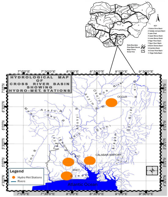
Figure 1.
Hydrological Map of the Cross River Basin showing the Hydromet Stations. The insert at the top right is the map of Nigeria adopted from Akpabio et al. [26].
The Cross River Basin is bound between latitudes 4°00′ N and 6°50′ N and longitudes 7°40′ E and 9°40′ E [27]. Typically, it has a tropical wet climate with high rainfall (between 1250 mm and 4000 mm annually), high temperatures (between 22 °C and 30 °C), and high relative humidity. Agriculture is the main economic activity in the basin.
According to Okoji [28], most of the dwellers in the Cross River Basin depend mostly on agricultural activities such as the production of food and cash crops, animal husbandry, the cultivation of plants for medicine and ornamental plants to maintain green areas, and the aesthetics of the catchment especially in Calabar. These underscored the need for the establishment of the CRBDA.
The records of the primary (climatic) data used in this study were generated by the Nigerian Meteorological Agency (NiMet), a federal government establishment tasked with the responsibility of recording, collating, processing, and disseminating meteorological data in Nigeria for research activities and to guide policy making. The meteorological data for the Cross River Basin catchment were recorded and processed through four gauge stations located in Uyo, Calabar, Eket, and Ogoja. The Cross River Basin is located in Southeast Nigeria near the southwestern border of Cameroon. A major feature of this basin is Cross River which originates from Cameroon passing through Nigeria as it empties into the Atlantic Ocean. The monthly and yearly records of climatic variables from 1992 to 2021 were obtained from Uyo, Calabar, Eket, and Ogoja gauge stations. The climatic variables studied were atmospheric temperature, soil temperature, humidity, rainfall, sunlight hours, evaporation, wind speed, cloud cover, solar radiation, and atmospheric pressure.
Records of the average values of climatic variables for each month and year from 1992 to 2021 were obtained from the Nigerian Meteorological Agency (NiMet). These were based on observations at four gauge stations located in Ogoja, Calabar, Uyo, and Eket (Table 1). All the datasets were consistent, with no gaps in records. The datasets comprised annual average rainfall, maximum and minimum temperatures, humidity, duration of sunlight (sunshine hours), evaporation, wind speed, soil temperature, cloud cover, solar radiation, and atmospheric pressure for 30 years.

Table 1.
Location of the weather stations.
The ENSO data used for the analysis are given as the El Nino Southern Oscillation Indices (SOIs), which were derived by the National Centers for Environmental Information [29] using standardized values of sea level pressures in Tahiti and Darwin, Australia (Equation (6)). These were derived for each month from 1992 to 2021. Table 1 provides relevant information from the hydro-meteorological stations. The table contains the station name, local government area (LGA), state, and geographical coordinates.
2.2. Methods
The MK test, along with linear variations in the data represented by Kendall–Theil robust lines, was used to detect the long-term trends observed in the time series data collected from four hydro-meteorological stations in the basin. Fluctuations in the hydro-meteorological regimes were assessed using the non-parametric MK test, which is best suited for evaluating hydrologic changes [30]. In this study, trend analysis was carried out to examine the presence of a trend (downward or upward) or the absence of a trend.
2.2.1. Mann–Kendall Trend Detection
To detect trends in hydro-meteorological time series data, especially in a scenario where data points are normally distributed, the Mann–Kendall (MK) test, which is a non-parametric test, is generally used [31,32]. It is best suited for distribution-free data where no pre-assumption of the data is made. This conditionality contrasts with the parametric tests in which assumptions are made regarding the distribution of data before they are analyzed (for instance, if the data are normally distributed). Non-parametric tests are applicable where the distribution of the data is not clearly defined or immediately known, especially where there is no serial correlation between the variables.
The MK test is also used for the identification of trends in several other fields of study like medicine, hydrology, climatology, and environmental sciences [33,34,35,36]. In our case, trends in hydro-meteorological data can be detected with the use of the MK test. Therefore, in this study, the MK test was applied for the detection of trends in the observed data for annual average rainfall, maximum and minimum temperatures, humidity, solar radiation, duration of sunlight, atmospheric pressure, evaporation, wind speed, runoff, soil temperature, and cloud cover.
To determine the Mann–Kendall statistics, the following expressions were applied:
where = annual values in years j and k, respectively, and j > k.
An increase in trend was identified when the statistic (S) had a high positive value, while a decrease in trend was identified when there was a low negative value. However, in achieving the statistical quantification of the significance levels in the observed trends, the calculation of the probability (p) of having the statistic (S) with the sample size (n) is very important [37]. Thus, Equation (3), given below, was applied in calculating the variance of S:
where q = the number of tied groups and = the number of data values in the tied group. Here, a collection of data points with the same values is called a tied group. By applying Equation (4) below, the test statistic (Z) was computed with VAR(S) and S values:
At the 5% level, (Z0.025 = 1.96), the value of Z was tested.
This study was designed to evaluate the hypothesis that there is no trend in the magnitude of climatic parameters over time. Here, the sample size, n, is the average annual rainfall depth for 30 years, calculated from the daily records. The null hypothesis (H0) would be rejected if the value obtained for p was less than the significance limit (α = 0.05). The rejection of H0 indicated the existence of a trend, while the acceptance of H0 indicated the non-existence of a trend. The result was statistically significant if H0 was rejected. The R-Studio 4.3.4 software was used to carry out these computations.
2.2.2. Illustrating the Mann–Kendall Analysis
The process of the Mann–Kendall analysis is best demonstrated using a given set of data. The average annual rainfall record is considered in this case and is used to describe the application of the approach. The records of the average annual rainfall spanning 30 years were obtained from the Calabar meteorological station and Cross River State from 1992 to 2021 and used for the statistical analysis. The following processes were applied.
The Mann–Kendall statistic (S) was determined from Equation (1). It is worth noting that, at this stage, a comparison of the relative magnitude of data entries was made instead of the actual numeric data values. The dataset was treated as an ordered time series, where each successive value was compared to its predecessors. S values were either 0, 1, or −1, and an initial value of 0 was assumed at the start of the calculation. For the range of average annual rainfall data and by applying Equations (1) and (2), S was determined as −277. The variance of S, VAR (S), was calculated through Equation (3), where the sample size (n) was 30, the number of tied groups (q) was 0, and the number of data values in the tied group () was also 0. VAR (S) was determined as 3141.67.
The formulation for the Mann–Kendall normalized test statistic () is dependent on the status of S, as defined in Equation (4). In this case, is calculated as −4.924. At a 5% level of testing (corresponding to a significant limit, ), the z score for a normal distribution is given as 1.96. ; therefore, the null hypothesis () is rejected. The calculated corresponds to a p-value = 0, which confirms the decision to reject .
2.2.3. Modified Mann–Kendall Trend Detection
A modified Mann–Kendall analysis was also performed to account for the effects of autocorrelations in the time series data. Detailed information on this method is presented in Hamed and Rao [4]. The modified Mann–Kendall test is established principally by adjusting the variance of S, as given in Equations (5)–(7) [4].
where is the real number of observations, and is a correction to account for autocorrelation in the data, expressed as:
where is the effective number of observations when considering autocorrelation, and is the autocorrelation between the ranks of observations (rank correlation), which can be transformed into the normalized data autocorrelation by the following:
3. Results and Discussion
3.1. Analysis of Rainfall
Table 2 contains the descriptive statistics for rainfall in the Cross River Basin, which include the maximum and minimum values, and the mean, standard deviation, skewness, and kurtosis. The records of rainfall data were obtained from four stations (Eket, Uyo, Calabar, and Ogoja). The descriptive statistics for annual rainfall in the basin, as presented in Table 2, show that the minimum annual rainfall of 104.3 mm was recorded in Ogoja, while the highest maximum annual rainfall of 7094.3 mm was observed in Calabar. Consequently, the highest mean annual rainfall was 4454.3 mm in Calabar, and the lowest mean annual rainfall was 196.9 mm in Ogoja. In other words, the maximum value of annual rainfall was the highest maximum annual rainfall of 7094.3 mm, which was observed at Calabar station, while the highest mean annual rainfall of 4454.3 mm was observed at Calabar station.

Table 2.
Results of Descriptive Statistics for Rainfall in Cross River Basin from 1992 to 2021.
The variability was also highest in Calabar, with a standard deviation of 1495.442. The annual rainfall was positively skewed in the entire basin, while kurtosis was negative for Calabar and Ogoja. The trend analysis using the Mann–Kendall test for rainfall in the basin (Table 3) showed that the null hypothesis H0 was accepted for Eket and Uyo (i.e., p-value > 0.05), meaning that there is no significant trend in rainfall in Eket and Uyo, whereas H0 was rejected (p-value < 0.05) for Ogoja, showing a significant upward trend in rainfall, and for Calabar, showing a significant downward trend in rainfall. This is supported by the corresponding Kendall Tau coefficients. In Eket and Uyo, there is no correlation between the magnitudes of rainfall data and time (), which is also observed in Figure 2, where there is no clear pattern in rainfall data across the gauge stations in Eket and Uyo.

Table 3.
Results of Mann–Kendall Test for Rainfall from 1992 to 2021.
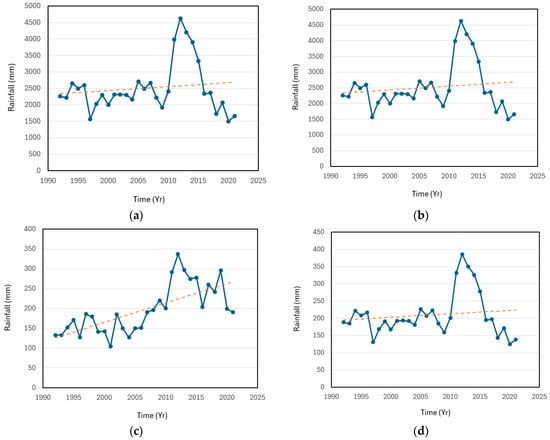
Figure 2.
Trends of rainfall for the Cross River Basin catchment: (a) Temporal variability and linear trend in rainfall in Calabar. Linear trend model Yt = 6734.818 − 147.1284 t; (b) Temporal variability and linear trend in rainfall in Uyo. Linear trend model Yt = 2322.608 + 12.036 t; (c) Temporal variability and linear trend in rainfall in Ogoja. Linear trend model Yt = 121.103 + 4.888 t; and (d) Temporal variability and linear trend in rainfall in Eket. Linear trend model Yt = 193.552 + 1.003 t. The linear trends are shown by the dotted lines.
Contrarily, the Kendall Tau coefficients for Calabar () and Ogoja () indicate strong correlations with time, and the corresponding patterns are depicted in Figure 2. The trend analysis of rainfall in the basin shows a significant upward trend only in Ogoja, while in Calabar, there is a downward trend. The S statistic was observed to be highest in Ogoja. The rainfall trend in the Cross River Basin is increasing only in Ogoja, with the highest trend rate of 4.517 (Figure 2), while Calabar is recording a significant decrease in rainfall.
The significant upward trend in rainfall in Ogoja has a significant impact on the hydrology of the area. The trend is in accordance with investigations carried out by Ogunrinde et al. [38] with respect to the changes in the indices of rainfall and drought in Nigeria from 1981 to 2015, where a general rise in trend in rainfall was observed across the country. This rise in rainfall trend at Ogoja station and its surroundings had a causal effect that led to the recent 2022 flood disaster that occurred in the area, resulting in the overflow of Cross River along its banks and the complete submergence of the Ogoja–Ikom–Calabar Federal Highway over seven (7) days at the Ikom (Okuni) section of the road. The results also confirm the findings from the analysis of the trends in climatic variables in Southeast Nigeria and the Kanji Lake Basin, conducted by Osugiri et al. [39] and Salami et al. [40], respectively. Both findings indicate an upward trend in rainfall intensity that is significant at p = 0.01. Salami et al. [40] also revealed an upward trend in maximum temperature and evaporation. However, as shown in Calabar, a rise in rainfall is not always observed. In the Cross River Basin, Calabar exhibited a statistically significant negative (decreasing) trend in rainfall. This is consistent with records from other studies, e.g., Zitta and Madaki [41], Tarek et al. [42] and Ozi-Isah et al. [43].
Zitta and Madaki [41] revealed a unimodal and downward trend in rainfall in Jos over a 30-year period using rainfall anomaly index (RAI), analysis of variance, and a 5-year moving average. In this region, the mean rainfall was recorded as 1326.3 mm, with variability consistent at 400 mm.
Tarek et al. [42] observed a significant decrease in rainfall in Sharjah City, UAE, while the same trend was noted by Ozi-Isah et al. [43] in the Niger and Benue confluence catchments in Lokoja, Kogi State, Nigeria. In the confluence area, there was an average decrease of about 462.7 mm.
The decreasing depth of rainfall in Calabar is instrumental to the recent reduction in runoff and flooding in the region and its surroundings.
3.2. Analysis of Evaporation
An analysis of the descriptive statistics for annual evaporation in the basin, as presented in Table 4, reveals that the minimum annual evaporation of 1.9 mm was recorded in Eket, while the highest maximum annual evaporation of 2.9 mm was observed in Calabar. Consequently, the highest mean annual evaporation was 2.6 mm in Calabar. The lowest mean annual evaporation was 2.2 mm in Uyo, while the annual evaporation in Eket was the most variable, with a standard deviation of 0.156 mm. In Calabar and Ogoja, the annual evaporation was positively skewed, whereas in Eket and Uyo, the skewness was negative. This indicates that in Calabar and Ogoja, a wider range of data values was higher than the mean annual evaporation. On the other hand, in Eket and Uyo, a wider range of data values was below the mean annual evaporation. Only Uyo had a negative kurtosis. Higher evaporation values in Calabar also influenced the decrease in runoff at the station. Despite having lower rainfall depths, the annual evaporation recorded at Ogoja station is in the same range as those in Calabar (Figure 2 and Figure 3). Consequently, the runoff observed at Ogoja station is low (Figure 4). This indicates a relationship between runoff and evaporation.

Table 4.
Results of Descriptive Statistics for Evaporation from 1992 to 2021.
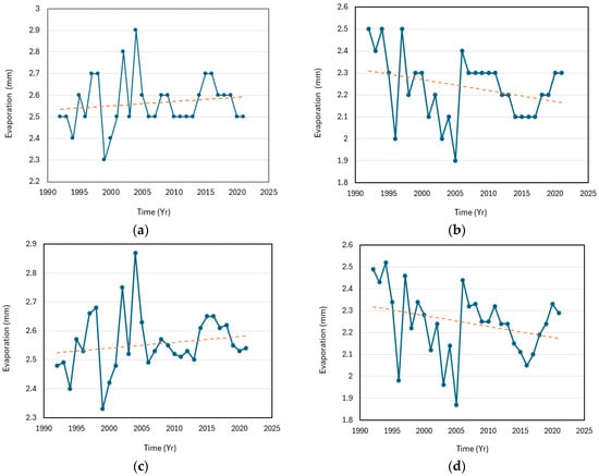
Figure 3.
Trends of evaporation for the Cross River Basin catchment: (a) Temporal variability and linear trend in evaporation in Calabar. Linear trend model Yt = 2.533 + 0.002 t; (b) Temporal variability and linear trend in evaporation in Uyo. Linear trend model Yt = 2.315 − 0.005 t; (c) Temporal variability and linear trend in evaporation in Ogoja. Linear trend model Yt = 2.522 + 0.002 t; and (d) Temporal variability and linear trend in evaporation in Eket. Linear trend model Yt = 2.323 − 0.005 t. The linear trends are shown by the dotted lines.
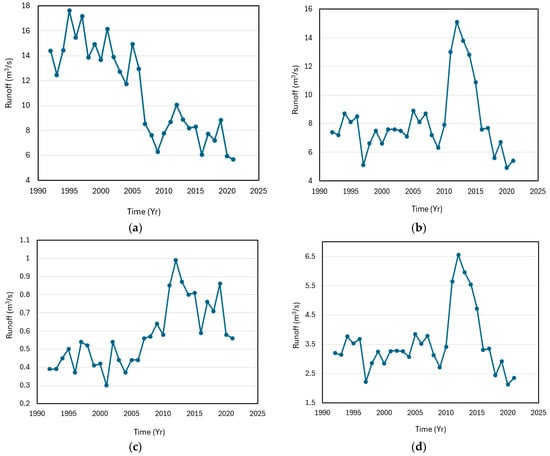
Figure 4.
Trends of runoff for Cross River Basin catchment: (a) Temporal variability of runoff in Calabar; (b) Temporal variability of runoff in Uyo; (c) Temporal variability of runoff in Ogoja; and (d) Temporal variability of runoff in Eket.
The Mann–Kendall evaporation test for the basin (Table 5) shows that the null hypothesis H0 with a p-value of 0.038 was rejected only in Eket, with a decreasing trend, and the null hypothesis H0 was accepted in the other three stations of the catchment, indicating that there is no significant trend in the other stations. The trend line in Figure 3 indicates momentary spikes in evaporation but an overall downward trend over the duration of observation (1990–2020). A downward trend in evaporation in certain areas of Nigeria is not unusual; for instance, the Mann–Kendall trend analysis conducted by Oguntunde et al. [44] showed a significant downward trend in evaporation at Ibadan. The decreasing trend in evaporation can be attributed to the rise in harmattan haze in that region, caused by climate change. At the other weather stations in the Cross River Basin, there is no significant trend in evaporation.

Table 5.
Results of Mann–Kendall Test for Evaporation (mm) from 1992 to 2021.
3.3. Analysis of Wind Speed
The descriptive statistical results for annual wind speed in the Cross River Basin catchment are shown in Table 6. The minimum annual wind speed in the catchment area, 2.8 knots, was recorded at Eket station, while the maximum annual wind speed, 5.8 knots, was recorded at Ogoja station. The highest mean annual wind speed of 4.3 knots was observed in Calabar, whereas the lowest mean annual wind speed of 3.7 knots was obtained in Eket. From the data analysis, the annual wind speed in Uyo was the most variable, with a standard deviation of 0.785. It was only in Calabar that the annual wind speed was negatively skewed. The skewness values of annual wind speed in Eket, Uyo, and Ogoja were positive. Kurtosis was negative in the entire basin/catchment.

Table 6.
Results of Descriptive Statistics for Wind Speed from 1992 to 2021.
From the Mann–Kendall test for wind speed (Table 7), the null hypothesis H0 was rejected in the basin, except for Ogoja, where the null hypothesis H0 was accepted in the catchment. This analysis shows that there is a significant rising trend in the wind speed in the Cross River Basin. This significant increasing trend in wind speed agrees with the findings from the Mann–Kendall statistical analysis performed by Solomon and Sunday [45], which demonstrated a significant upward trend in wind speed across nine stations in Nigeria. In the Uyo and Eket regions, there is a significant rise in the trend in wind speed, unlike in Calabar, where there is a downward trend, especially close to 2020 (Figure 5). The rapid decline in wind speed in Calabar shortly before 2020 deviates from the general pattern from previous years and is likely to have an impact on the overall results for that area.

Table 7.
Results of Mann–Kendall Test for Wind Speed from 1992 to 2021.

Figure 5.
Trends of wind speed for the Cross River Basin catchment: (a) Temporal variability and linear trend in wind speed in Calabar. Linear trend model Yt = 4.814 − 0.033 t; (b) Temporal variability and linear trend in wind speed in Uyo. Linear trend model Yt = 2.726 + 0.065 t; (c) Temporal variability and linear trend in wind speed in Ogoja. Linear trend model Yt = 4.298 − 0.005 t; and (d) Temporal variability and linear trend in wind speed in Eket. Linear trend model Yt = 2.782 + 0.059 t. The linear trends are shown by the dotted lines.
3.4. Analysis of Solar Radiation
Table 8 shows the analysis of descriptive statistics for solar radiation in the Cross River Basin. From the analysis, the minimum annual solar radiation of 15.9 mj/m2/year was observed in Calabar, while the maximum annual solar radiation was 20.5 mj/m2/year in Ogoja. Also, the highest mean annual solar radiation was 18.9 mj/m2/year in Ogoja, and the lowest was 17.5 mj/m2/year in Calabar. The highest mean annual solar radiation recorded in Ogoja is consistent with the highest number of hours of sunshine, which was also observed in Ogoja. The annual solar radiation in Calabar was the most variable, with a standard deviation of 1.1 mj/m2/year. The annual solar radiation was only positively skewed in Calabar, and kurtosis was negative in Calabar and Ogoja.

Table 8.
Results of Descriptive Statistics for Solar Radiation from 1992 to 2021.
In Table 9, the Man-Kendall test for solar radiation shows that the null hypothesis H0 was accepted in all stations except Calabar, which had a p-value of 0.041, showing a significant upward trend in solar radiation. The S statistic was observed to be highest in Calabar; this also explains why Calabar recorded the most significant pattern (upward increase) in the entire basin. The solar radiation trend (Figure 6) is rising at Calabar station, while there is no significant trend at all the other stations in the catchment. Also, for the period of study, the highest solar radiation trend intensity occurred in Calabar (0.06 mj/m2/year). The increase in solar radiation at Calabar station agrees with the findings from the trend analysis performed by Ogolo [46] using a modified Angstrom model. The investigation by Ogolo [46] showed a significant upward trend in solar radiation in Nigeria.

Table 9.
Results of Mann–Kendall Test for Solar Radiation from 1992 to 2021.
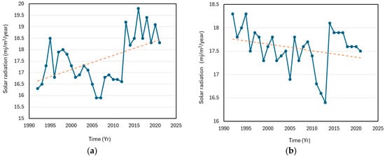
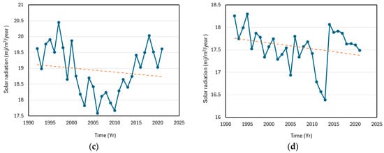
Figure 6.
Trends of solar radiation for Cross River Basin catchment: (a) Temporal variability and linear trend in solar radiation in Calabar. Linear trend model Yt = 16.573 + 0.062 t; (b) Temporal variability and linear trend in solar radiation in Uyo. Linear trend model Yt = 17.778 − 0.014 t; (c) Temporal variability and linear trend solar radiation in Ogoja. Linear trend model Yt = 19.129 − 0.013 t; and (d) Temporal variability and linear trend in solar radiation in Eket. Linear trend model Yt = 17.772 − 0.013 t. The linear trends are shown by the dotted lines.
The increase in solar radiation is in line with increasing annual average temperatures and is consistent with the evidence of climate change at both regional and global scales.
3.5. Analysis of Sunshine Hours
The analysis for the descriptive statistical results for sunshine hours in the Cross River Basin is shown in Table 10. The minimum value of sunshine hours was 2.1, recorded in Uyo, while the maximum value of 6.5 hours was observed in Ogoja. The highest mean annual sunshine was 5.8 h, recorded in Ogoja, while the lowest mean annual sunshine hours of 3.5 h was in Eket. The highest mean value of sunshine hours recorded in Ogoja is consistent with those generally observed in the northern parts of Nigeria due to its proximity to those areas.

Table 10.
Results of Descriptive Statistics for Sunshine from 1992 to 2021.
The annual sunshine in Uyo was the most variable, with a standard deviation of 0.827. It was only in Calabar that the annual sunshine was positively skewed. Kurtosis was negative in the entire basin.
The test results of the Mann–Kendall analysis for sunshine hours are given in Table 11. Based on the analysis, the null hypothesis H0 was accepted in all the stations except for Calabar. Therefore, it means that there is no defining trend in sunshine hours in Eket, Uyo, and Ogoja. The only significant decrease in trend is in Calabar. The S statistic was observed to be positive and highest in Eket, which suggests a generally increasing trend in sunshine hours; however, this trend is considered to be statistically insignificant at the 5% level of testing. The patterns observed in Uyo and Ogoja are also statistically insignificant. Hence, across the basin (Figure 7), the trend in sunshine hours is decreasing in Calabar, while those recorded from the other stations in the catchment are statistically insignificant. The decrease in sunshine hours observed in Calabar is not an isolated incidence and is consistent with the records of some other basins in Nigeria, such as those reported by Amadi et al. [47], where a linear regression model was used to determine the trend in the duration of sunshine hours between 1961 and 2012. Amadi et al. [47] detected a decline in sunshine hours in seven stations in Nigeria, namely, Sokoto, Kaduna, Bauchi, Maiduguri, Yola, Lokoja, and Ogoja. The outcome of this study, supported by reports of other investigations (e.g., [47]), lends credence to increasing concerns about the potential impact of anthropogenic aerosol emissions on the dynamics of atmospheric circulations at synoptic scales.

Table 11.
Results of Mann–Kendall Test for Sunshine Hours from 1992 to 2021.
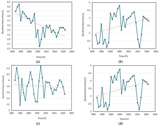
Figure 7.
Trends of sunshine hours for the Cross River Basin catchment: (a) Temporal variability and linear trend in sunshine hours in Calabar. Linear trend model Yt = 4.035 − 0.034 t; (b) Temporal variability and linear trend in sunshine hours in Uyo. Linear trend model Yt = 2.992 + 0.033 t; (c) Temporal variability and linear trend in sunshine hours in Ogoja. Linear trend model Yt = 5.868 − 0.004 t; and (d) Temporal variability and linear trend in sunshine hours in Eket. Linear trend model Yt = 2.981 + 0.033 t. The linear trends are shown by the dotted lines.
3.6. Analysis of Atmospheric Pressure
The analysis of atmospheric pressure is presented in Table 12. The minimum value of atmospheric pressure of 1010.8 millibars was recorded in Calabar and Ogoja, while the maximum value of 1015.4 millibars was recorded in Eket. The highest value of mean annual atmospheric pressure in the catchment was 1014.9 millibars, observed in Uyo, while the lowest value of mean annual atmospheric pressure was 1011.8 millibars and observed at Ogoja. The variability was highest in Eket, with a standard deviation of 0.877. It was only in Uyo that the annual atmospheric pressure was positively skewed. Kurtosis was negative in Calabar and Ogoja. From the Mann–Kendall analysis of the data for atmospheric pressure in the basin, the null hypothesis H0 was accepted for all stations in the catchment except Eket, which had the only significant upward trend (Table 13). The S statistic was observed to be highest in Calabar. The atmospheric pressure in the Cross River Basin is increasing in Eket, where the highest rate (0.018) was also recorded (Figure 8). The rise in atmospheric pressure is similar to occurrences in other regions of Nigeria. For example, in Ikogosi, Ogun State (Southwest Nigeria), there is an exponential rise in atmospheric pressure, which is considered to be indicative of climate change [48].

Table 12.
Results of Descriptive Statistics for Atmospheric Pressure from 1992 to 2021.

Table 13.
Results of Mann–Kendall Test for Atmospheric Pressure from 1992 to 2021.
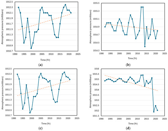
Figure 8.
Trends of atmospheric pressure for the Cross River Basin catchment: (a) Temporal variability and linear trend in atmospheric pressure in Calabar. Linear trend model Yt = 1011.456 + 0.020 t; (b) Temporal variability and linear trend in atmospheric pressure in Uyo. Linear trend model Yt = 1014.974 − 0.005 t; (c) Temporal variability and linear trend in atmospheric pressure in Ogoja. Linear trend model Yt = 1011.447 + 0.020 t; and (d) Temporal variability and linear trend in atmospheric pressure in Eket. Linear trend model Yt = 1015.427 − 0.051 t. The linear trends are shown by the dotted lines.
3.7. Analysis of Maximum Temperature
Table 14 shows the descriptive statistics of annual maximum temperatures for the basin. The minimum annual maximum temperature was 30.2 °C, recorded in Calabar, while the highest annual maximum temperature of 33.8 °C was recorded in Ogoja. The highest mean annual maximum temperature of 32.3 °C was observed in Ogoja, while the lowest mean annual maximum temperature of 31 °C was observed in Calabar. The maximum temperature was negatively skewed in the entire basin. Kurtosis was positive in Eket and Uyo but negative in Calabar and Ogoja. The occurrence of the highest mean annual maximum temperature in Ogoja can be attributed to its proximity to the northern part of the country, which has traditional semi-arid conditions and a history of high mean temperatures. It confirms the effects of climate change marked by a continuing rise in temperatures in regions closer to the desert, resulting in increased desertification. This analysis also agrees with results regarding sunshine hours, solar radiation, and soil temperature, where Ogoja had the highest values.

Table 14.
Results of Descriptive Statistics for Maximum Temperature from 1992 to 2021.
According to the Mann–Kendall analysis (Table 15), the null hypothesis H0 was rejected in the entire catchment except in Ogoja, which implies a statistically significant increase in temperatures in the other areas of the catchment (Calabar, Eket, and Uyo). The rising temperature in the catchment agrees with the worldwide observations of changes in climate due to rising temperatures. The analysis also showed a significant increase in temperatures. The S statistic was observed to be highest in Calabar. Figure 9 explains the rising trend in annual maximum temperatures on the basin scale, where there is a very significant upward trend in maximum temperatures in the Cross River Basin. This regional increase is in line with the global observations of the increase in temperatures due to climate change and the resolution since 1990, when the Intergovernmental Panel on Climate Change (IPCC) confirmed the increase in greenhouse gases in the atmosphere and the resulting global warming of the earth.

Table 15.
Results of Mann–Kendall Test for Maximum Temperature from 1992 to 2021.
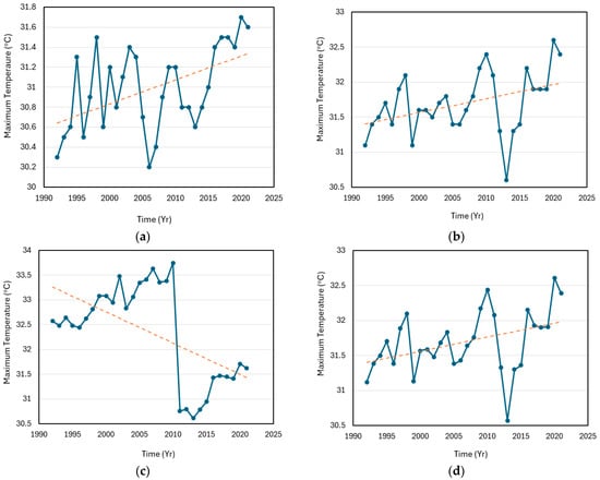
Figure 9.
Trends of maximum temperature for the Cross River Basin catchment: (a) Temporal variability and linear trend in maximum temperature in Calabar. Linear trend model Yt = 30.617 + 0.024 t; (b) Temporal variability and linear trend in maximum temperature in Uyo. Linear trend model Yt = 31.385 + 0.020 t; (c) Temporal variability and linear trend in maximum temperature in Ogoja. Linear trend model Yt = 33.325 − 0.063 t; and (d) Temporal variability and linear trend in maximum temperature in Eket. Linear trend model Yt = 31.382 + 0.020 t. The linear trends are shown by the dotted lines.
The rise in temperature conforms with the established trend in Akure, Southwest Nigeria based on the work by Ayeni and Oloukoi [49]. Ayeni and Oloukoi [49] investigated the change in temperature as an indicator of climate change using land surface temperature and meteorological data from Akure. They recognized an increase in the maximum, minimum, and average land surface temperatures within decades. For example, the land surface temperature increased from 26.4 °C in the base year (1990) to 27.2 °C, 27.3 °C, and 28.3 °C in the years 2000, 2010, and 2020, respectively. The outcome of these studies attests to the claims of climate change as well as the indices to measure its occurrence and severity, which can also serve as tools to aid the formulation of mitigating solutions to global warming. The highest trend rate was recorded in Calabar.
3.8. Analysis of Soil Temperature
Table 16 shows the descriptive statistics for soil temperature in the Cross River Basin. The minimum soil temperature was recorded in Calabar, and the maximum soil temperature, 29.4 °C, was recorded in Eket. The highest mean annual soil temperature was observed in Uyo, with a value of 28.9 °C, while the lowest value, 27.6 °C, was recorded in Calabar. The annual soil temperature in Calabar was the most variable, with a standard deviation of 0.852. The kurtosis and skewness of annual soil temperature were negative in the entire catchment. Based on the Mann–Kendall analysis (Table 17), the null hypothesis H0 was accepted in the entire catchment, which shows that there is no significant trend in soil temperature in the Cross River Basin. The outcome of the analysis is also reflected in Figure 10, where regular fluctuation in temperatures is exhibited across the four stations in the catchment area. This result agrees with those from other parts of the world, such as Iran, where no significant trend in soil surface temperature was observed for all the time series based on the research by Nozar et al. [50] using regression analysis.

Table 16.
Results of Descriptive Statistics for Soil Temperature from 1992 to 2021.

Table 17.
Results of Mann–Kendall Test for Soil Temperature from 1992 to 2021.
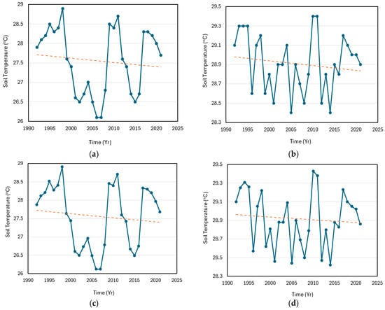
Figure 10.
Trends of soil temperature for the Cross River Basin catchment: (a) Temporal variability and linear trend in soil temperature in Calabar. Linear trend model Yt = 27.721 − 0.011 t; (b) Temporal variability and linear trend in soil temperature in Uyo. Linear trend model Yt = 28.984 − 0.005 t; (c) Temporal variability and linear trend in soil temperature in Ogoja. Linear trend model Yt = 27.731 − 0.011 t; and (d) Temporal variability and linear trend in soil temperature in Eket. Linear trend model Yt = 28.964 − 0.003 t. The linear trends are shown by the dotted lines.
3.9. Analysis of Cloud Cover
Table 18 shows the descriptive statistics for cloud cover in the Cross River Basin catchment. The minimum (6.0) and maximum (10.0) annual cloud cover values were recorded in Eket. The highest mean annual cloud cover (7.0) was recorded in Uyo, Calabar, and Ogoja, whereas the lowest mean annual cloud cover (6.733) was recorded in Eket. The annual cloud cover in Eket was the most variable, with a standard deviation of 0.785. In Eket, the kurtosis and skewness of annual cloud cover were positive. According to the Mann–Kendall analysis for cloud cover (Table 19), the null hypothesis H0 was accepted in the entire basin. Therefore, this observation implies that there is no significant trend in cloud cover across the Cross River Basin.

Table 18.
Results of Descriptive Statistics for Cloud Cover (Oktas) from 1992 to 2021.

Table 19.
Result of Mann–Kendall Test for Cloud Cover from 1992 to 2021.
3.10. Analysis of Relative Humidity
The descriptive statistics and patterns for relative humidity in the Cross River Basin are given in Table 20 and Figure 11, respectively. The minimum annual relative humidity (68.6%) was recorded in Ogoja, while the maximum value (92%) was recorded in Uyo. The highest mean annual relative humidity was 85.2% in Calabar, whereas Ogoja had the lowest value of 72.4%. The result also shows that the annual relative humidity in Eket was the most variable, with a standard deviation of 5.627. The annual relative humidity was positively skewed in the entire basin. Likewise, kurtosis was positive in the basin.

Table 20.
Results of Descriptive Statistics for Relative Humidity (%) from 1992 to 2021.
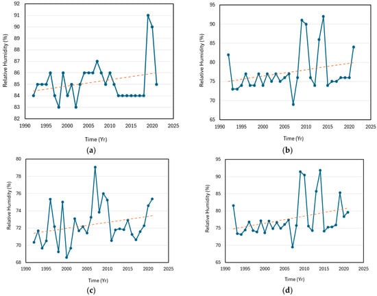
Figure 11.
Trends of relative humidity for the Cross River Basin catchment: (a) Temporal variability and linear trend in relative humidity in Calabar. Linear trend model Yt = 84.352 + 0.055 t; (b) Temporal variability and linear trend in relative humidity in Uyo. Linear trend model Yt = 74.890 + 0.168 t; (c) Temporal variability and linear trend in relative humidity in Ogoja. Linear trend model Yt = 71.334 + 0.070 t; and (d) Temporal variability and linear trend in relative humidity in Eket. Linear trend model Yt = 74.587 + 0.207 t. The linear trends are shown by the dotted lines.
Based on the Mann–Kendall analysis, the null hypothesis H0 was accepted for all the stations in the Cross River Basin except Eket, where the null hypothesis H0 was rejected with a p-value of 0.045, revealing a significant increasing trend in relative humidity in Eket (Table 21). The lack of a statistically significant trend in most sections of the Cross River Basin supports the results from previous investigations conducted within the same geographical area. An instance of this is the assessment of variations in relative humidity in Calabar, Nigeria, completed by Osang et al. [51]. Osang et al. [51] provides an account of increasingly high relative humidity in Calabar and other tropical rainforest areas, with no clear trend between 2003 and 2012. However, for each year, the highest relative humidity tends to occur between July and August. On the other hand, the lowest relative humidity normally occurs in January.

Table 21.
Result of Mann–Kendall Test for Relative Humidity from 1992 to 2021.
3.11. The Influence of Autocorrelation
It is expedient to also conduct a modified Mann–Kendall test to incorporate the effect of autocorrelations in the time series data. The details of this method are explained in Hamed and Rao [4]. Autocorrelation exists if a range of variables and its lagged version are correlated across various time intervals. This is important because the presence of either a positive or negative autocorrelation in time series, while not affecting the outcome of the test, can influence the ability to distinguish between a significant and non-significant trend. In this study, the results from the modified Mann–Kendall test do not deviate considerably from those produced when autocorrelation is not considered. Any difference is marginal and validates the trend detections presented earlier. These are presented in Table 22, Table 23, Table 24 and Table 25.

Table 22.
Modified Mann–Kendall’s test results for Calabar.

Table 23.
Modified Mann–Kendall’s test results for Uyo.

Table 24.
Modified Mann–Kendall’s test results for Eket.

Table 25.
Modified Mann–Kendall’s test results for Ogoja.
In Calabar, the Z-values for variables like runoff, rainfall, maximum temperature, minimum temperature, solar radiation, sunshine hours, and wind speed are large (either significantly negative or positive). This indicates that these variables’ trends are strong and fall within the tails of the empirical bootstrapped distribution, implying a significant departure from the null hypothesis. Therefore, there is likely a trend in these variables. Conversely, for variables like relative humidity, atmospheric pressure, soil temperature, and evaporation, the Z-values are smaller and closer to zero. These values suggest that the trends for these variables are not strong and may not significantly deviate from what would be expected under the null hypothesis. Therefore, there may not be a trend in these variables, and if there is, it is not statistically significant.
In Uyo, the Z-values for maximum temperature and wind speed in the Akwa Ibom region, are relatively large and fall within the tails of the empirical bootstrapped distribution. For maximum temperature, the Z-value is 2.3511, while for wind speed, it is 4.0176. These high Z-values suggest significant departures from the null hypothesis of no trend, indicating the presence of trends in these variables. On the other hand, variables like runoff, rainfall, solar radiation, sunshine hours, relative humidity, atmospheric pressure, soil temperature, and evaporation have smaller Z-values that are closer to zero. They do not fall within the tails of the empirical bootstrapped distribution, implying that these variables do not exhibit significant departures from the null hypothesis. Therefore, there may not be any trend in these variables, and if there are, they are not statistically significant.
In Eket, the Z-values for maximum temperature, relative humidity, wind speed, atmospheric pressure, and evaporation are relatively large and fall within the tails of the empirical bootstrapped distribution. The Z-values are 2.3028 for maximum temperature, 1.9982 for relative humidity, 3.7663 for wind speed, −1.9813 for atmospheric pressure, and −2.0737 for evaporation. These Z-values suggest significant departures from the null hypothesis of no trend, indicating the presence of trends in these variables. Conversely, for variables like runoff, rainfall, solar radiation, sunshine hours, minimum temperature, and soil temperature, the Z-values are smaller and closer to zero. They do not fall within the tails of the empirical bootstrapped distribution, implying that these variables do not exhibit significant departures from the null hypothesis. Therefore, there may not be trends in these variables, and if there are, they are not statistically significant.
For variables like runoff and rainfall in the Ogoja region, the Z-values are relatively large and fall within the tails of the empirical bootstrapped distribution. For runoff, the Z-value is 4.1448, and for rainfall, it is 4.1391. These high Z-values suggest significant departures from the null hypothesis of no trend, indicating the presence of trends in these variables. For other variables like minimum temperature, relative humidity, and atmospheric pressure, the Z-values are not as large as those for runoff and rainfall. Nonetheless, they are still beyond what would be expected under the null hypothesis. This means that there may be trends in these variables as well, even though they might not be as strong or significant as those observed for runoff and rainfall. Conversely, for variables like maximum temperature, solar radiation, sunshine hours, wind speed, soil temperature, and evaporation, the Z-values are smaller and do not fall within the tails of the empirical bootstrapped distribution. Hence, there may not be significant departures from the null hypothesis in these variables, denoting the absence of trends or weak trends that are not statistically significant.
4. Further Analyses and Discussion
4.1. El Nino Southern Oscillation (ENSO) Analysis
Serial correlation and segmented regression analyses were performed to measure the impact of fluctuations in monthly and long-term Tahiti and Darwin’s sea level pressures on the climatic variables in the Cross River Basin catchment. This additional set of analyses was necessary to determine the extent of the influence of the El Nino Southern Oscillation climatic cycle. The data of actual Tahiti and Darwin’s Sea level pressures (monthly and long-term average values) were used to calculate the El Nino Southern Oscillation Index (SOI) through Equation (5) [29,52]. The SOI data used in this study were derived from the National Centers for Environmental Information [29] using standardized values of sea level pressures in Tahiti and Darwin, Australia (Equations (8)–(13)).
where
- —El Nino–Southern Oscillation (ENSO) index;
- —Monthly sea level pressure in Tahiti;
- —Monthly sea level pressure in Darwin;
- —Mean monthly sea level pressure in Tahiti;
- —Mean monthly sea level pressure in Darwin;
- —Standard deviation of monthly sea level pressure in Tahiti;
- —Standard deviation of monthly sea level pressure in Darwin;
- —Standard deviation of standardized monthly sea level pressures;
- —Standardized monthly sea level pressure in Tahiti;
- —Standardized monthly sea level pressure in Darwin; and
- —Number of months.
4.1.1. Correlation Analyses and Dynamic Slopes of Segmented Regression
Correlation analyses were conducted to determine the dependencies between SOIs and various climatic variables for each month from 1992 to 2021. Four sets of climatic variables were examined: rainfall in Eket, rainfall in Ogoja, runoff in Eket, and runoff in Ogoja. Rainfall and runoff were studied because both are major indicators of changes in climatic conditions. The trend in correlations is necessary to determine the influence of ENSO events on the hydrological status of the Cross River Basin. Pearson’s correlation was calculated as per the following expression:
where is the Pearson’s correlation coefficient between SOI and the monthly magnitudes of the climatic variables for the month, ; and are the monthly SOI and magnitude of the climatic variables, respectively, for the month, , and the year, ; and and are the mean monthly SOI and magnitude of the climatic variables, respectively, for the month, , and the year, . Figure 12, Figure 13, Figure 14 and Figure 15 show the monthly correlation coefficients between the SOI and rainfall in Eket, rainfall in Ogoja, runoff in Eket, and runoff in Ogoja.
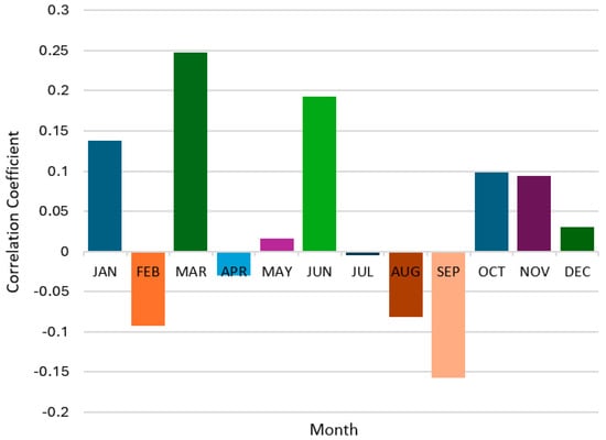
Figure 12.
Correlation coefficients between SOI and rainfall for Eket station from 1992 to 2021.

Figure 13.
Correlation coefficients between SOI and rainfall for Ogoja station from 1992 to 2021.
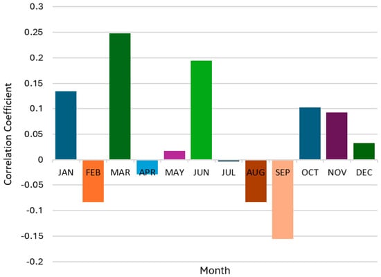
Figure 14.
Correlation coefficients between SOI and runoff for Eket station from 1992 to 2021.
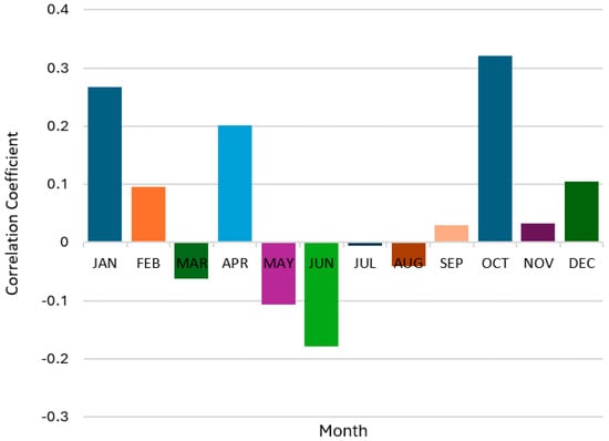
Figure 15.
Correlation coefficients between SOI and runoff for Ogoja station from 1992 to 2021.
The correlations between the SOI and the climatic variables (i.e., rainfall and runoff) are not consistent throughout the year. There are positive correlations in some months, while others are negative. In Eket, correlations between the SOI and rainfall as well as between the SOI and runoff are positive in January, March, May to June, and October to December, whereas they are negative in February, April, and July to September (Figure 12 and Figure 13). In Ogoja, correlations between the SOI and rainfall are positive in January to February, April, and October to December, but negative in March and May to August (Figure 14). In the same area, correlations between the SOI and runoff are positive in January, March, May, June, and October to December, whereas they are negative in the months of February, April, and July to September (Figure 15).
Furthermore, the impact of the ENSO on rainfall in the Cross River Basin catchment is not substantial. Correlations between the SOI and rainfall in Eket and Ogoja are weak overall. In Eket, the coefficient of correlation ranges from 0.005 in July to 0.248 in March, while in Ogoja, its lowest and maximum values are −0.006 in July and 0.321 in October, respectively. Therefore, according to the analysis, there is no significant association between the ENSO and rainfall in the catchment. It also implies that other factors are likely to influence rainfall characteristics and hence, the relationship between rainfall and ENSO events. In the same manner, the impact of the ENSO on runoff in the Cross River Basin catchment is not considerable. According to the regression analysis, the correlation coefficient between the SOI and runoff in Eket ranges from −0.004 in July to 0.248 in March, while the correlation between the SOI and runoff in Ogoja ranges from −0.006 in March to 0.321 in October. Thus, there is no significant association between the ENSO and runoff in the Cross River Basin. The range of p-values for all cases is less than 0.05 (); hence, the results are statistically significant at the 5% level of testing. However, additional analyses are still required to confirm these observations.
The slope of the regression line is then calculated as the dynamic slope of the segmented regression between the climatic variable (e.g., annual average monthly rainfall) and SOI and indicates the strength of the effect of the El Nino Southern Oscillation (ENSO) on the climatic variable—in this case, rainfall. The segmented regression is defined by Equation (8) [52,53], which is the dynamic slope of the regression line for a given year using the records of climatic data within and around the year under observation.
where
- —Slope of the regression line calculated for the year using records of climatic data from m years including and around the year;
- —Year under observation;
- —Number of years considered for the analysis;
- —Average monthly climatic variable (e.g., rainfall depth or runoff in year ); and
- —Average monthly in year
For each year investigated, three, seven, and nine years including and around the year were involved in the analysis (i.e., ). Dynamic slopes were computed for average monthly rainfall depth and runoff using the data from Eket and Ogoja gauge stations to determine the impact of ENSO events on the occurrences of both climatic variables. The rainy season is from April to October, and the dry season is from November to March. The results are presented in Figure 16, Figure 17, Figure 18 and Figure 19.
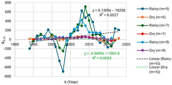
Figure 16.
Dynamic slopes from the segmented regression for m = 5, 7, and 9 for rainfall in Eket from 1992 to 2021.
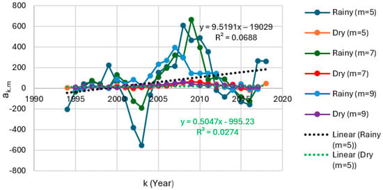
Figure 17.
Dynamic slopes from the segmented regression for m = 5, 7, and 9 for rainfall in Ogoja from 1992 to 2021.
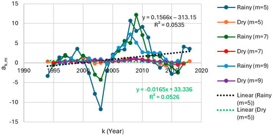
Figure 18.
Dynamic slopes from the segmented regression for m = 5, 7, and 9 for runoff in Eket from 1992 to 2021.
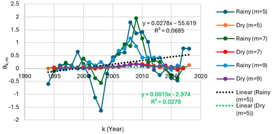
Figure 19.
Dynamic slopes from the segmented regression for m = 5, 7, and 9 for runoff in Ogoja from 1992 to 2021.
The dynamic slopes from the segmented regression for m = 5, 7, and 9 for rainfall in Eket during the rainy season are positive, indicating an increase in the effect of ENSO events on rainfall in successive years (i.e., from 1992 to 2021) (Figure 16). Contrarily, the dynamic slopes from the segmented regression for m = 5, 7, and 9 for rainfall in Eket during the dry season are negative, which shows a decrease in the impact of ENSO events on rainfall during the same period (Figure 16). A similar trend is observed in Ogoja for the rainy season. The dynamic slopes from the segmented regression for m = 5, 7, and 9 for rainfall in Ogoja during the rainy and dry seasons are positive. However, the dynamic slopes for the dry season are also positive, which show annual increases in the impact of ENSO events on rainfall during both seasons in Ogoja (Figure 17).
The trends in the dynamic slopes for runoff are akin to those observed for rainfall. The dynamic slopes from the segmented regression for m = 5, 7, and 9 for runoff in Eket are positive for the rainy season but negative for the dry season (Figure 18). These imply a general rise in the effect of ENSO events on runoff from 1992 through 2021 during the rainy season and a contrasting decline in the effect of ENSO events on runoff within the dry season across the same span of years. Likewise, the dynamic slopes from the segmented regression for m = 5, 7, and 9 for runoff in Ogoja are positive, considering the same range of rainy seasons, and negative for the corresponding set of dry seasons over the same duration in years. That is, they are negative when the focus is on the corresponding range of dry seasons over the course of the equivalent set of years (Figure 19). Hence, regarding runoff in Ogoja, there is an increase in the impact of ENSO events when rainy seasons are investigated, in contrast to a decrease in the effect of ENSO events during the dry seasons.
The trend lines (trends in ak,m) shown in Figure 16, Figure 17, Figure 18 and Figure 19 represent the linear regression for m = 5, and the slopes of these trend lines indicate the rate of increase or decrease in the impact of ENSO activities on climatic conditions. Other trend lines can be derived for m = 7 and m = 9 based on the respective set of ak,m values. The full range of slopes of trend lines for m = 5, 7, and 9 are defined in Table 26 for rainfall and Table 27 for runoff. In all cases, the slopes of trendlines for the rainy season are higher than for the dry season. Furthermore, the absolute values of the dynamic slopes for the rainy season are significantly higher in comparison with those for the dry season (Figure 16, Figure 17, Figure 18 and Figure 19), signifying a considerably greater impact of the attributes of the ENSO on rainfall and runoff during the rainy season for m = 5, 7, and 9. A similar pattern is shown when the slopes of trend lines for ak,m for rainy and dry seasons for m = 5, 7, and 9 are compared, reflecting much larger contributions from the ENSO in the rainy season.

Table 26.
Slopes of the linear regression models and their coefficients of determination for the dynamic slopes of the segmented regression lines for m = 5, 7, and 9 for rainfall from 1992 to 2021.

Table 27.
Slopes of the linear regression models and their coefficients of determination for the dynamic slopes of the segmented regression lines for m = 5, 7, and 9 for runoff from 1992 to 2021.
R2 is a measure of the goodness of fit of the linear regression model derived for each trend in the set of slopes of the segmented regression line. It is an indication, on a scale of 0 to 1, of how well the model fits the data and explains the changes in the slope of the segmented regression line (the dependent variable). Large values of R2 imply that there are small discrepancies between the actual data and the fitted model, whereas small values of R2 indicate the contrary. Because of the low R2 values observed in this study, the linear regression model for the range of slopes of the segmented regression line (dynamic slopes) is taken as a qualitative marker of the general trend in the 30-year period (1992–2021).
4.1.2. Intercepts of the Regression Lines Using Annual Average Monthly SOIs and Climatic Variables
In a similar manner to dynamic slopes, intercepts are also calculated from the segmented regression for the annual monthly SOIs and the associated annual monthly climatic variables. The series of intercepts is required to provide insights regarding the potential for the influence of other factors aside from ENSO events. The expression for the yearly intercepts, , is thus given as [52]:
where is the intercept of the regression line for the climatic variable, (rainfall or runoff), for year k using data from m years around and including year k. The outcome of this analysis is presented in Figure 20, Figure 21, Figure 22 and Figure 23.
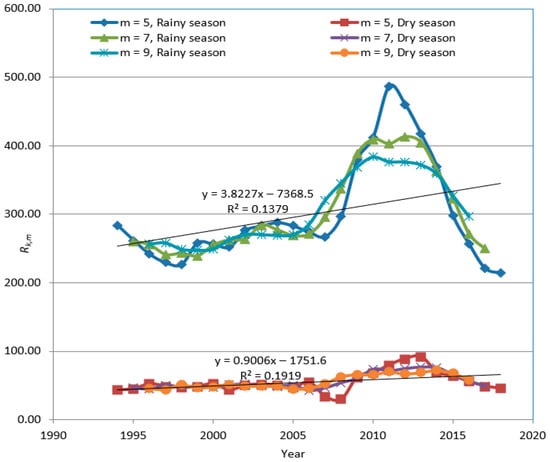
Figure 20.
Intercepts derived from the segmented regression for m = 5, m = 7, and m = 9 for rainfall in Eket. The upper data series represents the rainy season data; the lower group represents the dry season data.
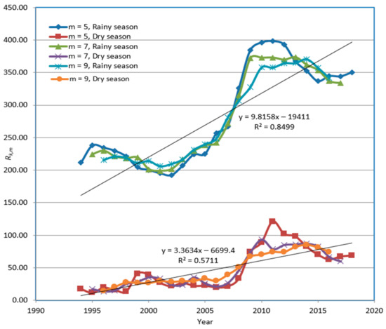
Figure 21.
Intercepts derived from the segmented regression for m = 5, m = 7, and m = 9 for rainfall in Ogoja. The upper data series represents the rainy season data; the lower group represents the dry season data.

Figure 22.
Intercepts derived from the segmented regression for m = 5, m = 7, and m = 9 for runoff in Eket. The upper data series represents the rainy season data; the lower group represents the dry season data.
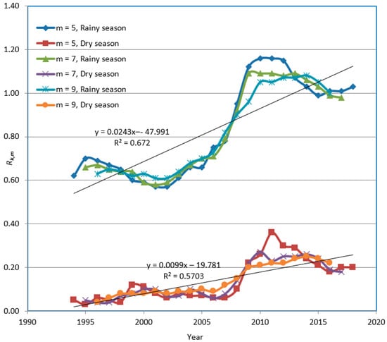
Figure 23.
Intercepts derived from the segmented regression for m = 5, m = 7, and m = 9 for runoff in Ogoja. The upper data series represents the rainy season data; the lower group represents the dry season data.
Using the annual average monthly data for the SOI and rainfall depth, the intercepts derived from the segmented regression in Eket and Ogoja show significant positive trends in both cases (Figure 20 and Figure 21). The trend in intercepts suggests there are external factors influencing rainfall other than ENSO events. Similarly, there are positive trends in the intercepts obtained from the segmented regression between the SOI and runoff at Eket and Ogoja (Figure 22 and Figure 23). The existence of a trend in the set of intercepts in all cases suggests that there are external factors influencing rainfall and runoff other than the ENSO. Furthermore, there are indications of a relationship between rainfall and runoff. Although the magnitude of the dynamic slopes for the segmented regression lines for rainfall are considerably higher than those for runoff, there is a strong correlation between the two climatic variables in most instances (Figure 16, Figure 17, Figure 18 and Figure 19). Runoff is directly proportional to rainfall, which signifies a causative relationship between them (Figure 24). A change in rainfall pattern, whether positive or negative, is expected to have a direct and similar effect on runoff, even though the impact is diminished in magnitude.
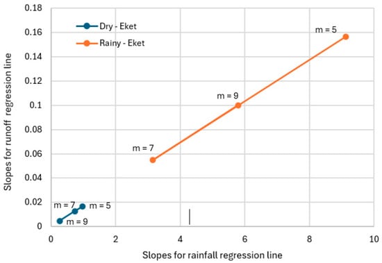
Figure 24.
Relationship between rainfall and runoff based on slopes of their segmented regression lines for m = 5, 7, and 9.
The primary objective of the ENSO analysis was to check for indications that suggest that the trend in climatic variables in the Cross River Basin was influenced by episodes of ENSO activities during the same period. The coefficient of correlation between the ENSO index (SOI) and rainfall in the Cross River Basin based on the records from Eket and Ogoja is between −0.005 in July in Eket and 0.321 in October in Ogoja. The range of values generally indicates a weak association between ENSO events and precipitation in the Cross River Basin. The coefficient of correlation between the ENSO index (SOI) and runoff in the Cross River Basin based on the records from Eket and Ogoja is between −0.004 in July in Eket and 0.321 in October. This also implies a weak association between ENSO events and runoff in the Cross River Basin. Further investigation is therefore necessary to confirm any potential effect of the ENSO on the regional climatic conditions.
The dynamic slope of the segmented regression was also used to ascertain the intensity of the impact of the ENSO events on climatic variables. The slopes were either positive or negative, implying a positive or negative impact, respectively, of ENSO events on climatic variables. The dynamic slopes of the segmented regression between the two climatic variables (i.e., annual average monthly rainfall and runoff) and SOI were calculated. Positive slope values show that the ENSO event causes a decrease in the intensity of climatic variables, while a contrasting effect occurs when the slope is negative. The magnitude of the slope is directly proportional to the rate of change, which means that the rate of change increases with the magnitude of the slope, with a reverse effect happening when the slope decreases.
Regarding rainfall, the absolute magnitude of the dynamic slopes during the rainy season (April to October) is significantly greater than those observed during the dry season (November to March), irrespective of the number of years (m-value) considered in the analysis. The maximum absolute magnitude of the dynamic slopes during the rainy season was −694.34 in 2003, whereas the maximum absolute magnitude of the dynamic slopes during the dry season was 84.58 in 2000. This illustrates the potential for ENSO events to have the most influence on rainfall during the rainy season. It is not clear how much of this observation can be attributed to the higher intensity of rainfall that is naturally prevalent during wet seasons in comparison to other periods in the year. This is contrary to what is reported by Emmanuel [52], where the absolute values of the dynamic slopes were found to be higher during the dry season in Western Africa between 1979 and 2018. signifying that the impact of the ENSO was stronger during the dry season. However, Cross River Basin was not included in the study by Emmanuel [52]. Additional analyses involving more extensive data from a much longer timescale may be required for further insights. In terms of runoff, a similar pattern is noted. The absolute magnitude of the dynamic slopes during the rainy season is greater than those observed during the dry season. The magnitude of slopes, in this case, is much lower than those obtained for rainfall, denoting that the ENSO has a smaller influence on runoff. The maximum absolute magnitude of the dynamic slopes during the rainy season was 12.18 in 2003, while the maximum absolute magnitude of the dynamic slopes during the dry season was 1.45 in 2000.
Analyses involving the dynamic slope of the segmented regression indicate the existence of an effect on rainfall and runoff by the ENSO. Nonetheless, there is a weak correlation between both climatic variables and ENSO events, which alludes to the notion that there may be other influencing factors. To confirm this, it is expedient to calculate the intercepts of the regression lines using annual average monthly SOIs and climatic variables. This is necessary to investigate the likelihood of the impact of other factors, exclusive of the ENSO events. This can be achieved by additional statistical analysis to determine the intercepts of the regression lines using annual average monthly SOIs and climatic variables. The series of intercepts calculated from the segmented regression for rainfall and runoff follows a positive trend, implying the existence of other prevailing determinants that contribute to the evolving patterns of both climatic variables. It is worthwhile to note that the set of ENSO analyses is limited to the trends in rainfall and runoff across the study period, thus excluding other climatic variables. Supplementary analyses involving other climatic indicators will be beneficial while paving the way for further validations that support the generalization of the current findings.
5. Conclusions
The trends in annual hydro-meteorological variables were studied at the regional scale for the Cross River Basin, Nigeria. In examining the time series of 11 variables for 30 years, the non-parametric Mann–Kendall test was used to analyze trends displayed by each of the variables. The study reveals that the trend in annual rainfall in Ogoja is statistically significant and positive (increasing). This is consistent with the findings of Osugiri et al. [39] based on their analysis of the trends in climatic variables in Southeast Nigeria, where the trend in rainfall intensity over the period was significant at p = 0.01. Likewise, a similar study conducted by Salami et al. [40] in the Kainji Lake Basin revealed an upward trend in rainfall, evaporation, and maximum temperature. Calabar exhibits a statistically significant and negative (decreasing) trend in rainfall, while the trends in Uyo and Eket are statistically insignificant.
The evaporation levels in Eket show a decreasing trend while those in Uyo, Calabar, and Ogoja exhibit insignificant trends. The minimum and maximum temperatures exhibit a significant upward trend at all the stations except at Ogoja station, where the temperatures exhibit a significant downward trend. The increase in temperature in the basin is in line with the global observations of a rise in temperature due to changes in climate and is consistent with the findings of Osugiri et al. [39], whose work shows an increasing trend in temperature that is statistically significant at p = 0.01. There is no significant trend in cloud cover in the basin. The relative humidity reveals a significant and increasing trend at Eket station, while there is no significant trend at Ogoja, Calabar, and Uyo stations. There is no significant trend in the soil temperature of the entire basin. The atmospheric pressure shows an upward trend in Eket only, while there is no significant trend in Uyo, Calabar, and Ogoja.
The sunshine hours indicate a downward trend in Calabar, whereas there is no significant trend in the rest of the catchment. Solar radiation shows a significant upward trend in Calabar, while in Eket, Uyo, and Ogoja, there is no significant trend. The wind speed exhibits a significant upward trend in Eket and Uyo, while in Calabar, there is a significant downward trend. This agrees with the study carried out by Ewona and Udo [54] which concluded that the trends in wind velocity and evaporation slightly decreased in Calabar due to an increase in population, which has played an important role. Calabar has experienced tremendous growth because of the renewed emphasis on tourism, urbanization, and business typified by the establishment of the TINAPA business resort. There is no significant trend in Ogoja. The behavior of the parameters might be due to variability in the climatic variables over the period considered.
This study confirms that the climatic variables that exhibit a significant upward trend have a tendency to increase with time, and their increment will be impactful, while the increment for those that are insignificant will not be impactful. Likewise, the variables that exhibit significant downward trends tend to decrease, and their reduction will be impactful, while the reduction in those that are insignificant will not be impactful. This paper provides an engineering basis for the variation in climatic parameters such as rainfall, temperature, evaporation, cloud cover, relative humidity, soil temperature, atmospheric pressure, sunshine hours, solar radiation, and wind speed in the study basin. Particularly, this study has revealed a significant downward trend in rainfall in Calabar. This is consistent with previous studies by Zitta and Madaki [41] where the rainfall anomaly index (RAI), analysis of variance, and a 5-year moving average were used to analyze 30 years of annual rainfall in Jos. The results revealed that Jos has a unimodal pattern of rainfall with a downward trend. The rainfall variability, above or below the mean value (1326.3 mm), has never exceeded 400 mm.
The findings of this study are also in accordance with Tarek et al. [42] and Ozi-Isah et al. [43], where a significant decrease in rainfall in the Sharjah UAE and Kogi States, Nigeria have been reported, respectively. Ozi-Isah et al. [43] examined the variability in rainfall, temperature, and runoff in the Niger-Benue confluence catchment in Lokoja, Kogi State, Northcentral Nigeria. Their results revealed an average decrease in rainfall of about 462.7 mm but a rise in temperature of about 3.9 °C. These had a combined effect of decreasing runoff by an average of 31.7 m3/s. The temperature increased the rate of evaporation, which helped in reducing the volume of water in the river. The multiple correlation analysis conducted by Ozi-Isah et al. [43] shows that rainfall and temperature are significantly associated with runoff. The coefficient of multiple determinations (R2) indicated that 21.6% of the changes in runoff were caused by a combination of rainfall and temperature.
The decrease in rainfall in Calabar is crucial and exacerbated by deforestation in Calabar and its surroundings and air pollution caused by heavy industrialization of the city due to the establishment of new factories, including the cement manufacturing plant, resulting in a warmer climate. The atmospheric conditions of the region do not favor cloud formation; hence, there is no significant trend in cloud cover in the basin, resulting in a decrease in rainfall. Widespread deforestation in parts of Africa and Asia is causing a decline in rainfall, leading to drought conditions [55]. All these could have serious ramifications that can impact the basin-scale management of water.
Contrarily, the reduction in evaporation and increase in rainfall in the upper belt of the Cross River Basin towards Ikom and Ogoja largely contributed to the flooding in 2022 that submerged the Ikom–Calabar highway for a period of one week. However, the reduction in rainfall, increase in evaporation, increase in solar radiation, and decrease in wind speed in Calabar will lead to a reduction in runoff in the Calabar metropolis and its surroundings. This decrease in rainfall will also have an impact on water resources (especially the reservoirs of the Kwa Falls Dam, Yakurr Dam, etc.), groundwater recharge, and other resources in the watershed.
The inconsistencies in the magnitude of climatic variables, particularly the high values recorded in some years, can be attributed to the interrelationships between climatic variables, influences of El Niño Southern Oscillation (ENSO) events, and the cumulative impact of climate change. Further studies are recommended to ascertain the nature of the interplay between climatic variables.
The findings of this study suggest that it is necessary to reevaluate the process of deriving the design rainfall for hydraulic structures in Calabar and call for the formulation of an integrated framework for water resource planning and risk assessment, considering the impact of different climate change scenarios in the basin.
Author Contributions
Conceptualization, N.M.A., J.C.A. and K.I.-I.I.E.; Methodology, N.M.A., J.C.A. and K.I.-I.I.E.; Software, N.M.A., J.C.A. and K.I.-I.I.E.; Validation, N.M.A. and K.I.-I.I.E.; Formal analysis, N.M.A., J.C.A. and K.I.-I.I.E.; Investigation, N.M.A. and K.I.-I.I.E.; Resources, N.M.A., J.C.A. and K.I.-I.I.E.; Data curation, N.M.A.; Writing—original draft, N.M.A.; Writing—review and editing, J.C.A. and K.I.-I.I.E.; Visualization, K.I.-I.I.E.; Supervision, J.C.A. and K.I.-I.I.E.; Project administration, J.C.A.; Funding acquisition, N.M.A. All authors have read and agreed to the published version of the manuscript.
Funding
This research received no external funding.
Data Availability Statement
The datasets for the period analyzed in this study are not available to the public in their entirety unless requested. However, these can be supplied by the corresponding author where requests are appropriate.
Conflicts of Interest
The authors declare no conflicts of interest.
References
- Mahmood, F.; Mohammad, H.; Golmohammadi, H.; Safavi, R.; Rasoul, M.; Hassan, A. Trend Analysis of Hydrological and Water Quality Variables to Detect Anthropogenic Effects and Climate Variability on a River Basin Scale: A Case Study of Iran. J. Hydro-Environ. Res. 2021, 34, 11–23. [Google Scholar]
- Salami, A.W.; Mohammed, A.A.; Abdulmalik, Z.H.; Olanlokun, O.K. Trend Analysis of Hydro-Meteorological Variables Using the Mann-Kendall Trend Test: Application to the Niger River and the Benue Sub-Basins in Nigeria. Int. J. Technol. 2014, 5, 100–110. [Google Scholar] [CrossRef]
- Sujeet, D.; Singh, D.K.; Islam, A.; Sarangi, A.; Khanna, M. Trend Analysis of Climatic Variables in Betwa River Basin Indian. J. Agric. Sci. 2019, 89, 1033–1038. [Google Scholar]
- Hamed, K.H.; Rao, A.R. A Modified Mann-Kendall Trend Test for Auto-Correlated Data. J. Hydrol. 1998, 204, 182–196. [Google Scholar] [CrossRef]
- Mann, H.B. Nonparametric Tests against Trend. Econometrica 1945, 13, 245–259. [Google Scholar] [CrossRef]
- Kendall, M. Rank Correlation Methods, 4th ed.; Charles Griffin: San Francisco, CA, USA, 1975. [Google Scholar]
- Rai, R.K.; Upadhyay, A.; Ojha, C.S.P. Temporal Variability of Climatic Parameters of Yamuna River Basin: Spatial Analysis of Persistence, Trend and Periodicity. Open Hydrol. J. 2010, 4, 184–210. [Google Scholar] [CrossRef]
- Barsugli, J.; Anderson, C.; Smith, J.B.; Vogel, J.M. Options for Improving Climate Modeling to Assist Water Utility Planning for Climate Change; Water Utility Climate Alliance: Washington, DC, USA, 2009; Volume 144. [Google Scholar]
- Cannarozzo, M.; Noto, L.V.; Viola, F. Spatial Distribution of Rainfall Trends in Sicily (1921–2000). Phys. Chem. Earth 2006, 31, 1201–1211. [Google Scholar] [CrossRef]
- Oguntunde, P.G.; Abiodun, B.J.; Lischeid, G. Rainfall Trends in Nigeria, 1901–2000. J. Hydrol. 2011, 411, 207–218. [Google Scholar] [CrossRef]
- Gocic, M.; Trajkovic, S. Analysis of Changes in Meteorological Variables Using Mann-Kendall and Sen’s Slope Estimator Statistical Tests in Serbia. Glob. Planet. Chang. 2013, 100, 172–182. [Google Scholar] [CrossRef]
- Gemmer, M.; Becker, S.; Jiang, T. Observed Monthly Precipitation Trends in China 1951–2002. Theor. Appl. Climatol. 2004, 77, 39–45. [Google Scholar] [CrossRef]
- Partal, T.; Kahya, E. Trend Analysis in Turkish Precipitation Data. Hydrol. Process. 2006, 20, 2011–2026. [Google Scholar] [CrossRef]
- Liu, Q.; Yang, Z.; Cui, B. Spatial and Temporal Variability of Annual Precipitation during 1961–2006 in Yellow River Basin, China. J. Hydrol. 2008, 361, 330–338. [Google Scholar] [CrossRef]
- Tabari, H. Temporal Trends and Spatial Characteristics of Drought and Rainfall in Arid and Semiarid Regions of Iran. Hydrol. Process 2012, 26, 3351–3361. [Google Scholar] [CrossRef]
- Maidment, R.I.; Allan, R.P.; Black, E. Recent Observed and Simulated Changes in Precipitation over Africa. Geophys. Res. Lett. 2015, 42, 8155–8164. [Google Scholar] [CrossRef]
- Fauchereau, N.; Trzaska, S.; Rouault, M.; Richard, Y. Rainfall Variability and Changes in Southern Africa during the 20th Century in the Global Warming Context. Nat. Hazards 2003, 29, 139–154. [Google Scholar] [CrossRef]
- Le Barbé, L.; Lebel, T.; Tapsoba, D. Rainfall Variability in West Africa during the Years 1950–90. J. Clim. 2002, 15, 187–202. [Google Scholar] [CrossRef]
- Ogungbenro, S.B.; Morakinyo, T.E. Rainfall Distribution and Change Detection across Climatic Zones in Nigeria. Weather Clim. Extrem. 2014, 5, 1–6. [Google Scholar] [CrossRef]
- Tarhule, A.; Woo, M.-K. Changes in Rainfall Characteristics in Northern Nigeria. Int. J. Climatol. 1988, 18, 1261–1271. [Google Scholar] [CrossRef]
- Akinsanola, A.; Ogunjobi, K. Analysis of Rainfall and Temperature Variability over Nigeria. Glob. J. Hum. Soc. Sci. B 2014, 14, 1–18. [Google Scholar]
- Gleick, P.H. Climate Change, Hydrology and Water Resources. Rev. Geophys. 1989, 27, 329–344. [Google Scholar] [CrossRef]
- Karpouzos, D.K.; Kavalieratou, S.; Babajimopoulos, C. Trend Analysed of Precipitation Data in Pieria Region (Greece). Eur. Water 2010, 30, 31–40. [Google Scholar]
- Mondal, A.; Kundu, S.; Mukhopadhyay, A. Rainfall Trend Analysis by Mann-Kendall Test: A Case Study of North-Eastern Part of Cuttack District, Orissa. Int. J. Geol. Earth Environ. Sci. 2012, 2, 70–78. [Google Scholar]
- Jain, S.K.; Kumar, V. Trend Analysis of Rainfall and Temperature Data for India. Curr. Sci. 2012, 102, 37–49. [Google Scholar]
- Akpabio, E.M.; Watson, N.M.; Ite, U.E.; Ukpong, I.E. Integrated Water Resources Management in the Cross River Basin, Nigeria. Int. J. Water Resour. Dev. 2007, 23, 691–708. [Google Scholar] [CrossRef]
- Akpabio, E.M. Assessing Integrated Water Resources Management in Nigeria: Insights and Lessons from Irrigation Projects in the Cross River Basin. Water Policy 2007, 9, 149–168. [Google Scholar] [CrossRef]
- Okoji, M.A. Agriculture. In Southeastern Nigeria: Its Environment; Inyang, I.B., Ed.; Abaam Press: Kaduna, Nigeria, 2001; pp. 122–134. [Google Scholar]
- NCEI. El Niño/Southern Oscillation (ENSO). Available online: https://www.ncei.noaa.gov/access/monitoring/enso/soi (accessed on 7 May 2024).
- Fersi, W.; Lézine, A.M.; Bassinot, F. Hydro-Climate Changes over Southwestern Arabia and the Horn of Africa during the Last Glacial–Interglacial Transition: A Pollen Record from the Gulf of Aden. Rev. Palaeobot. Palynol. 2016, 233, 176–185. [Google Scholar] [CrossRef]
- Gedefaw, M.; Yan, D.; Wang, H.; Qin, T.; Girma, A.; Abiyu, A.; Batsuren, D. Innovative Trend Analysis of Annual and Seasonal Rainfall Variability in Amhara Regional State, Ethiopia. Atmosphere 2018, 9, 326. [Google Scholar] [CrossRef]
- Wang, H.; Zhang, M.; Zhua, H.; Dang, X.; Yang, Z.; Yin, L. Hydro-Climatic Trends in the Last 50 Years in the Lower Reach of the Shiyang River Basin, NW China. Catena 2012, 95, 33–41. [Google Scholar] [CrossRef]
- Kahya, E.; Kalaycı, S. Trend Analysis of Streamflow in Turkey. J. Hydrol. 2004, 289, 128–144. [Google Scholar] [CrossRef]
- Degefu, M.A.; Bewket, W. Variability and Trends in Rainfall Amount and Extreme Event Indices in the Omo-Ghibe River Basin, Ethiopia. Reg. Environ. Chang. 2014, 14, 799–810. [Google Scholar] [CrossRef]
- Wang, H.; Chen, L.; Yu, X. Distinguishing Human and Climate Influences on Streamflow Changes in Luan River Basin in China. Catena 2016, 136, 182–188. [Google Scholar] [CrossRef]
- Asfaw, A.; Simane, B.; Hassen, A.; Bantider, A. Variability and Time Series Trend Analysis of Rainfall and Temperature in Northcentral Ethiopia: A Case Study in Woleka Sub-Basin. Weather Clim. Extrem. 2018, 19, 29–41. [Google Scholar] [CrossRef]
- Khambhammettu, P. Mann-Kendall Analysis. Annual Groundwater Monitoring Report; HydroGeoLogic, Inc.: Fort Ord, CA, USA, 2005. [Google Scholar]
- Ogunrinde, A.T.; Oguntunde, P.G.; Akinwumiju, A.S.; Fasinmirin, J.T. Analysis of Recent Changes in Rainfall and Drought Indices in Nigeria, 1981-2015. Hydrol. Sci. J. 2019, 64, 1755–1768. [Google Scholar] [CrossRef]
- Osugiri, I.I.; Ben-Chendo, G.N.; Okwara, M.O.; Anyanwu, G.U.; Utazi, C.O. Analysis of the Trends of Climatic Variables in Southeast Nigeria. Int. J. Curr. Res. 2019, 11, 3910–3913. [Google Scholar]
- Salami, A.; Mohammed, A.; Adeyemo, J.; Olanloku, O. Assessment of Impact of Climate Change on Runoff in the Kainji Lake Basin Using Statistical Methods. Int. J. Water Resour. Environ. Eng. 2015, 7, 7–16. [Google Scholar]
- Zitta, W.S.; Madaki, D.H. Climate Change, Rainfall Trends and Variability in Jos Plateau. J. Appl. Sci. 2020, 20, 76–82. [Google Scholar]
- Tarek, M.; Mohsin, S.; Abdallah, S. Assessment of Seasonal and Annual Rainfall Trends and Variability in Sharjah City, UAE. Adv. Meteorol. 2016, 2016, 6206238. [Google Scholar]
- Ozi-Isah, M.; Mashi, A.; Oguche, J. Examining the Variability of Rainfall, Temperature and Runoff Data in the Niger and Benue Confluence Catchment in Lokoja, Kogi State North Central, Nigeria. Int. J. Res. Hum. Resour. Manag. 2021, 3, 28–39. [Google Scholar]
- Oguntunde, P.G.; Abiodun, B.J.; Olukunle, O.J.; Olufayo, A.A. Trends and Variability in Pan Evaporation and Other Climatic Variables at Ibadan, Nigeria. Meteorol. Appl. 2012, 19, 464–472. [Google Scholar] [CrossRef]
- Solomon, O.A.; Sunday, O.U. Analysis of Trends and Variations of Monthly Mean Wind Speed Data in Nigeria. IOSR J. Appl. Phys. 2015, 7, 31–41. [Google Scholar]
- Ogolo, E. Estimation of Global Solar Radiation in Nigeria Using a Modified Angstrom Model and the Trend Analysis of the Allied Meteorological Components. Indian J. Radio Space Phys. 2014, 43, 213–224. [Google Scholar]
- Amadi, S.O.; Udo, S.O.; Pekene, D.B.; Chigbu, T.O. Study of the Trends in Sunshine Duration Hours in Nigeria during 1961-2012 Using the Linear Regression Model. Int. J. Sci. Educ. 2019, 3, 1103–1107. [Google Scholar]
- Abodunrin, T.J.; Emetere, M.E. Exploring Pressure-Temperature Trends toward Climatic Change in Ikogosi. IOP Conf. Ser. Earth Environ. Sci. 2021, 665, 012056. [Google Scholar] [CrossRef]
- Ayeni, O.D.; Oloukoi, G. Analysis of Temperature Trend as an Indicator of Climate Change Using Land Surface Temperature (LST) and Meteorological Data in Akure, Southwest Nigeria. J. Res. For. Wildl. Environ. 2022, 14, 84–100. [Google Scholar]
- Nozar, G.A.; Ghahreman, A.; Javad, B.B.; Abuzar, G.C. Trend Analysis of Soil Surface Temperature in Several Regions of Iran. In Proceedings of the 19th World Congress of Soil Science, Soil Solutions for a Changing World 74, Brisbane, Australia, 1–6 August 2010; International Union of Soil Sciences (IUSS): Brisbane, Australia, 2010. [Google Scholar]
- Osang, J.E.; Egor, A.O.; Uquetan, U.I.; Eze, B.E.; Emeruwa, C.; Pekene, D.B.J. Investigation of the Relative Humidity Profile Variations in Calabar, Nigeria. Int. J. Sci. Eng. Res. 2016, 7, 1134–1144. [Google Scholar]
- Emmanuel, I. Linkages between El Niño-Southern Oscillation (ENSO) and Precipitation in West Africa Regions. Arab. J. Geosci. 2022, 15, 671. [Google Scholar] [CrossRef]
- Susilo, G.E.; Yamamoto, K.; Imai, T.; Ishii, Y.; Fukami, H.; Sekine, M. The Effect of ENSO on Rainfall Characteristics in the Tropical Peatland Areas of Central Kalimantan, Indonesia. Hydrol. Sci. J. 2013, 58, 539–548. [Google Scholar] [CrossRef]
- Ewona, I.O.; Udo, S.O. Climatic Condition of Calabar as Typified by Some Meteorological Parameters. Glob. J. Pure Appl. Sci. 2011, 17, 81–86. [Google Scholar]
- Smith, C.; Baker, J.C.A.; Spracklen, D.V. Tropical Deforestation Causes Large Reductions in Observed Precipitation. Nature 2023, 615, 270–275. [Google Scholar] [CrossRef]
Disclaimer/Publisher’s Note: The statements, opinions and data contained in all publications are solely those of the individual author(s) and contributor(s) and not of MDPI and/or the editor(s). MDPI and/or the editor(s) disclaim responsibility for any injury to people or property resulting from any ideas, methods, instructions or products referred to in the content. |
© 2024 by the authors. Licensee MDPI, Basel, Switzerland. This article is an open access article distributed under the terms and conditions of the Creative Commons Attribution (CC BY) license (https://creativecommons.org/licenses/by/4.0/).