Abstract
This study utilizes domain adaptation to enhance the integration of diverse geoscience datasets, aiming to improve the identification of ore bodies. Traditional mineral exploration methods often face challenges in merging different geoscience data types, which leads to models that do not perform well across varying domains. Domain adaptation is a deep learning strategy aimed at adapting a model developed in one domain (source) to perform well in a different domain (target). To adapt models trained on detailed, labeled drilling data (source) to interpret broader, unlabeled geophysical data (target), Domain-Adversarial Neural Networks (DANNs) were applied, chosen for their robust performance in scenarios where the target domain does not provide labels. This approach was indirectly validated through the minimal overlap between regions identified as candidate ore and borehole locations marked as host rocks, with qualitative validation provided by t-Distributed Stochastic Neighbor Embedding (t-SNE) visualizations showing improved data integration across domains.
1. Introduction
The exploration of mineral resources is pivotal to global economic growth and technological innovation, highlighting the essential role of mining in fulfilling modern society’s demands. As accessible surface mineral deposits dwindle, the mining industry is compelled to probe deeper and more complex geological environments [1,2]. This challenge necessitates re-evaluating mineral exploration strategies to more effectively leverage the geoscience data, including geophysical, geological, and geochemical information, as well as drilling operations.
Integrating varied geoscience datasets presents significant challenges due to domain-specific differences. These differences include measurement scales, data acquisition methods, and the physical properties assessed by each technique [3]. For instance, drilling data provide precise, localized details about mineral composition at specific depths, while geophysical survey data offer a broader, albeit indirect, view of subsurface geology across large areas. These differences can be categorized into distinct ‘domains’. The challenge lies in the fact that models trained on data from one domain may not perform well when applied to data from another domain due to these inherent differences. This often leads to difficulties in creating a unified geological model, as the information from different sources may seem conflicting or misaligned, complicating the accurate identification and assessment of potential ore deposits.
Building on this complexity, the exploration of mineral resources has long been a knowledge-driven process that integrates various strands of geoscience data to identify promising exploration targets. Practitioners traditionally rely on identifying anomalies across geochemical, geophysical, and geological datasets to pinpoint areas of interest, where the convergence of multiple data sources suggests the presence of valuable ore zones beyond certain predefined thresholds. This method, deeply rooted in scientific expertise, necessitates a significant degree of subjective interpretation and judgment. The ability to accurately interpret overlapping anomalies and discern their significance is paramount, yet it introduces a level of uncertainty in determining the exact locations of prospective mineral deposits.
The introduction of machine learning technologies has precipitated a paradigm shift towards data-driven methodologies in mineral exploration. Traditional machine learning algorithms, such as Random Forest (RF) and various gradient-based methods [4,5,6], have substantially enhanced the objectivity and efficiency of analytical processes by elucidating patterns within geoscience data that may not be immediately discernible to human experts [7,8,9,10]. However, their effectiveness often diminishes when applied to new, unexplored territories due to differences between the training data and the new environments. This challenge is further complicated by the models’ tendency to rely on direct correlations between data features, which may cause them to miss indicators of mineralization.
In response to the challenges posed by domain discrepancies in mineral exploration, domain adaptation strategies are emerging as a promising approach within the realm of deep learning [11]. These strategies are designed to adapt models that have been trained in one specific domain (source) to perform effectively in a distinctly different domain (target), thereby reducing the reliance on extensive labeling of new data. This adaptive approach is particularly pertinent in geosciences, where the diversity of data types—including drilling and geophysical survey data—presents substantial challenges due to variations in scale, data acquisition techniques, and the physical properties assessed by different methods. The principal aim of domain adaptation is to facilitate the seamless integration of source and target domain data, enabling the transfer of essential information that is crucial for comprehensive exploration of mineral resources. By doing so, domain adaptation significantly improves the interpretability of geophysical survey data, bringing it into closer alignment with the detailed insights derived from drilling data, despite the fundamental differences between these data types. Although domain adaptation methods have been explored in the context of mineral prospectivity modeling in [11], the application of these techniques specifically to ore deposits is still in its early stages.
In this study, I explore the application of domain adaptation techniques to address discrepancies in mineral exploration data, with a particular focus on integrating drilling and geophysical datasets. The methodology involves adapting models originally trained on high-resolution drilling data (source domain) to enhance the interpretation of less detailed geophysical data (target domain). This process is designed to refine the identification and characterization of ore deposits by effectively leveraging the distinct strengths of both types of data. Key geophysical features such as electrical resistivity, chargeability, and susceptibility, which are critical indicators in the exploration process, are utilized.
2. Data Acquisition and Preliminary Analysis
2.1. Study Area (Pocheon, Republic of Korea)
This study focuses on the Gonamsan area, located in Northeast South Korea, known for its Yeoncheon vanadiferous titanomagnetite (TM) deposits. These deposits have been extensively mined since the early 20th century. A geological map provided in Figure 1 illustrates the Gonamsan intrusion, which measures approximately 3 km from north to south and 1.5 km from east to west.
The Gonamsan intrusion is a sill-like structure that penetrated Neoproterozoic metasedimentary rocks, which include schists, gneisses, marbles, and quartzites. This intrusion can be categorized into two main sections: the eastern section, composed of diorite–monzodiorite, diorite–gabbro, and oxide gabbro–monzodiorite, and the western section, primarily consisting of quartz monzodiorite. The Fe–Ti (–V) oxide mineralization is predominantly located in the eastern section and shows diversity in morphology, size, mineral assemblages, and chemical compositions [12,13].
The stratiform Fe–Ti (–V) oxide mineralization, interlayered with diorite–monzodiorite, is mainly found in the central part of the Gonamsan intrusion. It includes magnetite and ilmenite, along with smaller quantities of olivine, tschermakite, apatite, spinel, pyroxene, and plagioclase. Lenticular mineralization is located along the western edge of the diorite–gabbro and comprises magnetite and ilmenite with minor amounts of hornblende, apatite, chlorite, and spinel. Additionally, oxide gabbro interlayered with thin monzodiorite bands forms cyclical units irregularly scattered throughout the eastern section, containing olivine and pyroxene with minor interstitial magnetite, ilmenite, and apatite. The distinct geophysical properties of the mafic rocks within the intrusion, compared to the surrounding terrain, indicate the potential for additional mineral resources [13].
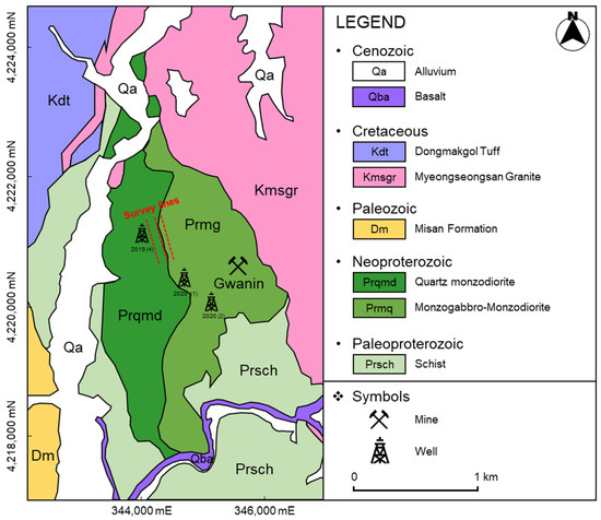
Figure 1.
Geological map of the region near the Gonamsan intrusion (reproduced from [14,15]). The well symbols mark the drilling locations, and the mine symbols indicate operational mines. The red dashed lines denote the three parallel survey lines for electrical resistivity and induced polarization.
2.2. Geophysical Survey Implementation
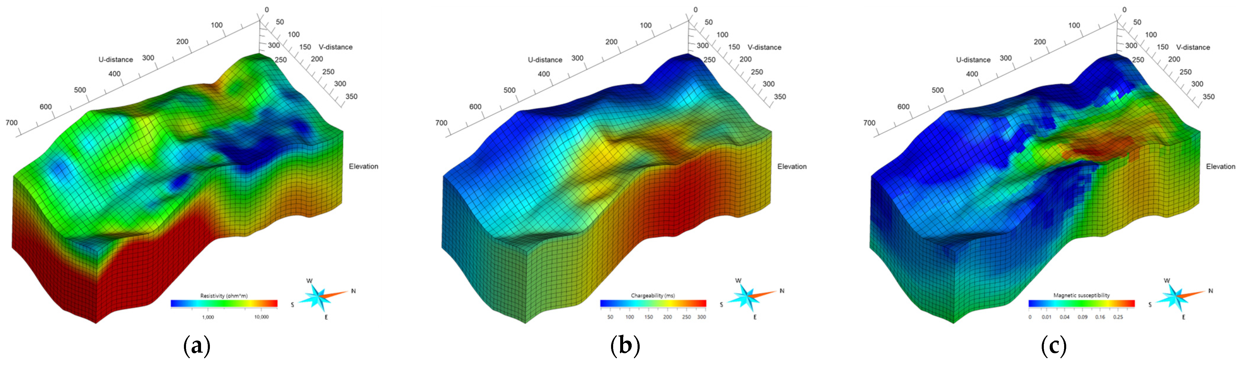
A comprehensive geophysical exploration of the Gonamsan intrusion was carried out by the Korean Institute of Geoscience and Mineral Resources (KIGAM) between 2019 and 2021 [16,17]. The exploration commenced with an airborne magnetic survey that covered the surrounding areas of the intrusion to identify magnetic anomalies indicative of potential mineral deposits. Following this preliminary survey, and based on the detected anomalies as well as considerations of terrain accessibility, more targeted surveys such as electrical resistivity and induced polarization were carried out. These surveys, illustrated along three parallel red dashed lines in Figure 1, were designed to provide detailed electrical properties of the subsurface. Data from each survey type were analyzed using inversion techniques specifically tailored for each method [16]. Figure 2 represents magnetic susceptibility, electrical resistivity, and chargeability, which were derived from airborne magnetic, electrical resistivity, and induced polarization survey data, respectively, each contributing to the identification of potential mineral zones.

Figure 2.
Three-dimensional inversion results from the geophysical field survey, displaying (a) electrical resistivity, (b) chargeability, and (c) magnetic susceptibility (reproduced from [14]).
2.3. Drilling Operations and Laboratory Experiment
In 2019 and 2020, a series of drilling projects were conducted by KIGAM in the Gonamsan intrusion, near the Gwanin magnetite mine, as depicted in Figure 1. These operations, which penetrated depths of up to 300 m, produced 541 rock samples from varied depths. The samples were classified by lithofacies—low-grade ore, gabbro, quartz monzodiorite, monzogabbro–monzodiorite, and metamorphic rocks. To prepare these for machine learning analysis, electrical resistivity, chargeability, and magnetic susceptibility were measured across all samples to maintain consistency between geophysical and drilling data [12].
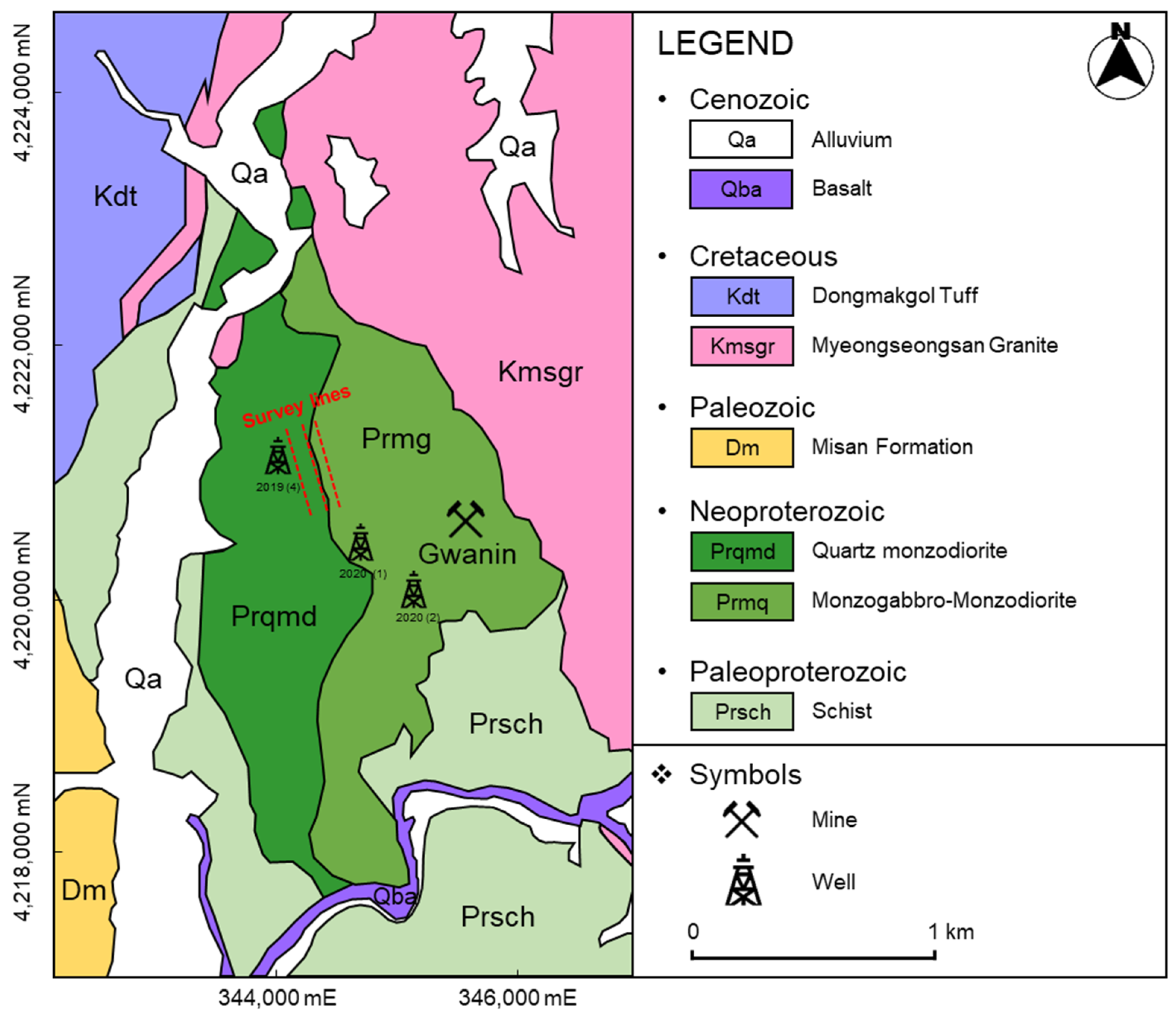
Resistivity, chargeability, and magnetic susceptibility are key geophysical properties used to explore and understand subsurface geological formations [18]. Resistivity measures the resistance a material offers to the flow of an electric current and varies with mineral content, aiding in differentiating between rock types. Low resistivity often indicates the presence of metals, important for locating ore deposits such as magnetite, which are electrically distinct from their surroundings. Chargeability measures the subsurface’s ability to retain induced electric charges, observable as the decay rate of voltage in induced polarization surveys after the cessation of current, pointing to the presence of materials like sulfide minerals. Magnetic susceptibility assesses a material’s response to an external magnetic field and is vital for detecting magnetic minerals like magnetite. Figure 3 presents the variability of these properties across different rock types via box plots. Despite their distinct ranges, the overlap in property distributions poses challenges in setting exact thresholds for ore delineation.
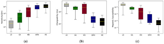
Figure 3.
Box plots displaying the distributions of (a) electrical resistivity, (b) chargeability, and (c) magnetic susceptibility for various rock types obtained from drilling data (LO: low-grade ore, GA: gabbro, MD: monzogabbro–monzodiorite, QMD: quartz monzodiorite, ME: metamorphic rocks). The median values for each rock type are marked with yellow solid lines within the box plots.
2.4. Preliminary Analysis
Data preprocessing is a necessary step in preparing geophysical properties from rock samples in drilling data for machine learning analysis. This process involves transforming raw measurements into a format suitable for predictive modeling, aiming to ensure that the processed data accurately reflect the characteristics needed to locate ore deposits within the Gonamsan intrusion.
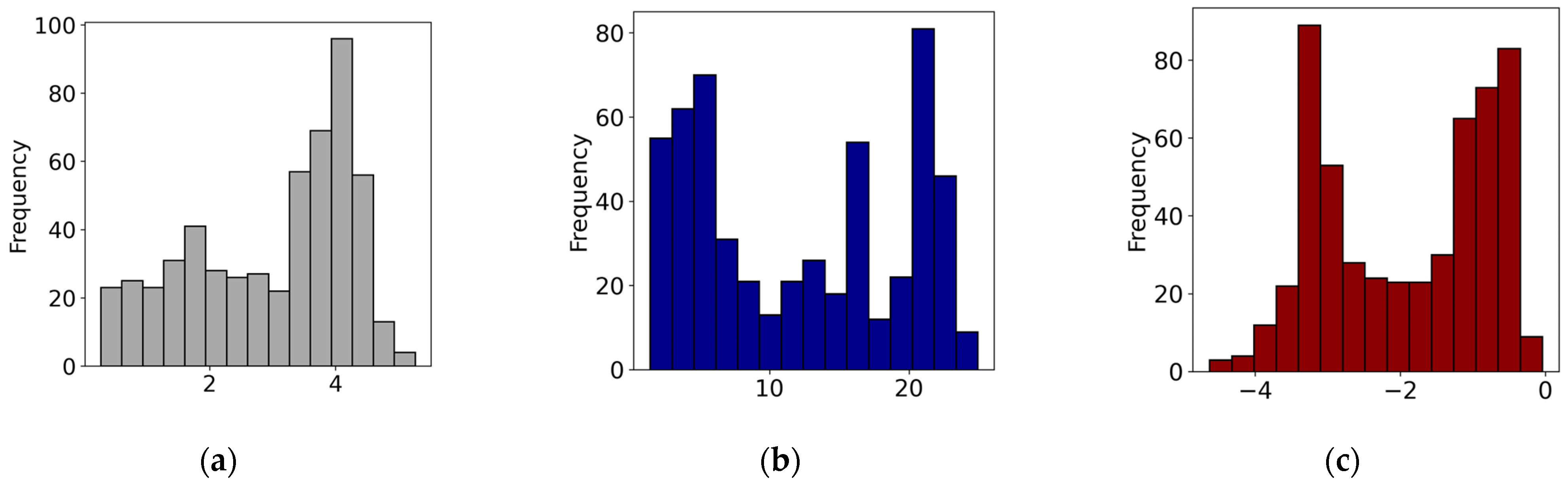
In preparation for supervised machine learning, rock samples were categorized based on their geophysical properties into ‘ORE’ and ‘HOST’ labels. A subset of these, specifically the low-grade ore samples with a density exceeding 3.6, was designated as ‘ORE’, reflecting the indication of magnetite content. The remaining 422 samples, representing a diverse range of rock types in the study area, were classified as ‘HOST’. This distinction aids in focusing the analysis on areas that may contain mineral deposits. To address the skewness in the dataset, logarithmic transformations were applied to resistivity and magnetic susceptibility, while a square root transformation was used for chargeability [19]. Figure 4 illustrates the data distributions after applying these transformations. Subsequently, the data were standardized to achieve a more normal distribution. The dataset was divided into training and testing sets with 80% of the data allocated for training and the remaining 20% for testing. Given the imbalance with a larger number of ‘HOST’ samples compared to ‘ORE’, the ADASYN (Adaptive Synthetic Sampling Approach for Imbalanced Learning) method [20,21] was employed to generate synthetic ‘ORE’ samples, enhancing dataset balance. This technique creates synthetic samples by randomly selecting among the k nearest ‘ORE’ neighbors of an ‘ORE’ sample and placing the synthetic sample on the line connecting them. This adaptive approach increases ‘ORE’ representation, particularly in areas heavily influenced by ‘HOST’ samples, thus aiding the model in better generalizing from the data. After applying ADASYN, the numbers of ‘HOST’ and ‘ORE’ samples were adjusted to 353 and 337, respectively.

Figure 4.
Data distributions after transformations: (a) log-transformed electrical resistivity, (b) square root-transformed chargeability, and (c) log-transformed magnetic susceptibility.
3. Methods
3.1. Overview of Domain Adaptation Techniques
The inherent challenge of integrating diverse geoscience datasets for mineral exploration is magnified by domain discrepancies that traditional machine learning models often cannot overcome. These discrepancies, arising from variations in measurement scales and data acquisition methods across different geological settings, hinder the models’ ability to generalize from one domain to another. Domain adaptation techniques address this challenge by adjusting models to perform effectively across these varied domains. By enabling the integration of drilling and geophysical survey data, despite their inherent differences, domain adaptation holds the potential to enhance the identification and characterization of ore deposits [11].
Domain adaptation techniques mitigate the gap between different data domains, crucial for models trained on data from one domain (source) and tested on another (target) [22]. These methods are essential for enhancing model performance when direct application from one domain to another might otherwise result in significant performance degradation. Domain adaptation involves training a model in such a way that it can generalize knowledge from one domain and apply it to another. This is achieved through several strategies, including adversarial training and feature alignment. Adversarial training involves training a model with a domain discriminator, which introduces an adversarial loss to minimize the distinguishability between domains. Feature alignment ensures that the feature distributions of the source and target domains are similar, allowing the model to generalize better. The wide range of domain adaptation strategies can be categorized into three main approaches, each addressing the challenges of domain discrepancies in a fundamental manner:
- Feature-based adaptation: This approach aligns the feature spaces of the source and target domains to minimize domain differences, ensuring that models perform consistently across both. The principle involves transforming or finding common representations of features that reduce discrepancies. Representative methods include Transfer Component Analysis (TCA) [23] and Deep Correlation Alignment (Deep CORAL) [24].
- Adversarial-based adaptation: Inspired by adversarial training, this strategy trains models to produce features that a domain classifier cannot distinguish between do-mains, promoting domain-invariant feature generation. Key techniques are Domain-Adversarial Neural Networks (DANNs) [25], Conditional Domain Adversarial Networks (CDANs) [26], and Adversarial Discriminative Domain Adaptation (ADDA) [27].
- Discrepancy-based adaptation: Focusing on directly minimizing statistical differences in feature distributions between domains, this method aims to bridge the gap by adjusting model representations. Techniques such as Maximum Classifier Discrepancy (MCD) [28] and Kernel Mean Matching (KMM) [29] are utilized to achieve this goal.
3.2. Domain Adaptation in Geophysics
The integration of diverse geoscience datasets for mineral exploration presents significant challenges due to domain discrepancies. These discrepancies arise from variations in measurement scales, data acquisition methods, and the physical properties assessed across different geological settings. The effectiveness of domain adaptation techniques in geophysics can be influenced by several factors related to the characteristics of data and domains.
One critical factor is the availability of labeled data in the target domain, which can affect the choice of adaptation strategy. The lack of such data may limit some methods [30]. Adaptation methods need to be able to handle these discrepancies, effectively utilizing source data while accommodating the larger scale of target domain data [31]. Furthermore, the degree of similarity in feature distributions across domains is crucial, as divergent feature spaces necessitate methods capable of facilitating a connection [32,33]. This need for alignment and balance, particularly in unsupervised settings, is underscored by approaches that focus on aligning both marginal and conditional feature distributions as discussed in [33]. Therefore, ensuring the selection and application of adaptation techniques that align with these varied conditions is necessary for advancing the accuracy and reliability of geophysical analyses in mineral exploration.
The geophysical dataset provides a wide-ranging, unlabeled view of subsurface geology, encompassing a broader spectrum of geological features without direct annotations. Given these considerations, the DANN appears to be particularly well suited for addressing the specific requirements of this study. This technique stands out in minimizing domain discrepancies through adversarial training, which pushes feature extractors to produce indistinguishable features across domains, a crucial attribute in scenarios where the target domain lacks labels [25]. This allows for effective alignment of feature distributions without dependence on target labels. In contrast, other methods such as CDAN, MCD, DeepCORAL, and ADDA do not perform as well under these specific conditions: CDAN and ADDA require labeled target data that I do not have [26,27], MCD demands careful tuning to avoid divergence that does not genuinely represent domain adaptation [28], and DeepCORAL, while aligning basic statistical properties, may fail to address more complex semantic differences [24].
3.3. Implementation of Domain Adaptation
The implementation of the DANN model was carried out using the Adapt library [34], which facilitates the application of domain adaptation techniques. The DANN model in this study was constructed with three main components, the encoder, the task model, and the discriminator, each customized for specific needs.
The encoder consists of two dense layers with ReLU activation functions, which transform the input features into a suitable representation. The task model, also composed of two dense layers with ReLU activation, followed by an output layer with a sigmoid activation function, is responsible for performing the primary prediction task. The discriminator model, similar in structure to the encoder and task models, is designed to distinguish between the source and target domain features. Each model is compiled with the Adam optimizer and binary cross-entropy loss. To optimized the training model, hyperparameters including lambda values, learning rates, batch sizes, and the number of epochs were considered. The lambda parameter in DANN controls the trade-off between the task-specific loss and the domain adaptation loss, effectively balancing the model’s ability to perform well on the source domain while adapting to the target domain [25].
For model evaluation, the silhouette score was employed as a metric to select the best hyperparameters for DANN. This metric, which assesses the degree of separation between clusters and ranges from −1 to 1, is particularly valuable in scenarios without labeled target data [35]. A higher silhouette score indicates that the model effectively groups data points into distinct clusters, important for evaluating the success of the domain adaptation.
4. Results
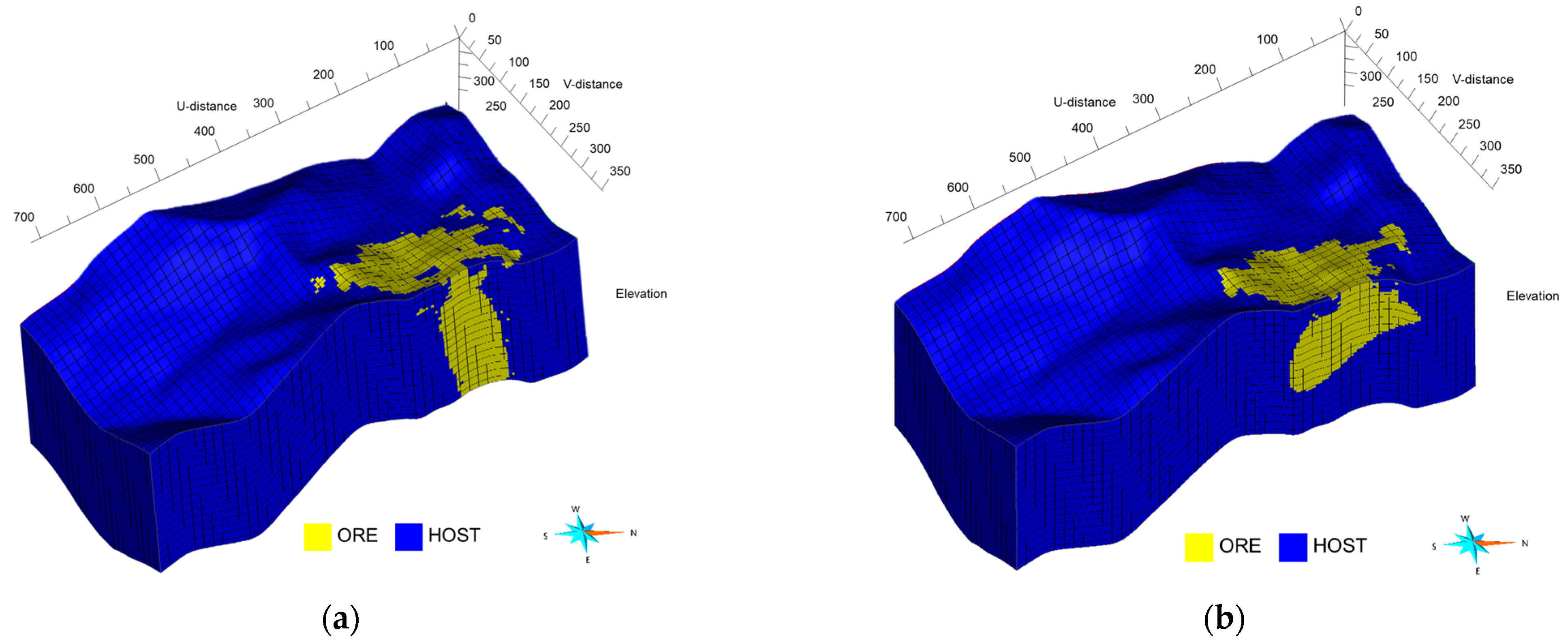
Figure 5 presents the outcomes of applying the DANN-trained model to the geophysical survey area, alongside results from an RF model trained solely on the source domain data for comparison. Both models identified ORE locations predominantly in the northeast direction, aligning with findings reported in [15].

Figure 5.
Classification outcomes in the geophysical survey region from (a) an RF model trained on source domain data and from (b) a DANN model adapted across domains.
Table 1 displays the performance metrics of both the DANN-trained model and the RF model when applied to the test data from the source domain. These metrics include accuracy, recall score, precision, and F1 score. Accuracy measures the proportion of correct predictions among the total number of cases processed. Recall score, also known as sensitivity, measures the proportion of actual positives correctly identified by the model. Precision measures the proportion of positive predictions that are actually correct. F1 score is the harmonic mean of precision and recall, providing a single metric that balances both concerns. While the performance on source domain test data does not directly validate the results on the target domain, it provides insights into the generalizability of the models.

Table 1.
Performance metrics of RF and DANN models on geophysical data.
The DANN model, trained using an adversarial approach, is designed to minimize distinguishability between source and target domain data. If it fails to accurately classify source domain test data, this raises concerns about whether it has adequately learned the source domain’s characteristics, potentially undermining its effectiveness. The results in Table 1, showing no significant difference in performance between the DANN and RF models, suggest that the DANN model maintains its effectiveness in the source domain. This indicates that the adaptation process has not compromised the model’s original predictive capabilities.
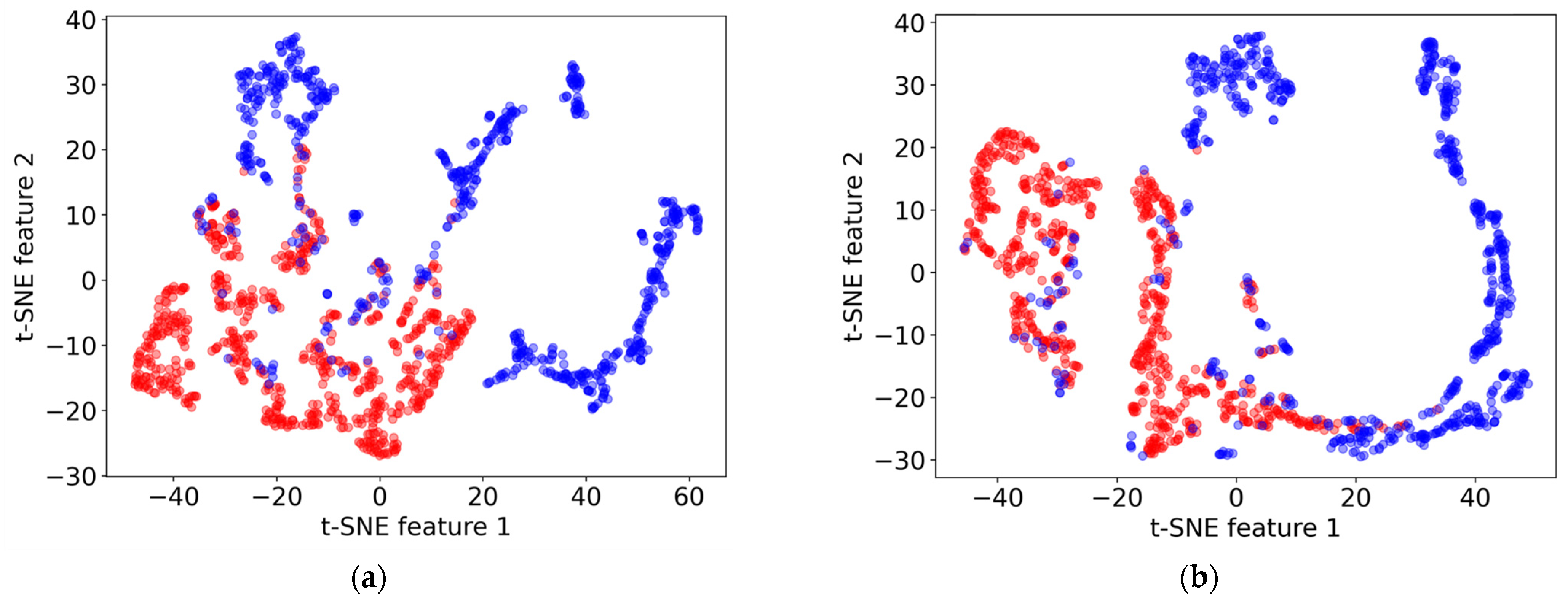
To qualitatively assess clustering, t-SNE (t-Distributed Stochastic Neighbor Embedding) [36] was employed, as visualized in Figure 6. This figure presents the clustering of source and target domain data before and after applying the DANN model, with red dots representing the source domain (borehole data) and blue dots representing the target domain (geophysical survey data). Features 1 and 2 in the t-SNE plot are the two-dimensional representations obtained through the t-SNE algorithm, used to visualize high-dimensional data in a reduced feature space. Ideally, effective domain adaptation would result in a significant overlap of the two domains in the t-SNE plot after training. However, while there is some improvement in the alignment of the domains post-adaptation, the change is not substantial. This modest enhancement suggests the inherent challenges of reconciling significant differences between drilling and geophysical data through domain adaptation.
Figure 6.
t-SNE visualizations illustrating the clustering of data points (a) before and (b) after applying the Domain-Adversarial Neural Network (DANN) model. Red dots represent the source domain (drilling data), and blue dots represent the target domain (geophysical survey data). Features 1 and 2 are the two-dimensional representations obtained through the t-SNE algorithm, used to visualize high-dimensional data in a reduced feature space.
5. Discussion
5.1. Properties of Drilling and Geophysical Data
Understanding the correlation among features in different datasets is helpful. Table 2 summarizes the means, standard deviations, and correlations of the transformed features (log-transformed resistivity, square root-transformed chargeability, and log-transformed magnetic susceptibility) for both rock samples and field data. The analysis of feature correlations reveals a general agreement in how features are related, despite some differences in the exact correlation values. This suggests that, at a basic level, the geological features captured by both datasets are similar, supporting the idea of integrating them through domain adaptation.
Table 2.
Mean, standard deviation (SD), and correlations of log-transformed resistivity (LOGRESI), square root-transformed chargeability (SQRTCHAR), and log-transformed magnetic susceptibility (LOGSI) for both rock samples and field data.
To apply the domain adaptation techniques, 690 data points were sampled from the target domain (geophysical data) to match the number of samples found in the drilling data. The three features—logarithmic magnetic susceptibility, square root chargeability, and logarithmic resistivity—were evaluated using the Kolmogorov–Smirnov (KS) test statistic and p-values. The KS test is a nonparametric test that compares the distributions of two datasets, assessing whether they differ significantly [37]. It is suitable for these evaluations because it helps to determine whether the sample distributions from the target domain effectively capture the characteristics of the drilling data. The results were (0.037, 0.288) for LOGSI, (0.033, 0.401) for SQRTCHAR, and (0.038, 0.244) for LOGRESI, respectively, indicating that the sampling effectively captures the characteristics of the target domain dataset.
5.2. Evaluation of Classification Outcomes
It is necessary to evaluate the extent to which the classification outcomes align with the borehole lithology data from the Gonamsan area. Figure 7 illustrates the areas classified as ORE based on the outcomes from both the RF and DANN-trained models, alongside borehole lithology data from the area of interest in the target domain. Unfortunately, the available borehole data from four drill cores obtained from the exploration area shown in Figure 1 only include HOST labels, limiting the ability to directly verify the model’s predictions against confirmed ORE presence. However, the absence of overlap between the regions identified as ORE and the locations of the HOST-labeled boreholes provides an indirect validation of the models’ classifications. The RF model’s ORE predictions showed more overlap with HOST-labeled borehole locations than the DANN model, suggesting that the DANN model may align better with the subsurface geological context indicated by the borehole data. The geophysical survey results support these model predictions. The results presented in Figure 2 highlight a distinct zone to the northeast of the explored region, characterized by unusually low electrical resistivity and high chargeability and magnetic susceptibility. These geophysical characteristics indicate the likely presence of mineral resources, aligning with the DANN model’s predictions.
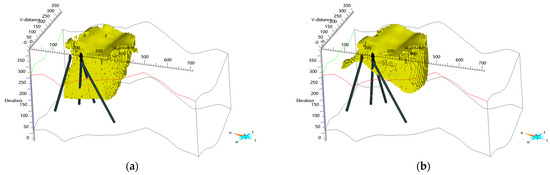
Figure 7.
Classification results marking areas as ‘ORE’ in the geophysical survey area from Figure 6: (a) the RF model and (b) the DANN-trained model, shown alongside borehole lithology data from the target domain.
The DANN model’s predictions are consistent with the known geological features of the Gonamsan area as depicted in Figure 1. Figure 8 presents a comparison between the geological map (an enlarged view of Figure 1) and the classification results obtained with the trained DANN model. The areas colored in yellow are candidates for ore deposits, as predicted by the model. Although a three-dimensional interpretation could not be verified due to the limitations in terms of available data, the eastern section, known for its Fe–Ti (–V) oxide mineralization, corresponds well in the two-dimensional plane with the areas predicted as ORE by the model.
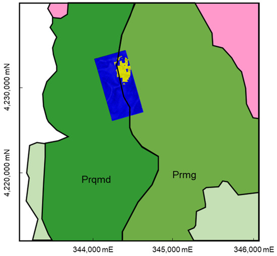
Figure 8.
Comparison between the geological map (an enlarged view of Figure 1) and classification results obtained with the trained DANN model. The areas colored in yellow are candidates for ore deposits, as predicted by the model.
5.3. Limitations in Data and Techniques
A primary limitation in this study is the absence of labeled data in the target domain, which is crucial for verifying the accuracy of predictions from supervised learning models. Without these labels, indirect methods of evaluation had to be employed, such as analyzing spatial distributions and utilizing statistical measures like the silhouette score. These methods, while insightful, cannot provide the definitive confirmation that direct empirical validation would offer. Additionally, the limited number of borehole data samples and the absence of significant ore bodies in the source domain restricted the potential for robust supervised learning. Ideally, labels in geoscience supervised learning should reflect precise ore grades. However, the absence of such specific grading information severely hindered our ability to train models effectively.
The difference in resolution between the source (borehole data) and target (geophysical survey data) domains presented a challenge. Despite using a domain adaptation technique, the variations in detail and resolution between these domains affected their effectiveness. This resolution difference highlights the challenges involved in applying models trained on high-resolution source data to lower-resolution target data while trying to maintain accuracy and detail.
The geophysical data used in this study were derived from inversion processes, which depend heavily on specific acquisition parameters and interpretation techniques. As a result, these measurements are not unique values but estimates that can vary significantly based on the methodology employed. This variability adds a layer of complexity in ensuring that domain adaptation accurately reflects geological realities, presenting challenges in working with derived rather than direct measurements.
6. Conclusions
This study demonstrated the application of domain adaptation to bridge the gap between diverse geoscience datasets, enhancing mineral exploration. Models trained on detailed, labeled drilling data were adapted to interpret broader, unlabeled geophysical data, effectively maintaining predictive capabilities across different domains. The DANN model was chosen for its ability to effectively adapt features across domains without needing labeled data from the target domain. The model was evaluated using the silhouette score, which confirmed its effectiveness in clustering data. It performed well on test data from the source domain, successfully learning and adapting to the data characteristics. Although the borehole data from the target domain included only HOST labels, it was used to indirectly validate the model’s predictive accuracy. The absence of overlap with areas classified as ORE by the trained model suggests that it identified geological features. Additionally, t-SNE visualizations showed a reduction in differences between the source and target domain feature spaces.
These results collectively underscore the utility of domain adaptation techniques in overcoming dataset discrepancies in geoscience, leading to more accurate and effective mineral exploration strategies. By integrating diverse data sources and reducing label dependence, this approach shows promise in enhancing the generalizability of models across different geological settings. The findings suggest that domain adaptation could be a useful tool in geosciences, helping to improve the consistency and accuracy of mineral exploration efforts.
Funding
This research was supported by the National Research Foundation of Korea (NRF) grant funded by the Korea government (MSIT) (No. 2023-00212423) and also was supported by the research grant of the Gyeongsang National University in 2022.
Data Availability Statement
The original contributions presented in the study are included in the article, further inquiries can be directed to the corresponding author.
Acknowledgments
I appreciate anonymous reviewers and the associated editor for the constructive comments to improve the quality of the manuscript. Gratitude is also extended to the Korean Institute of Geoscience and Mineral Resources (KIGAM) for providing the drilling and geophysical survey data used in this study.
Conflicts of Interest
The author declares no conflicts of interest.
References
- Wang, S.; Liu, H.; Li, L.; Zhang, C. Editorial: Geological disasters and its prevention in deep mining. Front. Earth Sci. 2022, 10, 1071841. [Google Scholar] [CrossRef]
- Xie, H.; Ju, Y.; Gao, F.; Gao, M.; Zhang, R. Groundbreaking theoretical and technical conceptualization of fluidized mining of deep underground solid mineral resources. Tunn. Undergr. Space Technol. 2017, 67, 68–70. [Google Scholar] [CrossRef]
- Bergen, K.; Johnson, P.; Hoop, M.; Beroza, G. Machine learning for data-driven discovery in solid Earth geoscience. Science 2019, 363, eaau0323. [Google Scholar] [CrossRef]
- Rodriguez-Galiano, V.; Sánchez-Castillo, M.; Chica-Olmo, M.; Chica-Rivas, M. Machine learning predictive models for mineral prospectivity: An evaluation of neural networks, random forest, regression trees and support vector machines. Ore Geol. Rev. 2015, 71, 804–818. [Google Scholar] [CrossRef]
- Chaudhari, A.; Khandelwal, H.; Khan, A.; Kurade, O.; Kolekar, A. Mineral Prediction Using Random Forest Classifier. In Proceedings of the 14th International Conference on Computing Communication and Networking Technologies (ICCCNT), Delhi, India, 6–8 July 2023; IEEE: Piscataway, NJ, USA, 2023; pp. 1–6. [Google Scholar] [CrossRef]
- Ford, A. Practical Implementation of Random Forest-Based Mineral Potential Mapping for Porphyry Cu–Au Mineralization in the Eastern Lachlan Orogen, NSW, Australia. Nat. Resour. Res. 2019, 29, 267–283. [Google Scholar] [CrossRef]
- Carranza, E.; Laborte, A. Data-Driven Predictive Modeling of Mineral Prospectivity Using Random Forests: A Case Study in Catanduanes Island (Philippines). Nat. Resour. Res. 2016, 25, 35–50. [Google Scholar] [CrossRef]
- Breiman, L. Random forests. Mach. Learn. 2001, 45, 5–32. [Google Scholar] [CrossRef]
- Chen, T.; Guestrin, C. XGBoost: A Scalable Tree Boosting System. In Proceedings of the 22nd ACM SIGKDD International Conference on Knowledge Discovery and Data Mining, New York, NY, USA, 13–17 August 2016; pp. 785–794. [Google Scholar] [CrossRef]
- Ke, G.; Meng, Q.; Finley, T.; Wang, T.; Chen, W.; Ma, W.; Ye, Q.; Liu, T.Y. LightGBM: A highly efficient gradient boosting decision tree. Adv. Neural Inf. Process. Syst. 2017, 30, 3146–3154. Available online: https://dl.acm.org/doi/10.5555/3294996.3295074 (accessed on 2 July 2024).
- Zheng, Y.; Deng, H.; Wu, J.; Wang, R.; Liu, Z.; Wu, L.; Mao, X.; Chen, J. Space-associated domain adaptation for three-dimensional mineral prospectivity modeling. Int. J. Digit. Earth 2023, 16, 2885–2911. [Google Scholar] [CrossRef]
- Shin, S.; Cho, S.; Kim, E.; Lee, J. Geophysical Properties of Precambrian Igneous Rocks in the Gwanin Vanadiferous Titanomagnetite Deposit, Korea. Minerals 2021, 11, 1031. [Google Scholar] [CrossRef]
- Lee, J.; Yang, S.; White, N.C.; Shin, D.; Kim, E.J. Whole-rock geochemistry and mineral compositions of gabbroic rocks and the associated Fe–Ti (–V) oxide deposit in the Gonamsan intrusion, South Korea. Ore Geol. Rev. 2022, 148, 105054. [Google Scholar] [CrossRef]
- Kee, W.S.; Cho, D.L.; Kim, B.C.; Jin, K.M. Geological Report of the Pocheon Sheet (1:50,000); Korea Institute of Geoscience and Mineral Resources: Daejeon, Republic of Korea, 2005; p. 66. [Google Scholar]
- Shin, Y.; Shin, S. Rock classification in a vanadiferous titanomagnetite deposit based on supervised machine learning. Minerals 2022, 12, 461. [Google Scholar] [CrossRef]
- Son, J.-S.; Shin, S.; Park, S.-G. Development of Three-dimensional Inversion Algorithm of Complex Resistivity Method. Geophys. Explor. 2021, 24, 180–193. [Google Scholar] [CrossRef]
- Kim, B.; Jeong, S.; Bang, E.; Shin, S.; Cho, S. Investigation of iron ore mineral distribution using aero-magnetic exploration techniques: Case study at Pocheon, Korea. Minerals 2021, 11, 665. [Google Scholar] [CrossRef]
- Telford, W.M.; Geldart, L.P.; Sheriff, R.E. Applied Geophysics; Cambridge University Press: Cambridge, UK, 1990. [Google Scholar]
- Feng, C.; Wang, H.; Lu, N.; Chen, T.; He, H.; Tu, X.M. Log-transformation and its implications for data analysis. Shanghai Arch. Psychiatry 2014, 26, 105–109. [Google Scholar]
- He, H.; Bai, Y.; Garcia, E.A.; Li, S. ADASYN: Adaptive synthetic sampling approach for imbalanced learning. In Proceedings of the 2008 IEEE International Joint Conference on Neural Networks (IEEE World Congress on Computational Intelligence), Hong Kong, China, 1–6 June 2008; pp. 1322–1328. [Google Scholar]
- Tang, B.; He, H. KernelADASYN: Kernel based adaptive synthetic data generation for imbalanced learning. In Proceedings of the 2015 IEEE Congress on Evolutionary Computation (CEC), Sendai, Japan, 25–28 May 2015; pp. 664–671. [Google Scholar] [CrossRef]
- Wang, Z.; Du, B.; Guo, Y. Domain Adaptation with Neural Embedding Matching. IEEE Trans. Neural Netw. Learn. Syst. 2020, 31, 2387–2397. [Google Scholar] [CrossRef]
- Pan, S.J.; Tsang, I.W.; Kwok, J.T.; Yang, Q. Domain adaptation via transfer component analysis. IEEE Trans. Neural Netw. 2009, 22, 199–210. [Google Scholar] [CrossRef]
- Sun, B.; Saenko, K. Deep CORAL: Correlation alignment for deep domain adaptation. In Proceedings of the European Conference on Computer Vision (ECCV) Workshops, Amsterdam, The Netherlands, 11–14 October 2016; pp. 443–450. [Google Scholar] [CrossRef]
- Ganin, Y.; Lempitsky, V. Unsupervised domain adaptation by backpropagation. In Proceedings of the 32nd International Conference on Machine Learning (ICML), Lille, France, 6–11 July 2015; pp. 1180–1189. [Google Scholar]
- Long, M.; Cao, Z.; Wang, J.; Jordan, M.I. Conditional adversarial domain adaptation. In Proceedings of the Advances in Neural Information Processing Systems (NeurIPS), Montreal, QC, Canada, 3–8 December 2018; pp. 1640–1650. [Google Scholar] [CrossRef]
- Tzeng, E.; Hoffman, J.; Saenko, K.; Darrell, T. Adversarial discriminative domain adaptation. In Proceedings of the IEEE Conference on Computer Vision and Pattern Recognition (CVPR), Honolulu, HI, USA, 21–26 July 2017; pp. 7167–7176. [Google Scholar] [CrossRef]
- Saito, K.; Watanabe, K.; Ushiku, Y.; Harada, T. Maximum classifier discrepancy for unsupervised domain adaptation. In Proceedings of the IEEE Conference on Computer Vision and Pattern Recognition (CVPR), Salt Lake City, UT, USA, 18–22 June 2018; pp. 3723–3732. [Google Scholar] [CrossRef]
- Huang, J.; Gretton, A.; Borgwardt, K.; Schölkopf, B.; Smola, A.J. Correcting sample selection bias by unlabeled data. In Proceedings of the Neural Information Processing Systems, Vancouver, BC, Canada, 4–7 December 2006. [Google Scholar]
- Pan, S.J.; Yang, Q. A survey on transfer learning. IEEE Trans. Knowl. Data Eng. 2010, 22, 1345–1359. [Google Scholar] [CrossRef]
- Glorot, X.; Bordes, A.; Bengio, Y. Domain adaptation for large-scale sentiment classification: A deep learning approach. In Proceedings of the 28th International Conference on Machine Learning (ICML-11), Bellevue, WA, USA, 28 June–2 July 2011; pp. 513–520. [Google Scholar]
- Long, M.; Cao, Y.; Wang, J.; Jordan, M.I. Learning transferable features with deep adaptation networks. In Proceedings of the International Conference on Machine Learning, Lille, France, 6–11 July 2015; pp. 97–105. [Google Scholar]
- Wang, Z.; Wang, X.; Liu, F.; Gao, P.; Ni, Y. Adaptative balanced distribution for domain adaptation with strong alignment. IEEE Access 2021, 9, 100665–100676. [Google Scholar] [CrossRef]
- Mathelin, A.; Atiq, M.; Richard, G.; de la Concha, A.; Yachouti, M.; Deheeger, F.; Vayatis, N. Adapt: Awesome domain adaptation python toolbox. arXiv 2021, arXiv:2107.03049. [Google Scholar] [CrossRef]
- Shahapure, K.R.; Nicholas, C.K. Cluster Quality Analysis Using Silhouette Score. In Proceedings of the 2020 IEEE 7th International Conference on Data Science and Advanced Analytics (DSAA), Sydney, Australia, 6–9 October 2020; pp. 1322–1328. [Google Scholar] [CrossRef]
- Van Der Maaten, L. Barnes-hut-SNE. arXiv 2013, arXiv:1301.3342. [Google Scholar] [CrossRef]
- Zheng, W.; Lai, D.; Gould, K.L. A simulation study of a class of nonparametric test statistics: A close look of empirical distribution function-based tests. Commun. Stat. Simul. Comput. 2023, 52, 1132–1148. [Google Scholar] [CrossRef]


Disclaimer/Publisher’s Note: The statements, opinions and data contained in all publications are solely those of the individual author(s) and contributor(s) and not of MDPI and/or the editor(s). MDPI and/or the editor(s) disclaim responsibility for any injury to people or property resulting from any ideas, methods, instructions or products referred to in the content. |
© 2024 by the author. Licensee MDPI, Basel, Switzerland. This article is an open access article distributed under the terms and conditions of the Creative Commons Attribution (CC BY) license (https://creativecommons.org/licenses/by/4.0/).