The Preparation Phase of the 2022 M_L 5.7 Offshore Fano (Italy) Earthquake: A Multiparametric–Multilayer Approach

Abstract

This paper presents an analysis of anomalies detected during the preparatory phase of the 9 November 2022 M_L = 5.7 earthquake, occurring approximately 30 km off the coast of the Marche region in the Adriatic Sea (Italy). It was the largest earthquake in Italy in the last 5 years. According to lithosphere–atmosphere–ionosphere coupling (LAIC) models, such earthquake could induce anomalies in various observable variables, from the Earth’s surface to the ionosphere. Therefore, a multiparametric and multilayer approach based on ground and satellite data collected in each geolayer was adopted. This included the revised accelerated moment release method, the identification of anomalies in atmospheric parameters, such as Skin Temperature and Outgoing Longwave Radiation, and ionospheric signals, such as Es and F2 layer parameters from ionosonde measurements, magnetic field from Swarm satellites, and energetic electron precipitations from NOAA satellites. Several anomalies were detected in the days preceding the earthquake, revealing that their cumulative occurrence follows an exponential trend from the ground, progressing towards the upper atmosphere and the ionosphere. This progression of anomalies through different geolayers cannot simply be attributed to chance and is likely associated with the preparation phase of this earthquake, supporting the LAIC approach.

1. Introduction

The study of a possible coupling mechanism between the lithosphere, atmosphere, and ionosphere, also known as lithosphere–atmosphere–ionosphere coupling (LAIC), before an earthquake (EQ) or a volcanic eruption, is becoming increasingly relevant within the scientific community. Prior to the occurrence of such geophysical events, the Earth emits transient signals, sometimes strong but more often subtle and fleeting, which can manifest as local variations in the magnetic field, electromagnetic emissions across a wide range of frequencies (mostly 0.001 Hz–100 KHz, i.e., ULF-ELF-VLF), and a variety of atmospheric and ionospheric phenomena. This is a rather complex mechanism and there is considerable uncertainty about the nature of the processes that could produce these signals, both within the Earth’s crust and on its surface. Over the years, various models have been developed to suggest a connection, i.e., coupling, among the geolayers following different channels.

Hayakawa [1] proposed three channels to establish connections between different observations in each layer: the chemical channel (also known as the electric field channel), the acoustic gravity wave (AGW) channel, and the electromagnetic (EM) channel. Freund [2] proposed an electrostatic channel in which stressed rocks release positive charge carriers known as “positive holes”. Dahlgren et al. [3] contested this theory, in particular studies [4,5,6]. Scoville et al. [7] pointed out some pitfalls in the experiment.

Pulinets and Ouzounov [8] proposed a radon release from the crust in the earthquake preparation zone; radon is the radioactive gas produced in the decay chain of uranium or thorium emitted from the ground, affecting the electric field in the troposphere–ionosphere electric circuit. Surkov et al. [9] further investigated the potential impact of radon emissions on the atmosphere and ionosphere, finding that localized changes in atmospheric currents due to radon have minimal effects on the electron distribution in the ionosphere. Similarly, the study proposed by Schekotov et al. [10] does not find clear connections between electromagnetic variations and changes in pre-seismic temperatures, casting doubt on the hypothesis that radon emissions influence the ionosphere.

To explain seismo-ionospheric effects, other authors [11,12,13] suggested atmospheric processes producing acoustic and/or gravity waves in the seismic preparation region. Investigating LAIC processes, the multiparametric analysis around earthquakes has become a highly debated topic, involving various parameters across layers and utilizing different observation technologies within the same layer. A comprehensive study [14] on investigating the LAIC mechanism of the Mw = 7.2 Haiti earthquake on 14 August 2021, considered 52 precursors, including GPS Total Electron Content (TEC), 4 from CSES-01 satellite data, 7 lithospheric and atmospheric precursors from AIRS and OMI sensors, and 40 from the Swarm satellite constellation. This author observed a significant amount of anomalous values, suggesting a sequence possibly due to ion radiation from the Earth, i.e., a thin layer of particles transferring the electric field to the upper atmosphere and then to the ionosphere. Another study [15] examined two major channels of LAIC mechanisms, acoustic and electromagnetic, to analyze pre-seismic irregularities of the 2020 Samos (Greece) earthquake of M = 6.9. This study considered TEC, AGW, bursts of energetic particles in the radiation belt, magnetic field, electron density, and temperature, obtaining significant anomalies from 10 to 1 day before the seismic event. Pre-seismic low values of TEC were observed in regions with lower b-values in a study focused on the analysis [16] of the Mw = 7.7 Colima (Mexico) earthquake on 19 September 2022, indicating a higher probability of larger earthquakes.

Several studies focused on the correlation between the ionospheric TEC anomalies and the earthquakes [17,18,19,20]. Specifically, to explain the coupling of TEC anomalies and seismic events [18], they confirmed the existence of an anomalous electric field in seismogenic zones triggered by stressed rocks in earthquake regions associated with fault lineaments, while Tachema [20] proposed that the space between the lithosphere and ionosphere is occupied by a coherent structure of electrons and protons, transmitting electromagnetic waves generated during the seismic nucleation of rocks at depth.

De Santis et al. [21] analyzed several parameters from the lithosphere, atmosphere, and ionosphere on the occasion of the 2019 M = 7.1 Ridgecrest EQ, finding an accelerated progression of the cumulative number of all anomalies as the mainshock was approaching. Wang et al. [22] detected anomalous changes in the lithosphere, atmosphere, and ionosphere near the epicenter before the 2021 M = 7.4 Madoi EQ; meanwhile, Akhoondzadeh and Marchetti [23] analyzed the behavior of more than 50 different lithosphere–atmosphere–ionosphere anomalies during the preparation phase of the 2023 Turkey EQ, identifying a progressive increase in the number of anomalies starting about 10 days before, with the major peak the day before the mainshock.

On 9 November 2022, at 06:07:25 UTC, an M_L = 5.7 (Mw = 5.5) EQ occurred approximately 30 km offshore the Marche coast in the Adriatic Sea, at latitude 43.984° N, longitude 13.324° E, and 5 km of depth. Just a minute after the mainshock, a strong aftershock of M_L = 5.2 occurred about 8 km south of the main event, at latitude 43.913° N, longitude 13.345° E, and 8 km of depth. The two major shocks activated a seismic sequence of about 400 aftershocks lasting a week, thirteen of them with M_L = 3.5. The seismic sequence occurred in correspondence with the frontal fault systems of the Northern Apennines, where ongoing convergence is accommodated on a series of buried faults, still poorly understood. The moment tensor solution of the mainshock indicates a reverse mechanism on a NW-SE trending fault plane, as well as the moment tensor solutions of the M_L ≥ 3.5 events of the sequence. However, no moment tensor solution has been computed for the M_L = 5.2 event due to the overlap and interference of phases from the two events [24].

According to Pezzo et al. [24], the slip occurred along a thrust fault dipping approximately 24° SSW over a length of about 15 km, consistent with seismic reflection data propagating downward from the mainshock hypocenter, confirming the ongoing seismotectonic activity of this sector of the Apennines that is still propagating towards the foreland, approximately in a piggy-back thrust sequence. The area of greatest impact is along the coastal stretch between Fano and Ancona, where a maximum intensity of 5 European Macroseismic Scale (EMS-98) [25] has been estimated. Within this zone, very slight sporadic damages have been observed. Particularly, the district outskirts of Ancona have reported damages to recent reinforced concrete buildings, likely due to local amplification effects. The estimated maximum intensity reached 5 EMS-98 in some locations; however, macroseismic effects rapidly decreased to 4 EMS-98 inland, at a short distance from the coast [26].

This study aims to provide a comprehensive view of the effects observed on various geological and atmospheric layers within the framework of lithosphere–atmosphere–ionosphere coupling (LAIC) models, during the preparatory phase of the seismic event recorded offshore the coast of Marche on 9 November 2022. Previous studies related to this seismic event [24,27,28,29,30,31] have predominantly focused on its tectonic and seismological aspects, while we adopted the LAIC approach as a novelty for this EQ. Additionally, the characteristics of this seismic event, such as the magnitude slightly below 6 and its occurrence at sea, piqued our interest in investigating whether this approach could yield fruitful results. In particular, the presence of the sea conductive layer could limit the occurrence of one kind of LAIC instead of another.

Figure 1 describes the parameters studied across different geological layers from bottom to top, looking for anomalous perturbations potentially associated with the preparation phase of the M_L = 5.7 EQ. Specifically, seismicity acceleration preceding the mainshock is investigated in the lithosphere using the revised accelerated moment release (R-AMR) method. Moving upwards, the atmosphere is studied through parameters such as Skin Temperature (SKT) and Outgoing Longwave Radiation (OLR). Lastly, ionospheric analysis includes data from the Rome AIS-INGV ionosonde, the European Space Agency (ESA) Swarm satellite mission, and the National Oceanic and Atmospheric Administration (NOAA) satellites.

In the next section, the data used will be introduced, followed by a presentation of the applied methods alongside the main results. Finally, the work will conclude with a discussion and a conclusion.

Given the proximity of Fano town to the epicenter, i.e., approximately 29 km, this event will be simply referred to as the “Fano EQ”.

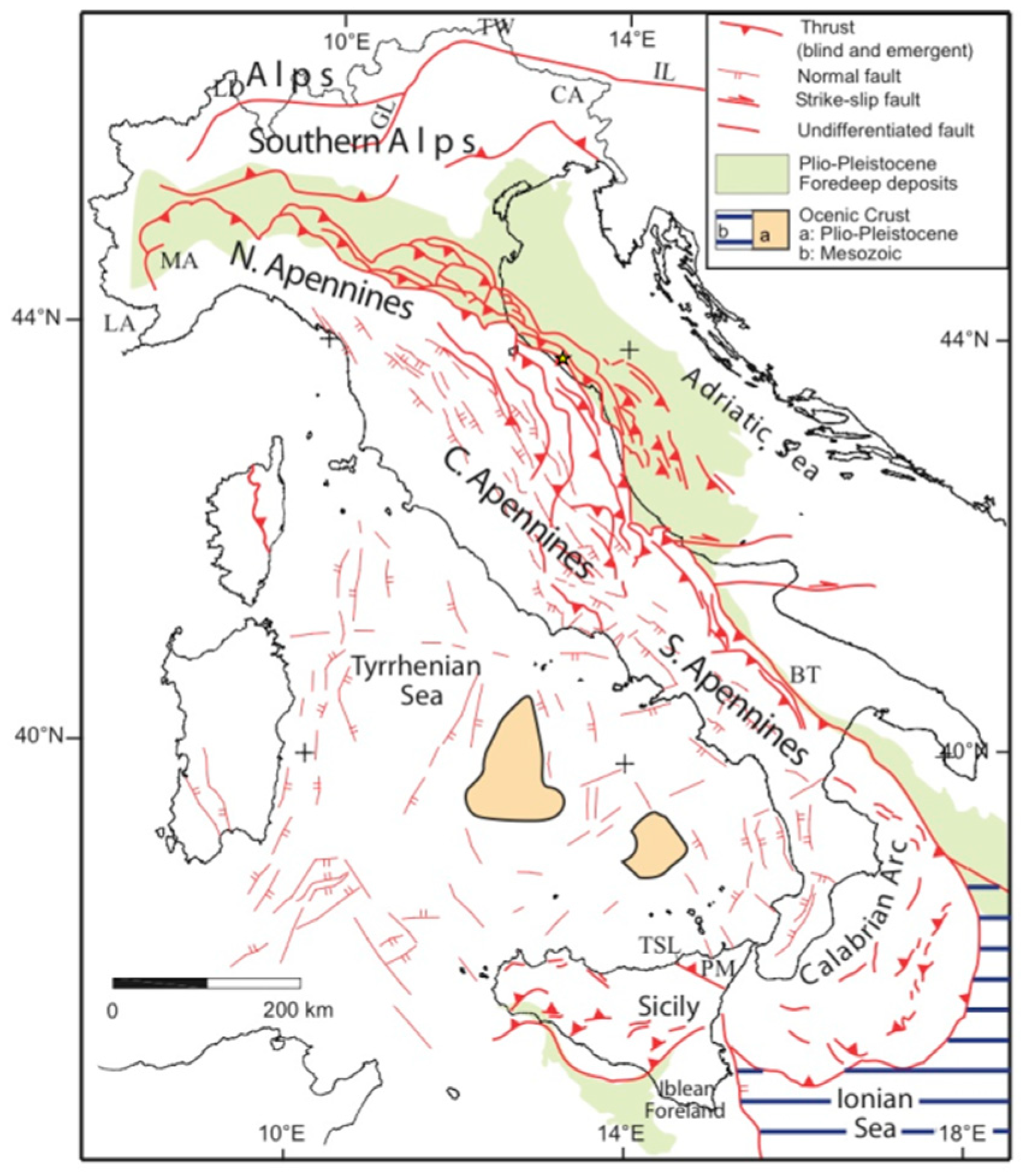
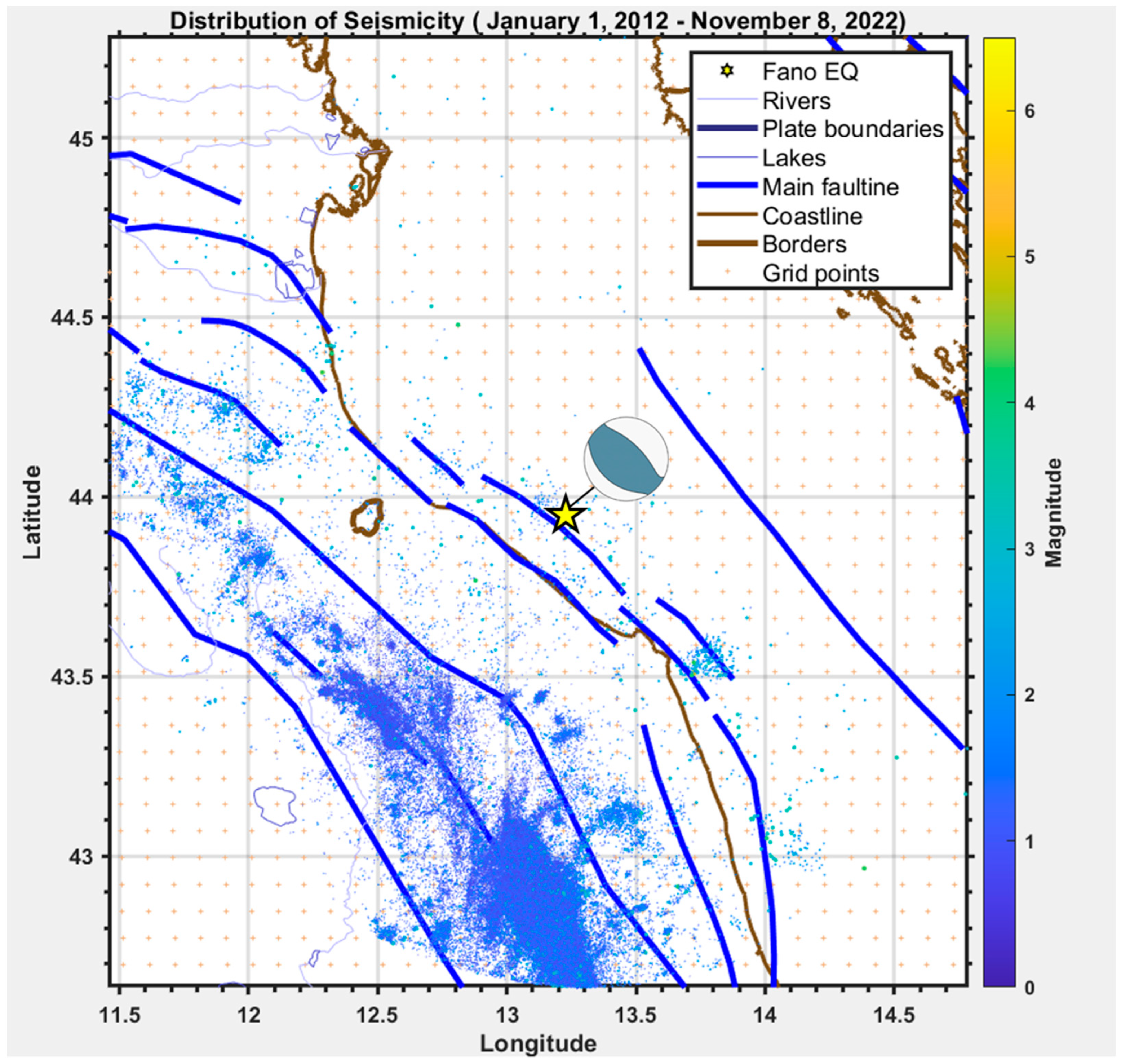
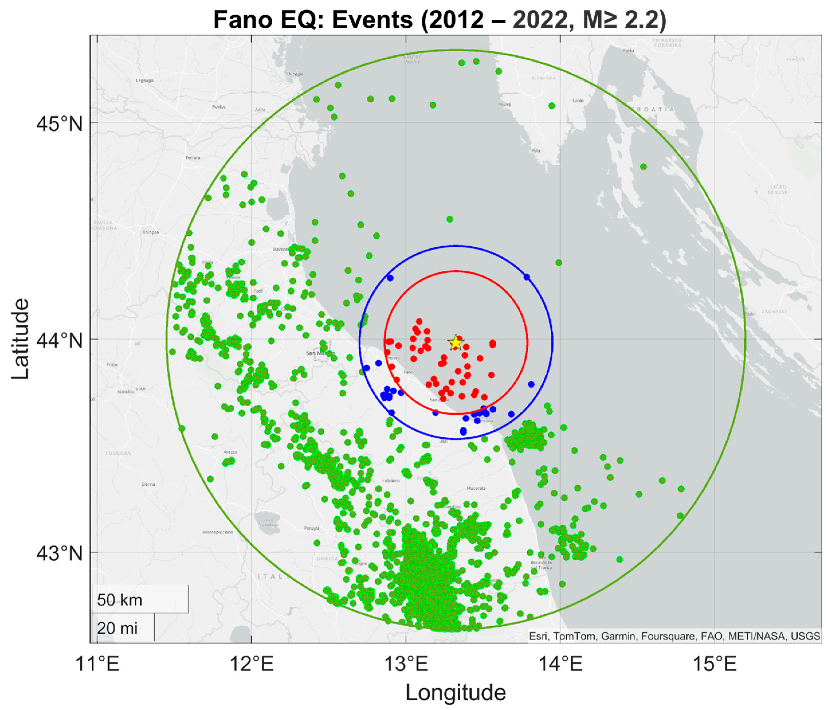
2. Seismotectonic Settings

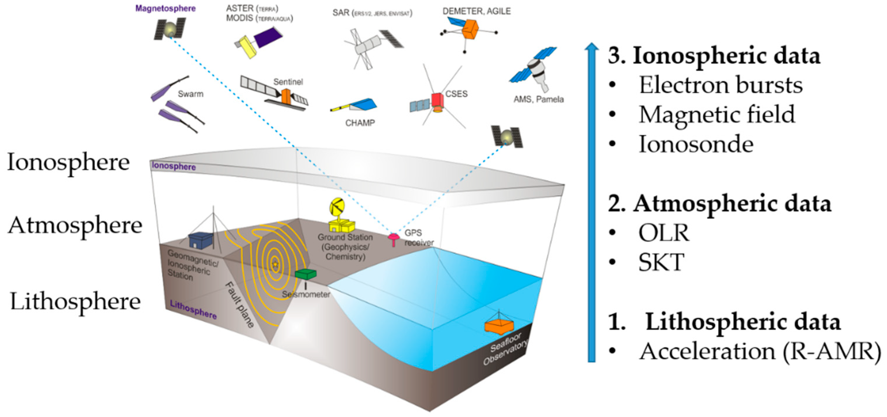
The Adriatic Sea appears as a result of a good variety of structural and stratigraphic processes (Figure 2) guided by fault-related anticlines formed in the Plio–Miocene connected to the main Apennine thrust chain, deeper carbonate structures developed in the south, and a very shallow structure in the Late Pliocene to Quaternary in the central area [32]. During the Mesozoic, this area was affected by an extensional tectonic phase in the Middle Liassic and a compressional paleoinversion in the Lowermost Cretaceous [33,34]. The development of the Alps and the Apennines started from the Middle Eocene onwards in the African continental margin [35,36,37,38,39]. Subsequently, a flexure of the lithosphere belonging to the Adria margin concerned the most internal areas and migrated eastward through time, forming foredeep basins oriented sub-parallel to the belts. The Adriatic domain corresponds to the youngest part of the belt, strictly connected to the evolution of the Apennine fold and thrust belt and to the interaction with the Dinarides, sub-parallel orogenic belts with opposing vergences [32]. In detail, this thrust front is buried beneath Early Pliocene–Quaternary synorogenic deposits.

The entire seismic sequence of November 2022 unfolds along the outermost structure of the Apennine orogeny, characterized by a series of NW–SE trending, NE verging folds forming the easternmost edge of the Apennine thrust front [31,41,42,43]. Over the Tertiary–Quaternary period, this front has gradually migrated towards the east-northeast (e.g., [44]). Geological evidence suggests the ongoing growth of these folds, indicating the continued activity of blind thrust fronts (e.g., [41]).

The presence of historical and instrumental earthquakes with Mw ≥ 5.5, as shown in Figure 3, suggests that thrust faults are also seismogenic [30].

The events recorded on 9 November 2022 represent a manifestation of the ongoing contraction between the Apennine chain, moving towards the northeast, and the Balkan area, which is experiencing a similar but opposite (southwestward) movement. The two hypocenters belong to the blind thrust fault system running parallel to the Marche Coast. This compressive front is located approximately 25–35 km offshore, with a length of about 70 km, and it is referred to as ITCS10 in the Database of Individual Seismogenic Sources (DISS) [41]. This thrust system has therefore been identified as responsible for this seismic sequence (see Figure 3).

3. Data and Methods

To study the effects of LAIC, several datasets are required since each geolayer being investigated demands specific data from various sources. As the analysis is conducted separately in each layer, there are different resolutions both in time and in space, which will be described below.

3.1. Lithospheric Data

From a lithospheric point of view, a seismological analysis was carried out to characterize the seismicity of the area affected by the M_L = 5.7 EQ under inspection, paying particular attention to the area mainly affected by the imminent seismic event. The seismic data provided by the Italian INGV Catalog [47] were used by selecting a circular area with a radius of 150 km around the epicenter and imposing a depth limit of 100 km, covering the period from 1 January 2012 to 8 November 2022 (Figure 4). The temporal and spatial resolutions of the used catalog in terms of earthquake detection (with associated information) are of the order of seconds (or even fractions of a second) and a few km, respectively.

To evaluate R-AMR [48,49], the magnitude completeness (Mc) of the catalog, which represents the minimum value of magnitude for detection, was estimated using the method of maximum curvature [50]. The estimation of Mc was performed as a function of time by sliding time windows, each containing 150 EQs and stepping by five events. The uneven distribution of events within the selected circular area, due to the lack of seismometers on the Adriatic seabed, was taken into consideration. However, the presence of a seismic station located in Banja Luka (Bosnia and Herzegovina), named BLY, allowed for precise event localization. Based on these considerations, an Mc = 2.2 was chosen, resulting in a catalog of 9.099 events. Figure 5 depicts the events (blue and red points) that contributed to the acceleration identified by the R-AMR analysis.

Several studies (e.g., [51,52]) suggested that before significant EQs, there is an accelerated seismic activity under specific conditions. This phenomenon, explained by the Critical Point Theory, likens the main EQ to a phase transition occurring at a “time-to-failure”, $t_f$.

The seismicity preceding the mainshock, often hidden in catalogs, can be revealed through methods like Accelerated Moment Release (AMR), particularly its revised version, known as R-AMR [48,49]. The R-AMR algorithm was applied to EQ data in the Marche region before the Fano EQ. Acceleration in seismicity is measured by examining the accumulation of seismic Benioff strain $s_i=\sqrt{E_i}$, where each event releases strain proportional to the square root of its energy $E_i={10}^{\left(1.5M_i+4.8\right)}$ J. The cumulative strain, $s\left(t\right)=\sum s_i$, is known as Cumulative Benioff Strain. The regional increase in the cumulative Benioff deformation before a large shock is expressed by a power-law time-to-failure functional relation:

$$s\left(t\right)=A+B{\left(t_f-t\right)}^m$$

(1)

where $t_f$ is the time-to-failure (i.e., the occurrence of the mainshock) and m is an inverse measure of how quickly the acceleration grows around $t_f$. To evaluate the quality of seismic acceleration compared to a linear trend representing the background seismicity, Bowman et al. (1998) [51] introduced the C factor, which is the ratio of the sum of the squares of the residuals of the fit of s = s(t) and the same quantity of a linear fit; a C value less than 1 indicates acceleration, with lower values indicating more prominent acceleration. De Santis et al. [48] improved the technique by focusing on strain deposited on the mainshock fault by surrounding seismicity, corrected by a damping function with distance. Cianchini et al. [49] further enhanced the algorithm based on 14 case studies, confirming its ability to reveal hidden acceleration in seismic sequences and provide estimates of $t_f$ and expected magnitude based on parameters A and B of the functional relation. In this analysis, the algorithm is automatic: considering the s = s(t) time series backward and excluding the mainshock, it detects the time when the acceleration starts and the minimum (no attenuation) and maximum circles (with some attenuation). Therefore, for the characterization of seismicity, the R-AMR algorithm was applied to the seismic catalog without taking into account any potential heterogeneity.

3.2. Atmospheric Data

For the atmospheric analyses, data from the ECMWF (European Center for Medium-range Weather Forecasts) ERA5 climatological reanalysis dataset were utilized. This dataset provides comprehensive reanalysis from 1940 up to 5 days prior to the current date, assimilating a wide range of observations in the upper atmosphere and near-surface regions. In our study, however, we focused on parameters dating back to 1980 [53]. This dataset is known for its consistent coverage in both space and time and is minimally affected by observational conditions such as cloud cover in satellite observations. Nighttime values were specifically considered due to their reduced susceptibility to local meteorological changes. Specifically, we analyzed the parameters of SKT and OLR, which are typically reported to be influenced by impending earthquakes. Several studies [54,55,56] have demonstrated how these parameters are directly affected by the “thermodynamic channel” in LAIC models. The ECMWF time series for each atmospheric parameter were collected and pre-processed to apply the Climatological Analysis for Seismic Precursor Identification (CAPRI) algorithm [54,55]. This algorithm compares daily time series of the current year with a historical dataset spanning forty-two years (1980–2021), within a temporal window preceding the seismic event, in our case of 90 days. An anomaly is identified if the observed value persistently exceeds the mean of the historical series by two standard deviations. However, for the current study, anomalies were defined as values exceeding 1.5 standard deviations, considering that the earthquake magnitude was below 6. Additionally, the geographic area investigated was determined based on the circular earthquake preparation region (or Dobrovolsky area) centered on the epicenter [57], resulting in the selection of a geographical area of 2° latitude and 2° longitude.

3.3. Ionospheric Data

To investigate the ionosphere for potential disturbances associated with the Fano EQ, data from ionosonde and satellite sources were analyzed. From the ground, ionosonde measurements can detect the critical frequency of the F2 layer (foF2), the height (hmF2) of the main electron density peak, and also the information of the sporadic E (Es) layer (such as its height, h’Es; its critical frequency, foEs; and the blanketing frequency, fbEs), which can represent the variations of the corresponding layers. Low Earth Orbit (LEO) satellites can detect the in situ plasma parameters and electromagnetic field. The ionospheric station of Rome (43.98° N; 13.32° E) is located 251.44 km from the epicenter, so within the EQ preparation zone according to the formula by Dobrovolsky et al. [57]. Hourly data manually scaled by an experienced operator from the ionograms recorded with the Advanced Ionospheric Sounder (AIS-INGV) [58] were used in this study [59]. Ionospheric anomalies are defined by significant deviations in the parameters h’Es, fbEs, and foF2 compared to a specified background level determined by 27-day hourly running medians centered on the observation day. Specifically, these deviations are calculated according to the following expressions and must satisfy the following criteria, provided they occur within a few hours under geomagnetically quiet conditions specified by daily geomagnetic index values Ap < 9 nT:

$$∆h^{\prime }Es=\left(h^{\prime }Es-{\left(h^{\prime }Es\right)}_{med}\right)\ge 10 \mathrm{k}\mathrm{m}$$

(2)

$$\delta f_{b}Es=\left(f_{b}Es-{\left(f_{b}Es\right)}_{med}\right)/{\left(f_{b}Es\right)}_{med}\ge 0.2$$

(3)

$$\delta f_{o}F2=(f_{o}F2-{\left(f_{o}F2\right)}_{med})/{\left(f_{o}F2\right)}_{med}\ge 0.1$$

(4)

where $∆$ indicates absolute deviations and $\delta$ indicates relative deviations.

The satellite data, on the other hand, are collected by the ESA Swarm three-satellite constellation (Alpha, Bravo, and Charlie). Alpha and Charlie orbit side by side at an altitude of around 460 km, while Bravo orbits at 510 km. Satellite magnetic data have been analyzed using the MASS (MAgnetic Swarm anomaly detection by Spline analysis) methodology for the magnetic data method (see, e.g., [60]). This technique is used to detect electromagnetic anomalies from Swarm magnetic field data (Level 1B, low resolution of 1 Hz) from the analysis of the three components of the geomagnetic field (X, Y, and Z) and intensity (F) for every track of each satellite (Swarm A, Swarm B, and Swarm C) recorded over the EQ preparation area [57]. The analysis consists of the determination of the first differences of the time series (dX/dt, dY/dt, dZ/dt, and dF/dt) and the removal of the long trend using a cubic spline. Moreover, it is important to evaluate the quality of the data using the quality flags provided by ESA, considering only magnetic quiet times (|Dst| ≤ 20 nT and ap ≤ 10 nT) and excluding polar regions (±50° geomagnetic latitudes) because they are very disturbed. After these steps, the root mean square (rms) of sliding windows of 7° shifting every 1.4° was compared with the whole root mean square of the track (RMS). When rms is greater than kt times the value of RMS, the corresponding window is classified as anomalous. For satellite magnetic data, kt is established as 2.5 [60]. This analysis covered a time period ranging from 90 days before the earthquake occurrence to 10 days after and was confined in an area comparable with the EQ preparation region [57].

Since the 1980s, NOAA satellites have continuously circled Earth’s orbit, employing a shared instrument for detecting charged particles since 1998. This instrument, the Medium-Energy Proton and Electron Detector (MEPED), is integrated into NOAA satellites and features eight solid-state detectors meticulously crafted to gauge proton and electron counting rates (CRs) within the 30 keV–200 MeV range with a sampling of 2s [61]. These measurements provide invaluable insights into various phenomena, including radiation belt populations, energetic solar proton events, and the low-energy segment of the galactic cosmic-ray population. Specifically tailored for electron detection, the two telescopes within MEPED delineate three energy bands ranging from 30 keV to 2.5 MeV. The first telescope, angled at 9° towards the local zenith, captures one perspective, while the second telescope, positioned orthogonally at 90° along the satellite’s motion, provides a complementary view. Each compact solid-state detector boasts nominal geometric acceptances of 0.1 cm²sr and opening angle apertures of ±15°.

Statistical correlations between strong EQs and electron bursts (EBs) detected by NOAA were mainly observed considering seismic events around the equator in both the West and East Pacific [62,63]. It was in agreement with the bouncing points of the inner Van Allen Belt (VAB), points where electrons go down close to the earth’s surface, which are also around the equator and cross the ring of fire twice. However, the inner VAB does not generally overhang latitudes above 35°, while mid-latitude EQs are located below the slot region between the internal and external VABs. Seismic events occurring at mid latitudes have therefore apparently minor probability to interact with trapped particles. The representation of a possible interaction scenario between mid-latitude seismic events and trapped electrons is depicted in Figure 6, where the possible area to observe EBs connected to the Fano EQ is shown in pink color. These areas have a longitude range of a few tenths of degrees around those of the seismic event. In fact, the longitude of the seismic event is close to the South Atlantic Anomaly (SAA) border longitude, and the electrons’ mirror points that are far from the SAA longitude will hardly descend to the satellite altitude. Thus, the probability of bouncing electrons to cross the satellite decreases getting away from the SAA. For what concerns the lower latitude EBs, electrons are thought to be coming (direction indicated with pink arrow) from the inner VAB (in yellow), with the interaction (in blue) running along the magnetic field lines. Instead, for what concerns mid–high latitude EBs, electrons are thought to be escaping the trapped conditions (direction indicated with another pink arrow) from the external VAB (still in yellow), with the interaction (still in blue) connecting the two phenomena along the minimum path. The geomagnetic lines (in green) of the internal VAB can cross the lithosphere up to 30°–35° in latitude, so being unlikely to be affected by tectonic activity, whereas the radial propagation of LAIC (in blue) should be able to intercept with greater probability the external belts.

Given the pivotal role of geomagnetic activity in perturbing the ionosphere, instances where the ap and Dst indices exceeded some predefined thresholds were excluded from the ionospheric data analysis. We also verified that no X-class flares occurred during the detected ionospheric anomalies.

4. Results

4.1. Lithospheric Data Analysis

The acceleration of seismicity prior to the mainshock was analyzed by applying the R-AMR method [48,49] to the INGV Catalog, in order to highlight a diverging power-law function over time for the cumulative value of Benioff strain. The focal search area was centered on the epicenter of the event, whose responsible fault system has a length of approximately 70 km [41]. Figure 7 shows the result of the R-AMR analysis, excluding the mainshock and its aftershocks. An evident acceleration is observed, characterized by the C value indicating the onset of “critical” behavior relative to the background, which is 0.598; however, the estimated critical time t_f is 200 days after the mainshock. This accelerated behavior was observed in the fault area within a radius ranging from 0 to 50 km from the epicenter. Additionally, the application of this method provides two expected magnitudes, M(A) = 4.8 and M(B) = 4.7, which, although underestimating the real mainshock magnitude, predict an impending EQ that significantly exceeds the background seismicity. The result of this automatic analysis allows us to place the initial progression of seismic acceleration in the lithosphere around September 2019, i.e., 1155 days before the mainshock, resuming in August 2021, i.e., 455 days before the event. These accelerations are visible from the change in slope in the cumulative curve. Around these dates, it is possible to attempt to identify the establishment of different energy transmission channels towards the ionosphere, as hypothesized in LAIC models.

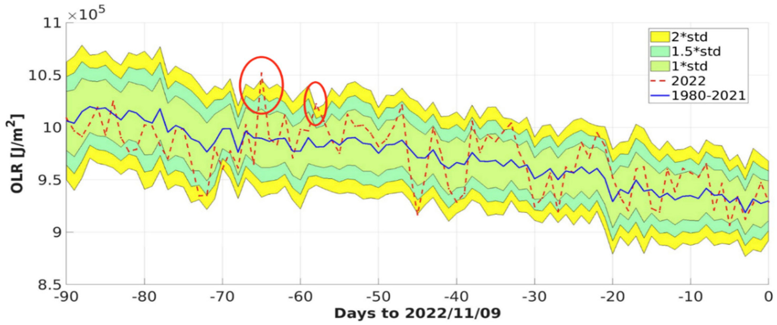
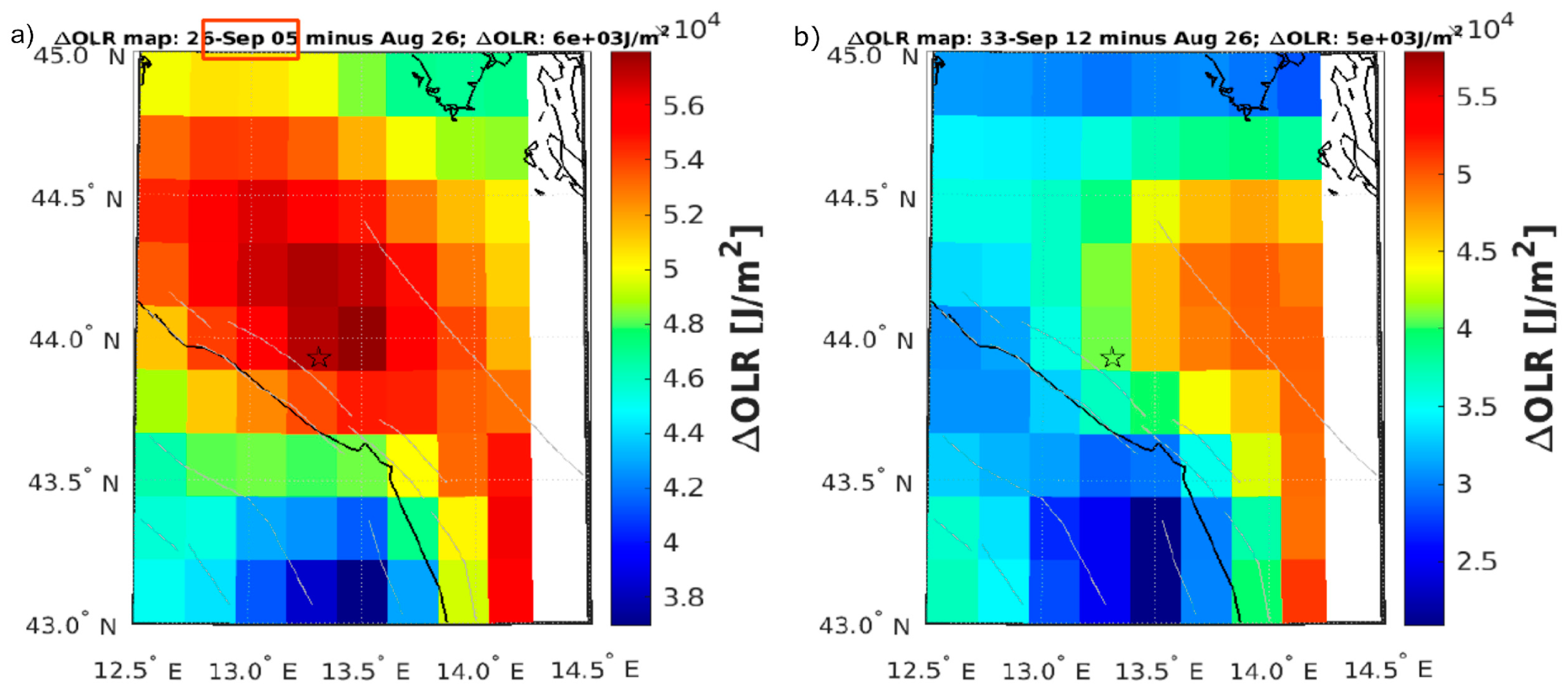
4.2. Atmospheric Data Analysis

SKT and OLR were analyzed to conduct the climatological study. We examined 90 days of ECMWF data preceding the Fano EQ, comparing it with a historical time series spanning the previous 42 years, i.e., from 1980 to 2021. The analysis revealed two highly anomalous days for each atmospheric parameter where the 2022 time series reached the limit of the two standard deviation bands of the historical series. The first anomalous day for SKT occurred on 18 August, i.e., 82 days before the EQ, while the second occurred on 15 September, i.e., 54 days before the EQ (as shown in Figure 8). Furthermore, Figure 9 shows the spatial distribution of these anomalous values, confirming their proximity to the epicenter, especially for the main anomaly. Please note that SKT is defined only on land.

Regarding the OLR parameter, Figure 10 shows two anomalies exceeding the historical mean by two standard deviations on 5 and 12 September 2022, i.e., respectively, 65 and 58 days before the Fano EQ. Interestingly, both anomalies occurred after the first SKT anomaly but before the second one. Figure 11 depicts the spatial distribution of these OLR anomalies, with the first map (a) revealing an extended structure located to the north of the EQ epicenter.

4.3. Ionospheric Data Analysis

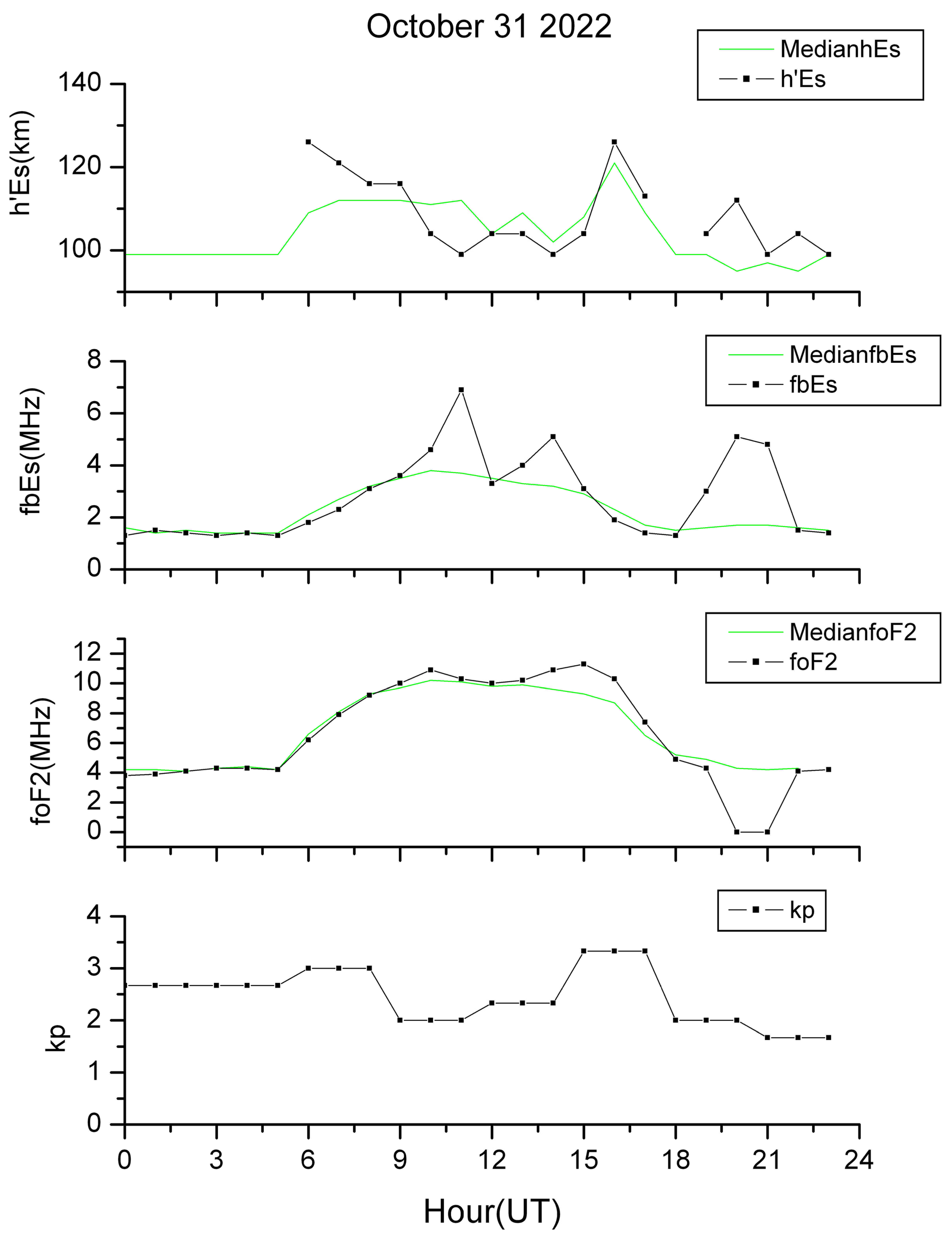
4.3.1. Ionosonde Data Analysis

The application of the ionosonde multiparametric approach [64,65], that takes into account the variations of three ionosonde characteristics, h’Es, fbEs, and foF2, manually scaled from hourly ionograms of the AIS-INGV ionosonde of Rome [66], revealed a single anomaly occurring 9 days prior to the Fano EQ (i.e., on 31 October) at 06:00 UT (

Table 1. Anomaly detected at the ionospheric station of Rome from ionosonde measurements and possibly related to the Fano EQ.

Date	Hour(UT)	Δh’Es	δfbEs	δfoF2	ΔT(Days)	Ap Index	AE Index
31 October 2022	06–07	06–07	0.22	0.21	9	=11 nT	<300 nT

; Figure 12). Since the anomaly occurred on a day with the geomagnetic index Ap = 11 nT, the criterion was not strictly satisfied; however, we preferred to take this anomaly into consideration, given the moderate magnitude of the Fano EQ.

As shown in Figure 13, it is worth noting that the anomaly is consistent with the relationship between ∆T·R and M previously found by the analysis of the most powerful Central Italian EQs since 1984 [66], with ∆T representing the anticipation time (in days), R the distance (in km) between the epicenter and the ionosonde, and M the EQ magnitude.

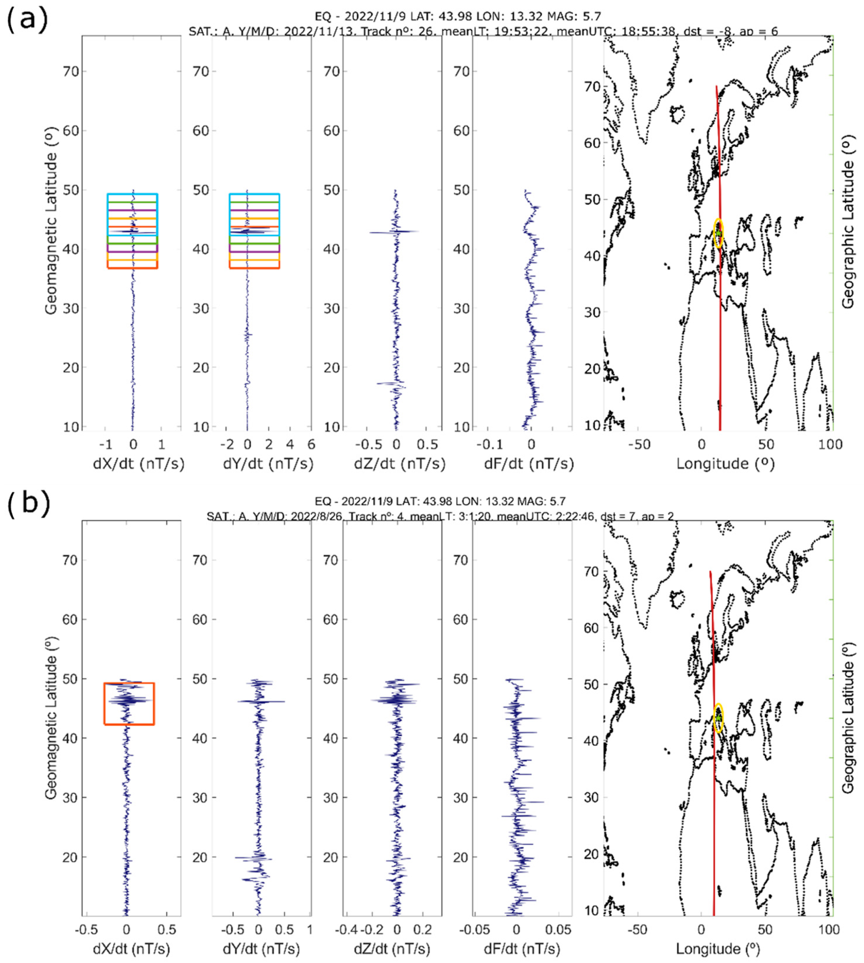
4.3.2. Swarm Satellite Data Analysis

The analysis of satellite magnetic field data from the Swarm constellation has reported two electromagnetic anomalies, which could be correlated with the Fano EQ. Specifically, applying the MASS algorithm to the Swarm A satellite, considering the 90 days before the EQ and 10 days after, an anomaly was detected 4 days after the EQ (Figure 14a), potentially associated with the aftershock period. Another anomaly was also detected 75 days before the EQ, very close to the edge of the analyzed track (Figure 14b).

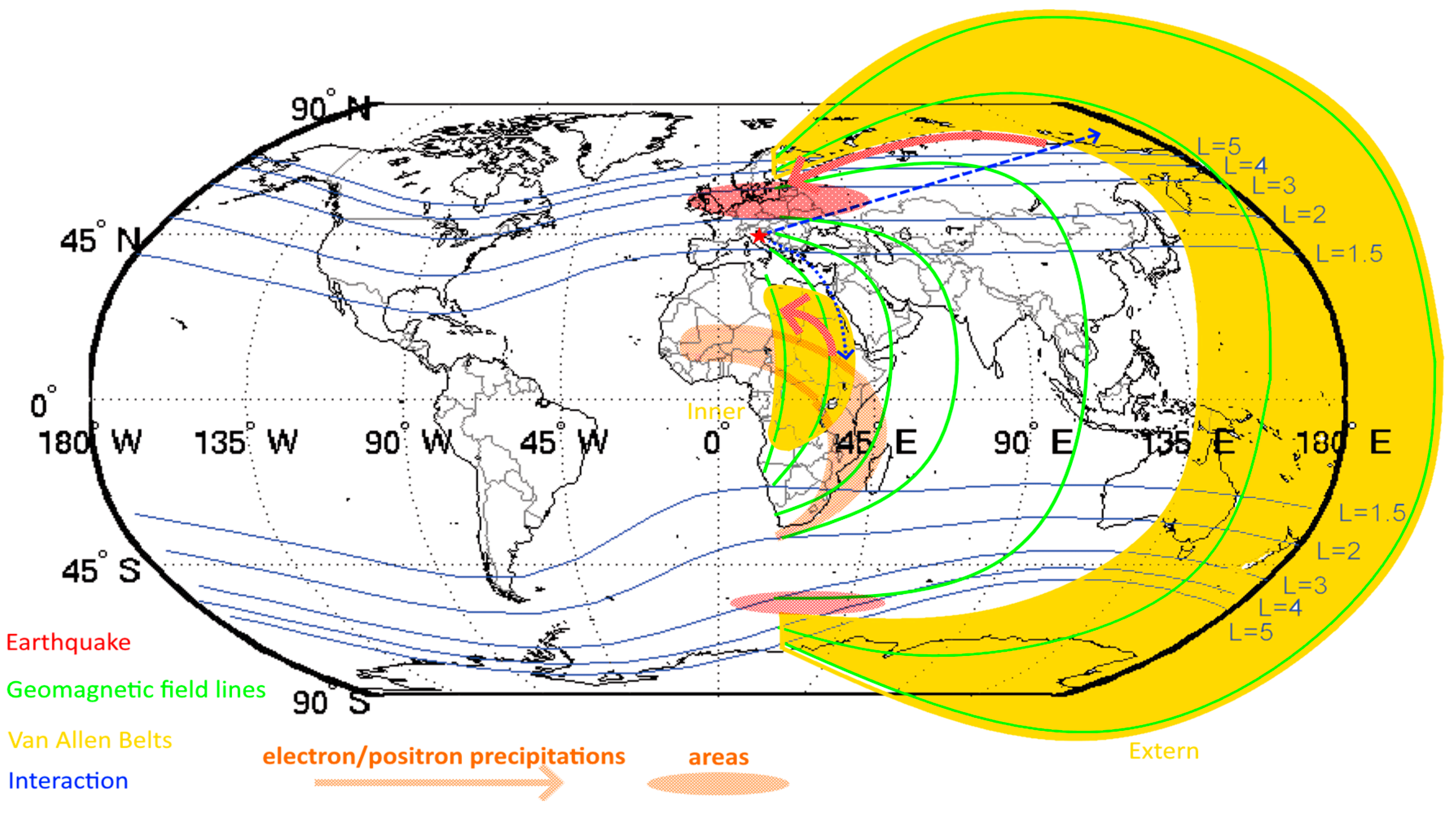
4.3.3. NOAA Satellite Data Analysis: Electron Burst Data Analysis

NOAA electron fluxes were analyzed two days before the EQ and on the event day. Looking at the geomagnetic indices, the geomagnetic activity of these days was quite calm. Then, some candidate EBs were observed over the expected regions. For example, a flux of about 600 electrons cm⁻² s⁻¹ str⁻¹ was observed in the NOAA-15 track on November 8 at a latitude of 50–55° around 20:40 UT, as shown by a red circle in Figure 15. Slight perturbations of around 400 electrons cm⁻² s⁻¹ str⁻¹ were also observed at the previous eastward satellite trajectory, all occurring at around 19:00 UT. Thus, these two perturbations anticipated the Central Italy EQ by 9.5 and 11.2 h, respectively.

5. Discussion

In this paper, precursor anomalies possibly associated with the 2022 M_L = 5.7 Fano EQ (Marche, Italy) were studied using a multiparametric and multilayer approach, including seismic, atmospheric, and ionospheric parameters. The purpose of this multidisciplinary approach is to gather various contributions and connect them to identify the best LAIC model.

Although the resolutions of data are different, we are confident that, when we assimilate them at daily intervals (see

Table 2. List of anomalies detected for the case study of the Fano EQ. From right to left, it shows the analyzed parameter, the day when the anomaly was identified, and the days of occurrence relative to the mainshock. All anomalies appear from bottom (lithosphere) to top (atmosphere and ionosphere). There is only one exception (indicated in bold): a satellite anomaly appears among the atmospheric anomalies.

Parameter	Date	Days to Mainshock
R-AMR	11 September 2019	−1155
R-AMR	11 August 2021	−455
SKT	18 August 2022	−82
Swarm A mag. field	26 August 2022	−75
OLR	05 September 2022	−65
OLR	12 September 2022	−58
SKT	15 September 2022	−54
Ionosonde	31 October 2022	−9
Electron bursts	08 November 2022	−1
Swarm A mag. field	13 November 2022	+4

), we can reconstruct a reliable cumulative number of anomalies. The tracking of the cumulative number of anomalies in chronological order reveals a distinctive behavior, as illustrated in Figure 16.

An exponential fit (indicated by the red curve) accurately represents the overall acceleration of anomalies. This collective progression of anomalies from different geolayers cannot simply be attributed to chance and is probably associated with the preparation phase of the Fano EQ. Furthermore, as highlighted in Table 2, most anomalies appear chronologically from the lithosphere to the atmosphere and ionosphere. This pattern suggests these can be defined as “thermodynamic anomalies”, related to a diffusive–delayed coupling model likely driven by thermodynamic processes. Notably, there is an ionospheric satellite anomaly (indicated in bold in Table 2) amidst the atmospheric anomalies, which could be due to direct electromagnetic coupling between the lithosphere and the ionosphere.

Based on the multiparametric and multilayer analysis, a long-term precursor in the lithosphere was identified. For example, the R-AMR value showed its anomalous acceleration starting about three years before the EQ. From the analysis of atmospheric and ionospheric parameters, anomalies were detected starting 82 days before the Fano EQ. Specifically, the energetic particle signal from NOAA showed an anomaly one day before the seismic event. The Swarm satellites detected an anomaly 75 days before the event and another 4 days after, likely associated with aftershocks. An anomaly was recorded in the ionosonde 9 days before the EQ, and atmospheric anomalies were mainly detected at −82 days and −54 days. The number of anomalies in the atmosphere and ionosphere for this EQ is comparable. This similarity suggests a LAIC behavior of the “thermodynamic” or “diffusive–delayed” coupling, with progression from the lithosphere through the atmosphere to the ionosphere. This progression might correspond to the chemical channel or the acoustic gravity channel, as described in the Hayakawa model [1].

6. Conclusions

In conclusion, this study presents results from the retrospective analysis of the major earthquake that occurred in Italy in November 2022, applying a multiparametric and multilayer approach. This approach involved analyzing data from different geophysical layers (lithosphere, atmosphere, and ionosphere) engaged in the coupling process during the earthquake preparation phase. In the ca. 1200 days preceding the Fano EQ, anomalies appeared primarily from the lowest level (seismic data in the lithosphere) to the higher levels (atmosphere and ionosphere), following an overall acceleration pattern. This confirms that the observed anomalies, which originated during the EQ preparation phase and progressed thermodynamically from the lithosphere to the atmosphere and ionosphere, seem to be consistent with the delayed coupling model. However, the presence of a satellite anomaly between other atmospheric anomalies also seems to confirm the possibility of another direct coupling. Therefore, the overall results would confirm a two-way LAIC model.

References

1. Hayakawa, M. Electromagnetic phenomena associated with earthquakes: A frontier in terrestrial electromagnetic noise environment. Recent Res. Dev. Geophys. 2004, 6, 81–112. [Google Scholar]
2. Freund, F. Pre-earthquake signals: Underlying physical processes. J. Asian Earth Sci. 2011, 41, 383–400. [Google Scholar] [CrossRef]
3. Dahlgren, R.P.; Johnston, M.J.S.; Vanderbilt, V.C.; Nakaba, R.N. Comparison of the Stress-Stimulated Current of Dry and Fluid-Saturated Gabbro Samples. Bull. Seismol. Soc. Am. 2014, 104, 2662–2672. [Google Scholar] [CrossRef]
4. Freund, F. Charge generation and propagation in igneous rock. J. Geodyn. 2002, 33, 543–570. [Google Scholar] [CrossRef]
5. Freund, F. Electric currents streaming out of stressed igneous rocks: A step towards understanding pre-earthquake low frequency EM emissions. Phys. Chem. Earth 2006, 31, 389–396. [Google Scholar] [CrossRef]
6. Freund, F. Pre-earthquake signals, Part I: Deviatoric stresses turn rocks into a source of electric current. Nat. Hazards Earth Syst. Sci. 2007, 7, 535–541. [Google Scholar] [CrossRef]
7. Scoville, J.; Heraud, J.; Freund, F. Pre-earthquake magnetic pulses. Nat. Hazards Earth Syst. Sci. 2015, 15, 1873–1880. [Google Scholar] [CrossRef]
8. Pulinets, S.; Ouzounov, D. Lithosphere–Atmosphere–Ionosphere Coupling (LAIC) model—An unified concept for earthquake precursors validation. J. Southeast Asian Earth Sci. 2011, 41, 371–382. [Google Scholar] [CrossRef]
9. Surkov, V.V.; Pilipenko, V.A.; Silina, A.S. Can Radioactive Emanations in a Seismically Active Region Affect Atmospheric Electricity and the Ionosphere? Izv. Phys. Solid Earth 2022, 58, 297–305. [Google Scholar] [CrossRef]
10. Schekotov, A.; Hayakawa, M.; Potirakis, S.M. Does air ionization by radon cause low-frequency atmospheric electromagnetic earthquake precursors? Nat. Hazards 2021, 106, 701–714. [Google Scholar] [CrossRef]
11. Hayakawa, M.; Molchanov, O.A.; NASDA/UEC Team. Summary report of NASDA’s earthquake remote sensing frontier project. Phys. Chem. Earth 2004, 29, 617–625. [Google Scholar] [CrossRef]
12. Molchanov, O.A.; Hayakawa, M. Seismo Electromagnetics and Related Phenomena: History and Latest Results; Terra Sceintific Publishing: Tokyo, Japan, 2008; Volume 189. [Google Scholar]
13. Korepanov, V.; Hayakawa, M.; Yampolski, Y.; Lizunov, G. AGW as a seismo-ionospheric coupling responsible agent. Phys. Chem. Earth 2009, 34, 485–495. [Google Scholar] [CrossRef]
14. Akhoondzadeh, M. Investigation of the LAIC mechanism of the Haiti earthquake (August 14, 2021) using CSES-01 satellite observations and other earthquake precursors. Adv. Space Res. 2024, 73, 672–684. [Google Scholar] [CrossRef]
15. Sasmal, S.; Chowdhury, S.; Kundu, S.; Politis, D.Z.; Potirakis, S.M.; Balasis, G.; Hayakawa, M.; Chakrabarti, S.K. Pre-seismic irregularities during the 2020 Samos (Greece) earthquake (M = 6.9) as investigated from multi-parameter approach by ground and space-based techniques. Atmosphere 2021, 12, 1059. [Google Scholar] [CrossRef]
16. Nayak, K.; Romero-Andrade, R.; Sharma, G.; Cabanillas Zavala, J.L.; Làopez Urias, C.; Trejo Soto, M.E.; Aggarwal, S.P. A combined approach using b-value and ionospheric GPS-TEC for large earthquake precursor detection: A case study for the Colima earthquake of 7.7 Mw, Mexico. Acta Geod. Geophys. 2023, 58, 515–538. [Google Scholar] [CrossRef]
17. Nayak, K.; Làopez-Uràias, C.; Romero-Andrade, R.; Sharma, G.; Guzmàan-Acevedo, G.M.; Trejo-Soto, M.E. Ionospheric Total Electron Content (TEC) anomalies as earthquake precursors: Unveiling the geophysical connection leading to the 2023 Moroccan 6.8 Mw earthquake. Geoscience 2023, 13, 319. [Google Scholar] [CrossRef]
18. Shah, M.; Calabria Aiber, A.; Arslan Tariq, M.; Ahmed, J.; Ahmed, A. Possible ionosphere and atmosphere precursory analysis related to Mw > 6.0 earthquakes in Japan. Remote Sens. Environ. 2020, 239, 111620. [Google Scholar] [CrossRef]
19. Sharma, G.; Nayak, K.; Romero-Andrade, R.; Mohammed Aslam, M.A.; Sarma, K.K.; Aggarwal, S.P. Low ionosphere density above the earthquake epicenter region of Mw 7.2, El Mayor-Cucapah earthquake evident from dense CORS data. J. Indian Soc. Remote Sens. 2024, 52, 543–555. [Google Scholar] [CrossRef]
20. Tachema, A. Identifying pre-seismic ionospheric disturbances using space geodesy: A case study of the 2011 Lorca earthquake (Mw 5.1), Spain. Earth Sci. Inform. 2024, 17, 2055–2071. [Google Scholar] [CrossRef]
21. De Santis, A.; Cianchini, G.; Marchetti, D.; Piscini, A.; Sabbagh, D.; Perrone, L.; Campuzano, S.A.; Inan, S. A Multiparametric Approach to Study the Preparation Phase of the 2019 M7.1 Ridgecrest (California, United States) Earthquake. Front. Earth Sci. 2020, 8, 40398. [Google Scholar] [CrossRef]
22. Wang, Y.; Ma, W.; Zhao, B.; Yue, C.; Zhu, P.; Yu, C.; Yao, L. Responses to the preparation of the 2021 M7.4 Madoi earthquake in the Lithosphere-Atmosphere-Ionosphere System. Atmosphere 2023, 14, 1315. [Google Scholar] [CrossRef]
23. Akhoondzadeh, M.; Marchetti, D. Study of the preparation phase of Turkey’s powerful earthquake (6 February 2023) by a geophysical multi-parametric fuzzy interference system. Remote Sens. 2023, 15, 2224. [Google Scholar] [CrossRef]
24. Pezzo, G.; Billi, A.; Carminati, E.; Conti, A.; De Gori, P.; Devoti, R.; Lucente, F.P.; Palano, M.; Petracchini, L.; Serpelloni, E.; et al. Seismic source identification of the 9 November 2022 Mw 5.5 offshore Adriatic sea (Italy) earthquake from GNSS data and aftershock relocation. Sci. Rep. 2023, 13, 11474. [Google Scholar] [CrossRef]
25. Grunthal, G. European Macroseismic Scale 1998 (EMS-98). Cahiers du Centre Europeen de Ge´odynamique et de Seismologie 15; Centre Européen de Geodynamique et de Seismologie: Luxembourg, 1998; 99p. [Google Scholar]
26. Tertulliani, A.; Antonucci, A.; Berardi, M.; Borghi, A.; Brunelli, G.; Caracciolo, C.H.; Castellano, C.; D’Amico, V.; Del Mese, S.; Ercolani, E.; et al. (Gruppo Operativo Quest). Rapporto Macrosismico sul Terremoto del 9/11/2022 Della Costa Marchigiana [Data set]. Istituto Nazionale di Geofisica e Vulcanologia (INGV). 2022. Available online: https://quest.ingv.it/rilievi-macrosismici (accessed on 16 May 2024).
27. Maesano, F.E.; Buttinelli, M.; Maffucci, R.; Toscani, G.; Basili, R.; Bonini, L.; Burrato, P.; Fedorik, J.; Fracassi, U.; Panara, Y.; et al. Buried alive: Imaging the 9 November 2022, Mw 5.5 earthquake source on the offshore Adriatic blind thrust front of the Northern Apennines (Italy). Geophys. Res. Lett. 2023, 50, e2022GL102299. [Google Scholar] [CrossRef]
28. Dezi, F.; Merli, A. Chiaradonna A. Soil liquefaction potential of the central Adriatic Coast after the 9th of November 2022 earthquake (Italy). Jpn. Geotech. Soc. Spec. Publ. 2024, 10, 597–602. [Google Scholar] [CrossRef]
29. Montone, P.; Mariucci, M.T. Deep well new data in the area of the 2022 Mw 5.5 earthquake, Adriatic Sea, Italy: In situ stress state and P-velocities. Front. Earth Sci. 2023, 11, 1164929. [Google Scholar] [CrossRef]
30. Console, R.; Vannoli, P.; Carluccio, R. The 2022 Seismic Sequence in the Northern Adriatic Sea and Its Long-Term Simulation. Appl. Sci. 2023, 13, 3746. [Google Scholar] [CrossRef]
31. Vannoli, P.; Basili, R.; Valensise, G. New geomorphic evidence for anticlinal growth driven by blind-thrust faulting along the northern Marche coastal belt (central Italy). J. Seismol. 2004, 8, 297–312. [Google Scholar] [CrossRef]
32. Casero, P.; Bigi, S. Structural setting of the Adriatic basin and the main related petroleum exploration plays. Mar. Pet. Geol. 2013, 42, 135–147. [Google Scholar] [CrossRef]
33. Ziegler, P.A. Compressional Irma plate deformation in the Alpine foreland. Tectonophysics 1987, 137, 420. [Google Scholar]
34. Ziegler, P.A.; Cloetingh, S.; van Wees, J.D. Dynamics of intra-plate compressional deformation: The Alpine foreland and other examples. Tectonophysics 1995, 252, 7–59. [Google Scholar] [CrossRef]
35. Doglioni, C. A proposal for the kinematic modelling of w-dipping subductions—Possible applications to the Tyrrhenian-Apennines system. Terra Nova 1991, 3, 423–434. [Google Scholar] [CrossRef]
36. Bertotti, G.; Picotti, V.; Chilovi, C.; Fantoni, R.; Merlini, S.; Mosconi, A. Neogene to quaternary sedimentary basins in the South Adriatic (Central Mediterranean): Foredeeps and lithospheric buckling. Tectonics 2001, 20, 771–787. [Google Scholar] [CrossRef]
37. Faccenna, C.; Jolivet, L.; Piromallo, C.; Morelli, A. Subduction and the depth of convection in the Mediterranean mantle. J. Geophys. Res. 2003, 108, 2099. [Google Scholar] [CrossRef]
38. Doglioni, C.; Carminati, E.; Cuffaro, M. Simple kinematics of subduction zones. Int. Geol. Rev. 2006, 48, 479–493. [Google Scholar] [CrossRef]
39. Patacca, E.; Scandone, P.; Di Luzio, E.; Cavinato, G.P.; Parotto, M. Structural architecture of the central Apennines. Interpretation of the CROP 11 seismic profile from the Adriatic coast to the orographic divide. Tectonics 2008, 27, TC3006. [Google Scholar] [CrossRef]
40. Consiglio Nazionale delle Ricerche, Structural Model of Italy and Gravity Map; Quaderni de “La Ricerca Scientifica”; Progetto Finalizzato Geodinamica: Roma, Italy, 1992; Volume 3.
41. DISS_Working_Group. Database of Individual Seismogenic Sources (DISS), Version 3.3.0: A Compilation of Potential Sources for Earthquakes Larger Than M 5.5 in Italy and Surrounding Areas; Istituto Nazionale di Geofisica e Vulcanologia: Roma, Italy, 2021.
42. Fantoni, R.; Franciosi, R. Tectono-sedimentary setting of the Po Plain and Adriatic foreland. Rend. Fis. Acc. Lincei 2010, 21, 197–209. [Google Scholar] [CrossRef]
43. Kastelic, V.; Vannoli, P.; Burrato, P.; Fracassi, U.; Tiberti, M.M.; Valensise, G. Seismogenic sources in the Adriatic Domain. Mar. Pet. Geol. 2013, 42, 191–213. [Google Scholar] [CrossRef]
44. Elter, P.; Giglia, G.; Tongiorgi, M.; Trevisan, L. Tensional and Compressional Areas in the Recent (Tortonian to Present) Evolution of the Northern Apennines. Boll. Geofis. Teor. Appl. 1975, 17, 3–18. [Google Scholar]
45. Rovida, A.N.; Locati, M.; Camassi, R.D.; Lolli, B.; Gasperini, P.; Antonucci, A. Catalogo Parametrico dei Terremoti Italiani CPTI15; Versione 4.0; Istituto Nazionale di Geofisica e Vulcanologia (INGV): Roma, Italy, 2022. [Google Scholar]
46. Vannoli, P.; Vannucci, G.; Bernardi, F.; Palombo, B.; Ferrari, G. The source of the 30 October 1930 M w 5.8 Senigallia (Central Italy) earthquake: A convergent solution from instrumental, macroseismic, and geological data. Bull. Seismol. Soc. Am. 2015, 105, 1548–1561. [Google Scholar] [CrossRef]
47. Istituto Nazionale di Geofisica e Vulcanologia (INGV). Earthquake List with Real Time Updates. Available online: https://terremoti.ingv.it/en/ (accessed on 15 January 2024).
48. De Santis, A.; Cianchini, G.; Di Giovambattista, R. Accelerating moment release revisited: Examples of application to Italian seismic sequences. Tectonophysics 2015, 639, 82–98. [Google Scholar] [CrossRef]
49. Cianchini, G.; De Santis, A.; Di Giovambattista, R.; Abbattista, C.; Amoruso, L.; Campuzano, S.A.; Carbone, M.; Cesaroni, C.; De Santis, A.; Marchetti, D.; et al. Revised Accelerated Moment Release Under Test: Fourteen Worldwide Real Case Studies in 2014–2018 and Simulations. Pure Appl. Geophys. 2020, 177, 4057–4087. [Google Scholar] [CrossRef]
50. Wiemer, S.; Wyss, M. Minimum magnitude of complete reporting in earthquake catalogs: Examples from alaska, the western United States, and Japan. Bull. Seismol. Soc. Am. 2000, 90, 859–869. [Google Scholar] [CrossRef]
51. Bowman, D.D.; Ouillon, G.; Sammis, C.G.; Sornette, A.; Sornette, D. An observational test of the critical earthquake concept. J. Geophys. Res. 1998, 103, 24359–24372. [Google Scholar] [CrossRef]
52. Jaume´, S.; Sykes, L.R. Evolving towards a critical point: A review of accelerating seismic moment/energy release prior to large and great earthquakes. Pure Appl. Geophys. 1999, 155, 279–305. [Google Scholar] [CrossRef]
53. Hersbach, H.; Bell, B.; Berrisford, P.; Biavati, G.; Horányi, A.; Muñoz Sabater, J.; Nicolas, J.; Peubey, C.; Radu, R.; Rozum, I.; et al. ERA5 Hourly Data on Single Levels from 1940 to Present; Copernicus Climate Change Service (C3S) Climate Data Store (CDS): Reading, UK, 2018. [Google Scholar] [CrossRef]
54. Piscini, A.; De Santis, A.; Marchetti, D.; Cianchini, G. A Multi-parametric Climatological Approach to Study the 2016 Amatrice–Norcia (Central Italy) Earthquake Preparatory Phase. Pure Appl. Geophys. 2017, 174, 3673–3688. [Google Scholar] [CrossRef]
55. Piscini, A.; Marchetti, D.; De Santis, A. Multi-Parametric Climatological Analysis Associated with Global Significant Volcanic Eruptions During 2002–2017. Pure Appl. Geophys. 2019, 176, 3629–3647. [Google Scholar] [CrossRef]
56. Ouzounov, D.; Liu, D.; Chunli, K.; Cervone, G.; Kafatos, M.; Taylor, P. Outgoing long wave radiation variability 1086 from IR satellite data prior to major earthquakes. Tectonophysics, 2007; 431, 211–220. [Google Scholar] [CrossRef]
57. Dobrovolsky, I.R.; Zubkov, S.I.; Myachkin, V.I. Estimation of the size of earthquake preparation zones. Pure Appl. Geophys. 1979, 117, 1025–1044. [Google Scholar] [CrossRef]
58. Zuccheretti, E.; Tutone, G.; Sciacca, U.; Bianchi, C.; Arokiasamy, B.J. The new AIS-INGV digital ionosonde. Ann. Geophys. 2003, 46, 647–659. [Google Scholar] [CrossRef]
59. Upper Atmosphere Physics and Radiopropagation Working Group; Cossari, A.; Fontana, G.; Marcocci, C.; Pau, S.; Pezzopane, M.; Pica, E.; Zuccheretti, E. Electronic Space Weather Upper Atmosphere Database (eSWua)—HF Validated Data (1.0); Istituto Nazionale di Geofisica e Vulcanologia (INGV): Roma, Italy, 2020.
60. De Santis, A.; Marchetti, D.; Spogli, L.; Cianchini, G.; Pavón-Carrasco, F.J.; De Franceschi, G.; Di Giovambattista, R.; Perrone, L.; Qamili, E.; Cesaroni, C.; et al. Magnetic field and electron density data analysis from Swarm satellites searching for ionospheric effects by great earthquakes: 12 case studies from 2014 to 2016. Atmosphere 2019, 10, 371. [Google Scholar] [CrossRef]
61. Evans, D.S.; Greer, M.S. Polar Orbiting Environmental Satellite Space Environment Monitor—2: Instrument Descriptions and Archive Data Documentation, NOAA Technical Memorandum January; Version 1.4; NOAA National Geophysicial Data Centre: Boulder, CO, USA, 2004; p. 155. Available online: https://ngdc.noaa.gov/stp/satellite/poes/docs/SEM2v1.4b.pdf (accessed on 16 May 2024).
62. Fidani, C. West Pacific Earthquake Forecasting Using NOAA Electron Bursts With Independent LShells and Ground-Based Magnetic Correlations. Front. Earth Sci. 2021, 9, 673105. [Google Scholar] [CrossRef]
63. Fidani, C. The Conditional Probability of Correlating East Pacific Earthquakes with NOAA Electron Bursts. Appl. Sci. 2022, 12, 10528. [Google Scholar] [CrossRef]
64. Perrone, L.; Korsunova, L.P.; Mikhailov, A.V. Ionospheric precursors for crustal earthquakes in Italy. Ann. Geophys. 2010, 28, 941–950. [Google Scholar] [CrossRef]
65. Perrone, L.; De Santis, A.; Abbattista, C.; Alfonsi, L.; Amoruso, L.; Carbone, M.; Cesaroni, C.; Cianchini, G.; De Franceschi, G.; De Santis, A.; et al. Ionospheric Anomalies Detected by Ionosonde and Possibly Related to Crustal Earthquakes in Greece. Ann. Geophys. 2018, 36, 361–371. [Google Scholar] [CrossRef]
66. Ippolito, A.; Perrone, L.; De Santis, A.; Sabbagh, D. Ionosonde Data Analysis in Relation to the 2016 Central Italian Earthquakes. Geosciences 2020, 10, 354. [Google Scholar] [CrossRef]
Figure 1. Summary map of the study conducted: the different layers analyzed are observed, from bottom to top. For each layer, the types of parameters considered are indicated.
Geosciences 14 00191 g001
Figure 2. Simplified structural map of Italy, with the epicenter of the 9 November 2022 Fano EQ indicated by a small yellow star (modified from [40]).
Geosciences 14 00191 g002
Figure 3. Seismotectonic framework of the coastal area of the Marche region. The light blue squares represent the seismic sequence from 9 November 2022 to 14 February 2023; the first event is marked with a yellow star and the second event is shown with a green star. Historical and instrumental earthquakes from CPTI15 [45] are indicated with colored squares, with earthquakes of Mw ≥ 5.5 highlighted in red. The surface projections of seismogenic zones are depicted with orange ribbons [41]. The focal mechanisms of the 9 November 2022 earthquake and the event of 30 October 1930, represented by the grey and white balls, come from TDMT (Time Domain Moment Tensor) and Vannoli et al. [46], respectively (modified from [30]).
Geosciences 14 00191 g003
Figure 4. Spatial distribution of the 174.723 events extracted from the INGV Catalog during the period 2012–2022 within a circular radius of 150 km from the epicenter of the main EQ, highlighted by the yellow star. The grey and white sphere represents the focal mechanism of the earthquake on 9 November 2022. The chosen radius includes the Central Italy sequence (2016), identifiable by the cluster of events to the south near the edge of the area.
Geosciences 14 00191 g004
Figure 5. Spatial distribution of ten years of seismicity around the mainshock, in a radius of 150 km from the epicenter (largest green circle). Blue and red dots (confined within blue and red circles, respectively) represent the events contributing to the acceleration found by the R-AMR analysis. The red dots are the events closer to the seismogenic fault.
Geosciences 14 00191 g005
Figure 6. Scenario of hypothesized pre-EQ coupling processes between the lithosphere of Central Italy and areas where possible EBs could be detected by LEO satellites.
Geosciences 14 00191 g006
Figure 7. Outcome of the R-AMR algorithm applied to the extracted seismic dataset. The red points represent EQs that are closer to the fault (within 37 km) than those represented by the blue points. At the bottom of the main figure, the magnitudes of the involved events are represented: red is used for EQs falling within 37 km from the fault and green those outside that limit.
Geosciences 14 00191 g007
Figure 8. Analysis of the SKT parameter for the Fano EQ with comparison between the 2022 time series (dashed red line) and the historical time series (1980–2021, blue line). Evidenced by red circles there are two quite anomalous values near the second standard deviations from the mean: the first one refers to 18 August, and the second one to 15 September.
Geosciences 14 00191 g008
Figure 9. Maps of the SKT anomalous days in terms of difference with respect to the historical mean: (a) 18 August; (b) 15 September. The EQ epicenter is indicated by the central star. SKT is defined only on land.
Geosciences 14 00191 g009
Figure 10. Analysis of the OLR for the Fano EQ with the identification of two anomalous days that exceed the historical average calculated from 1980 to 2021 by two standard deviations.
Geosciences 14 00191 g010
Figure 11. Maps of OLR anomalous days maps in terms of difference with respect to the historical mean: (a) 5 September; (b) 12 September. The epicenter is indicated by the central star.
Geosciences 14 00191 g011
Figure 12. The anomaly observed 9 days before the 9 November 2022 Fano EQ using Δh’Es, δfbEs, and δfoF2 variations, along with 3 h Kp index values given as a reference of geomagnetic activity.
Geosciences 14 00191 g012
Figure 13. Ionosonde anomaly for the 9 November 2022 M5.7 Fano EQ (red square), compared to the relationship between ∆T·R and M previously found by the analysis of the most powerful Central Italian EQs since 1984 (red line and black squares).
Geosciences 14 00191 g013
Figure 14. Anomalies found 4 days after (a) and 75 days before the Fano EQ (b) by means of an automatic search for magnetic anomalies 90 days before and 10 days after the EQ; MASS algorithm (kt = 2.5) applied to Swarm A satellite. The anomalies are evidenced by coloured rectangles. The vertical red line on the geographical map represents the satellite track.
Geosciences 14 00191 g014
Figure 15. Three-dimensional representation of the NOAA-15 semi-orbits on 8 November 2022; EB evidenced by a red circle while the star identified the EQ epicenter.
Geosciences 14 00191 g015
Figure 16. In a comprehensive approach of the anomalies, the cumulative number of anomalies for Fano EQ is shown here. It is possible to notice that the anomalies appear in time mostly from below (seismic data in the lithosphere) to above (atmosphere and ionosphere). The red curve is an exponential fit of the data.
Geosciences 14 00191 g016