Abstract
The article describes in detail the equipment and method for measuring the Doppler frequency shift (DFS) on an inclined radio path, based on the principle of the phase-locked loop using an SDR receiver for the investigation of seismogenic and man-made disturbances in the ionosphere. During the two M7.8 earthquakes in Nepal (25 April 2015) and Turkey (6 February 2023), a Doppler ionosonde detected co-seismic and pre-seismic effects in the ionosphere, the appearances of which are connected with the various propagation mechanisms of seismogenic disturbance from the lithosphere up to the ionosphere. One day before the earthquake in Nepal and 90 min prior to the main shock, an increase in the intensity of Doppler bursts was detected, which reflected the disturbance of the ionosphere. A channel of geophysical interaction in the system of lithosphere–atmosphere–ionosphere coupling was traced based on the comprehensive monitoring of the DFS of the ionospheric signal, as well as of the flux of gamma rays in subsoil layers of rocks and in the ground-level atmosphere. The concept of lithosphere–atmosphere–ionosphere coupling, where the key role is assigned to ionization of the atmospheric boundary layer, was confirmed by a retrospective analysis of the DFS records of an ionospheric signal made during underground nuclear explosions at the Semipalatinsk test site. A simple formula for reconstructing the velocity profile of the acoustic pulse from a Dopplerogram was obtained, which depends on only two parameters, one of which is the dimension of length and the other the dimension of time. The reconstructed profiles of the acoustic pulses from the two underground nuclear explosions, which reached the height of the reflection point of the sounding radio wave, are presented.
1. Introduction
One of the generally accepted methods for studying the connection between ionospheric disturbances and helio–geophysical processes is the radiophysical method of Doppler sounding of the ionosphere in the shortwave frequency range. The essence of the method is that when a radio wave propagates through the ionosphere, its frequency changes due to the time variability of electron concentration, and the Doppler effect arises. The higher the variation rate of the electron concentration, the larger the observed value of Doppler frequency. An important stage in the development of Doppler observations is associated with the use of publicly available cesium or rubidium frequency standards, which makes it possible to determine the phase and frequency of oscillations with great accuracy. Doppler frequency measurements are taken both with vertical and inclined sounding of the ionosphere. At present, both methods are widely used in studies of the response of the ionosphere to various disturbances.
Doppler frequency measurements on an inclined radio path were carried out for the first time by Essen in 1935, and then they were actively developed in the 1960s [1,2]. Of fundamental importance and impact for further research were the data of Davis and Baker [3] on the possible connection between the disturbances in the atmosphere and ionosphere around the time of the Alaskan earthquake on 28 March 1964. Over the next half-century and beyond, significant progress was made in the study of the state of the ionosphere disturbed by various sources of natural and artificial origin, which is summarized in a number of reviews [4,5,6,7,8,9,10,11,12]. A significant part of the works is devoted to the application of Doppler methods for studying the ionosphere under various helio–geophysical and man-made disturbances [13,14,15,16,17,18].
However, the first studies revealed a number of limitations for the use of the Doppler sounding technique of the ionosphere and showed that, due to the presence of ionospheric heterogeneities, reflected signals arrive at a radio-receiving device in different ways. As a result, a multipath of radio signals is observed, and the problem of interference distortion arises. Measuring Doppler frequencies in multipath conditions is a most difficult issue. In many Doppler installations, spectrum analyzers are required to select individual beams, although using spectrum analyzers, in turn, leads to limitations in the accuracy of measurements of both time and frequency. As is known, the accuracy of spectral analysis depends on the duration of continuous measurement. This is why, for example, to ensure the measurement accuracy of the Doppler frequency shift of 0.01 Hz, a time of about 100 s or more is required. Then, by constructing a time plot of Doppler frequency variations, a detailed description of the disturbances with periods of less than 100 s will be impossible in many cases.
Since the 1970s, the Doppler method of ionospheric sounding has been actively applied for the research of the ionosphere and radio wave propagation in the Ionosphere Sector of the Academy of Sciences of the Kazakh SSR and then at the Institute of Ionosphere of the Republic of Kazakhstan. At first, only vertical sounding was used, and then sounding on an inclined radio path. However, though the accuracy of Doppler frequency measurement with a single-path signal was very high, in the case of the multipath propagation of radio waves, certain difficulties arose in determining the Doppler frequencies and interpreting research results. It was found that the percentage of single-path communication sessions was small, usually 7–9% of their total number, and varied for different radio paths, from 7% to 30% on average [19]. Therefore, the following tasks were assigned by the employers of the Institute of Ionosphere: to ensure the possibility of the continuous registration of the Doppler frequency shift of ionospheric signals, to solve the problem of interference distortions caused by multipath signals, and to increase the accuracy of the measurements.
Further development of the Doppler method at the Institute of Ionosphere was associated with the application of the phase-locked loop (PLL) system. This allowed the registration of the Doppler frequency of a larger-amplitude beam when there is the multipath propagation of radio waves. With this method, the responses of the ionosphere to industrial explosions and underground nuclear explosions have been studied, and the ionospheric effects have been recorded over time intervals from a few tens of seconds to several hours [20,21,22,23,24]. Using the Doppler method with application of PLL has significantly expanded the capabilities of recording ionospheric responses to various natural sources of disturbances, including earthquakes [25,26], volcanic eruptions [27], X-ray and ultraviolet solar flares [28], and the launches of carrier rockets from the cosmodromes “Baikonur” and “Vostochny” [29].
This article describes the method and equipment for measuring the Doppler frequency shift at an inclined sounding of the ionosphere, which is based on the PLL operation principle using a Software-Defined Radio (SDR) receiver. To process the data received and identify the signatures of disturbances, a special program was developed that uses digital filters, correlation, and spectral methods. Then, some examples of the application of the hardware–software complex of Doppler measurements for studying seismogenic disturbances in the ionosphere are considered.
2. The Hardware-Software Complex for Doppler Sounding of the Ionosphere
For the registration of the ionospheric response to disturbances propagating from the lithosphere to the height of the ionosphere, we use the method of Doppler sounding on an inclined radio path with continuous carrier in conjunction with a PLL system and an SDR receiver. The sounding radio wave is reflected from the ionosphere and received by the Doppler radio receiver on the ground with some frequency shift. The receiving Doppler equipment is located in the two measuring points: Institute of Ionosphere (43.17594° N, 76.95342° E) and Radiopolygon Orbita (43.05831° N, 76.97361° E). The measurements of Doppler frequency are carried out on a 13.2 km long low-inclined radio path divided by a mountain ridge, which reduces the passage of the direct radio wave from the transmitter to the Doppler receiver. A special Doppler radio transmitter is used, synchronized by the rubidium frequency standard FE 5650A from “MORION”, INC. (St. Petersburg, Russia).
When measuring the Doppler frequencies on a longer inclined radio path with the length in the range of (200–3000) km, the transmitters of broadcasting stations are employed, as selected from the BBC Short-Wave catalog [30] for different times of day and seasons. The radio paths used in Doppler measurements are listed in Table 1, and the diagram of their relative layout is shown in Figure 1.

Table 1.
The list of radio transmitters whose signals were used for the Doppler sounding of the ionosphere.
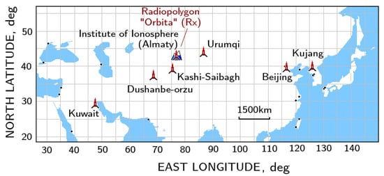
Figure 1.
The disposition scheme of radio transmitters whose signals are used for the Doppler sounding of the ionosphere, relative to the radio receivers (RX) in the points with Doppler installations at the Institute of Ionosphere and Radiopolygon Orbita.
For the measurement of Doppler frequencies in expeditionary mobile conditions, a receiving Doppler installation was developed on the basis of SDR technology. The hardware-software complex provides a round-the-clock monitoring of the shift of Doppler frequency with remote control and access to the data over the Internet.
2.1. The Doppler Receiver
The operation of the receiving Doppler installation utilizes the principle of the PLL based synchronous-phase detector. The main advantages of the application of a PLL are the high sensitivity to small disturbances, the high time resolution, and the ability to operate in multipath conditions which result from the spatiotemporal heterogeneity of the ionosphere and specific propagation features of shortwave radio waves [21].
Previously, in the Doppler installation, we used a radio receiver of the R-399 type, built in accordance with superheterodyne circuitry with a synthesizer-type local oscillator, where a rubidium frequency standard was used as a reference oscillator. At present, with development of the Software-Defined Radio technology [31], a possibility appeared to include an SDR receiver into our Doppler installation instead of the R-399 radio receiver.
The operation principle of SDR is based on the real-time digitization of received radio signal and its further processing in digital form, such that the main treatment of the signal is performed by a computer. A broadband, full-featured 14-bit SDR receiver of RSPdx type [32] covers the radio frequency spectrum from 1 kHz to 2 GHz, providing the spectrum width of up to 10 MHz. The RSPdx receiver operates together with the SDRuno’s own SDRplay software application designed for the Windows operating system. The important condition for the use of the RSPdx receiver in the Doppler installation is the ability to connect to it an external highly stable rubidium frequency standard.
The functional diagram of the receiving part of the Doppler installation based on the SDR receiver is shown in Figure 2. The signal from a highly stable () radio transmitter, after reflection from the ionosphere, arrives via an antenna to the input of the SDR receiver of RSPdx type, which is connected to a computer through the USB port. The SDRuno program, designed for processing the signal from the RSPdx receiver, is set to the CW telegraph signals receiving mode in the band of 150 Hz. As a result, at the output of the computer sound card the signal appears with the frequency of about 1 kHz, which contains the information on the Doppler frequency of the ionospheric signal.
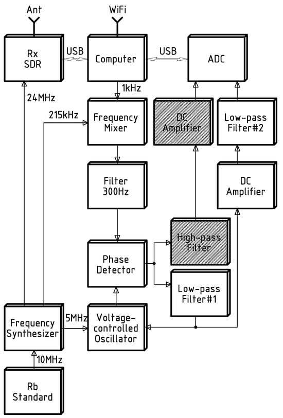
Figure 2.
Functional scheme of the receiving part of the hardware-software complex for measuring the Doppler frequency shift of the ionospheric radio signal using the SDR receiver. See the text for explanations.
Next, a PLL is organized for selection of the Doppler frequency shift of the ionospheric signal. For this purpose, the 1 kHz signal is transferred by a mixer to a frequency of 215 kHz and then, after filtering with a narrow-band electromechanical filter (Filter 300 Hz), it is fed to one of the inputs of a phase detector. The signal of a voltage-controlled oscillator (VCO) comes to the other input of the phase detector. The output signal of the phase detector is connected to a low-pass filter of proportional-integrating type (Filter #1), which determines the parameters of the PLL. This signal acts on the VCO and adjusts it to the frequency of the received signal, such that the change in the voltage at the output of the phase detector is proportional to the Doppler shift. After the passage of a DC amplifier and another low-pass filter (Filter #2), the voltage is digitized by an analogue-to-digital converter (ADC) of E-154 type (L-card, Moscow, Russia), and the results are kept as a file in the computer memory.
The selection principle of the Doppler frequency of a larger-amplitude beam in the case of mutipath signal is described below in Section 2.2.
For remote control, the computer of the Doppler installation is connected to the Internet via a Wi-Fi modem. The on-board time of the computer is synchronized over the network from an NTP server of an atomic frequency and time standard. A special computer program was designed to automate the measurement process, to organize the collection of ADC data, and to visualize the results of the measurement.
The non-linearity of the PLL based conversion of Doppler frequency into voltage was verified by a reference oscillator with hopped adjustment of the output frequency. A highly stable signal was tuned in steps of 0.5 Hz within a frequency range of 5 Hz and fed to the input of the RSPdx receiver. Next, a graph was drawn of the dependence of frequency change on the number of tunings N. As a result, the real transformation characteristic was obtained, denoted as R in Figure 3. The analytic linear approximation of this characteristic looks as .
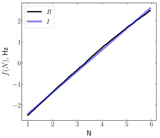
Figure 3.
Comparison of the real characteristic (R) of the PLL conversion of the Doppler equipment with the ideal linear characteristic (I). The units along the horizontal axis are the number N of the succeeding frequency tunings (see text). The plot is taken from the publication Salikhov and Somsikov, 2014 [33].
As it follows from Figure 3, some non-linearity was observed by comparison of the ideally linear characteristic I with the real conversion characteristic R. Within the PLL hold band, Hz, the non-linearity of the real characteristic was less than 1%, and had the value of 0.46%. This is quite sufficient for the high quality measurement of the Doppler frequency shift of the radio signal reflected from the ionosphere in the short-wave frequency range.
2.2. Measuring Doppler Frequencies in Multipath Conditions
As noted above, with single-beam receiving, the accuracy of the Doppler frequency measurement is very high, and is determined only by the frequency instability of reference generator and by the characteristics of ADC equipment. In contrast, by receiving a multipath signal, the interference beats occur between the incoming beams. In dependence on the ratio between the amplitudes of interfering signals, the instantaneous values of frequency spikes can reach tens of Hz, significantly exceeding the Doppler frequencies.
With multipath propagation of radio waves, it is often the case that one of the beams has a higher amplitude than the others. By tracking with a PLL based synchronous-phase detector the behavior of a larger-amplitude beam and averaging its instantaneous values with a low-pass filter, one can quite accurately measure the Doppler frequency of the larger-amplitude beam even in multipath signal.
The measurement accuracy of the Doppler shift of ionospheric signal was determined in the measurements at a special test facility which imitated the conditions of multipath receiving. For the check of the Doppler installation, it was sufficient to use a pair of highly stable oscillators. As shown in Figure 4, two signals from the generators #1 and #2 come, through attenuators, to a frequency mixer, and the interference signal from the mixer output is fed to the input of the PLL-based Doppler equipment. Then, the signal at the output of the PLL is digitized by an ADC and recorded in the computer memory as a text file. The resulting signal of the beating between two frequencies can be simulated with the help of this test facility.
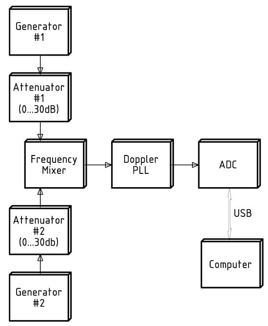
Figure 4.
Schematic of the testing facility to check the operation of the hardware-software complex of Doppler measurements in the imitated conditions of multipath receive.
The signal at the output of the mixer is illustrated by the vector diagram shown in Figure 5, which represents most clearly the physical essence of the phenomenon. As known, on a vector diagram any number of the beams received can be reduced to the two vectors with time-varying amplitude and frequency [19]. With account to this fact, it is sufficient to consider in detail the arrival of only two beams at the input of a radio receiver device. In the simplest case we have the beating of two sinusoids, and , and their resulting oscillation can be determined using the vector diagram of Figure 5. The diagram is built for the case when the circular frequency is higher then , and the amplitude of the beam significantly exceeds that of , .
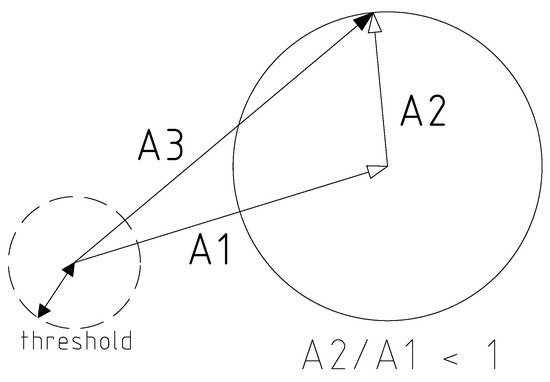
Figure 5.
The vector diagram of the resulting oscillation in a sum of two sinusoidal signals. Designations: —the vector of the larger-amplitude beam, —the vector of the smaller beam, —the resulting vector, which equals to the geometric sum of the vectors and , modulated in phase (frequency) and amplitude by the frequency of the beating.
Let’s suppose that the vector revolves with the frequency together with the drawing plane, such that it remains immovable on the diagram, while the vector rotates with the velocity equal to the circular frequency of the beating, . Then the resulting vector , which represents the geometric sum , turns out to be modulated in its phase (frequency) and amplitude with the frequency of the beating . The frequency of the vector oscillates around the frequency of the larger-amplitude beam () at all values . Consequently, the smaller K, the less the instantaneous value of the resulting frequency differs from the frequency of the beam with the larger amplitude.
In Figure 6 an experimental record is shown of the beating of two signals with different amplitude ratios, , , and , as registered by the Doppler installation at the output of the frequency mixer (see Figure 4). It is seen that in the case of (when the beam is only 15% larger than ), the resulting frequency deviates from the frequency of the larger-amplitude beam and reaches −4 Hz. With the amplitude ratios of and , the deviation of the resulting frequency is significantly lower.
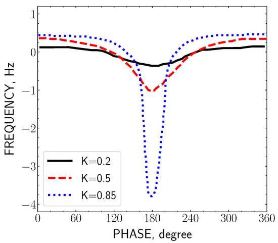
Figure 6.
The change in the resulting frequency, per a cycle of the smaller-amplitude vector , as measured with the different ratios K between the amplitudes of the two sinusoids and .
According to the mathematical analysis of beats [34], in an ideal case the areas under the positive and negative parts of the curves in Figure 6 are equal and opposite in sign. When integrating the oscillations of the difference frequency with a low-pass filter over a single period, a straight line will be obtained coinciding on the graph with the X axis. If the frequency of the beam with larger amplitude varies, the graph obtained after application of integrating filter to the oscillations of difference frequency will repeat the frequency variation of the larger amplitude beam. In the Doppler installation, the averaging of the difference frequency signal proceeds due to the integrating filter (Low-pass Filter #2 in Figure 2). By proper choice of the time constant of this filter, it is possible to adapt the installation to different conditions of multipath receive.
By the conversion of signals in the PLL system, some errors may appear caused both by the operation of electronic devices and the conditions of radio wave propagation. To reveal such errors, the special test measurements were made using the testing facility from Figure 4 with two highly stable generators. One generator was always tuned to the frequency of 5 MHz, the frequency of the other was changed between the limits of 5 MHz + 0.5 Hz and 5 MHz + 7 Hz, which corresponds to the change in the difference frequency from 0.5 Hz to 7 Hz. The parameters of the PLL of the Doppler installation, both the double width of the hold band Hz and the time constant of the low-pass filter s, remained the same throughout entire measuring time.
In Figure 7 a family of curves is shown which demonstrate the dependence of the measurement error of difference frequency for the various ratios K between the amplitudes of the summed signals: , , and . As it follows from this plot, the measurement error of Doppler frequency increases with the rise of the difference frequency . For any value of and Hz, the error always remains below 0.04 Hz. With decreasing K, the value of errors diminishes also, and at the error does not exceed 0.002 Hz. Also, a characteristic segment is seen in the graph of Figure 7, where all curves run parallel to the abscissa axis, and their bend begins at a value of Hz.
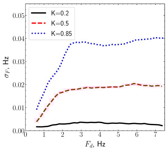
Figure 7.
The measurement error of the difference frequency determined for the various amplitude ratios K.
Therefore, with optimal choice of the PLL double hold band , the accuracy of the Doppler shift measurement with multipath signal can be better than 0.01 Hz, which is 1.5–2 orders of magnitude below the background variations level of the Doppler frequency shift of ionospheric signal.
In Figure 8 an example is shown of the Doppler frequency shift registration by receiving of a real two-beam ionospheric signal on the inclined radio path “Urumqi—Institute of Ionosphere” at a frequency of 9560 kHz. It can be seen there that by selection of the interference signal with the low-pass filter, the Doppler frequency of the larger-amplitude beam was clearly distinguished.

Figure 8.
Receiving a two-beam ionospheric signal by the hardware-software complex of Doppler measurements in realistic conditions. 1—the interfering signal at the output of PLL, 2—the variation of the Doppler shift of the larger amplitude signal selected by the low-pass filter (Filter #2 in Figure 2).
2.3. Registration of Short-Term Ionospheric Bursts in the Records of Doppler Frequency
In the monograph [35] Ya. L. Alpert mentioned the existence of unusual transient ionization flashes which appear and shortly vanish in small regions of the ionosphere. When analyzing the records of the Doppler ionosonde, our attention was drawn by the presence of short-term Doppler bursts with the amplitudes essentially above the background. For further analysis, the detection of such isolated bursts was selected into a special channel of the Doppler installation. A sample of the data recorded in this channel is shown in Figure 9. It was found that the intensity of such bursts was increasing, sometimes considerably, under the influence on the ionosphere of various disturbing factors as, e.g., the sunrise and sunset periods and solar flares. This observation gave the ground to suppose that the intensity of the bursts of Doppler frequency should reflect the state of disturbance of the ionosphere. In this regard, an idea has arisen to measure the intensity of the ionization flashes during Doppler measurements, and the principle of the counting of short-term Doppler bursts was realized at the modification of the PLL based Doppler equipment.
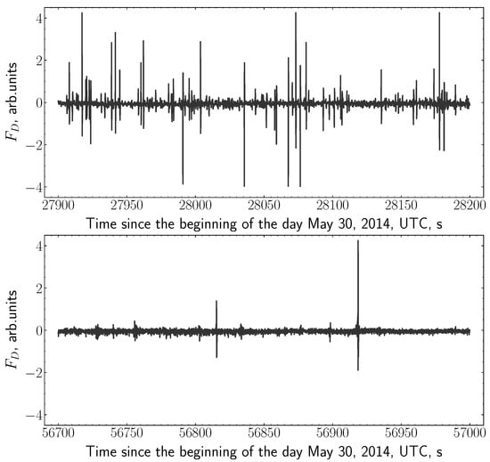
Figure 9.
Two samples of the short-term Doppler bursts reflecting the ionization flashes in the ionosphere. The vertical axis is expressed in the units of Doppler frequency .
For identification of the short-term Doppler bursts, additional units were incorporated into the functional scheme of the hardware-software complex of Doppler measurements: a high-pass frequency filter and a DC amplifier with the regulated gain. In Figure 2 above these two blocks are indicated by hatching. The signal from the output of the phase detector comes to the filter, where its high-frequency component is selected. Then, after amplification, this signal is digitized with a periodicity of 25 Hz by the second ADC channel, and the results are kept in the computer memory. The calculation and graphical visualization of the variations in the intensity of short-term Doppler bursts is made by a specially developed program.
3. Response of the Ionosphere in the Doppler Frequency Shift to Disturbances of Seismogenic Origin
Each strong earthquake presents unique opportunity to study the response of the ionosphere both prior and during the earthquake, and thereby better understand the lithosphere-atmosphere-ionosphere coupling and identify the anomalies which could be used for earthquakes prediction. With the development of the Doppler method of radio sounding of the ionosphere, significant progress was made in the investigation of the ability of acoustic waves to transmit energy from the ground to the uppermost layers of the atmosphere. It was shown that the Doppler method is highly effective for detecting the impact of acoustic waves on the ionosphere even at weak earthquakes and at the earthquakes with the large distance to the epicenter [17,36].
3.1. The Ionospheric Response in the Doppler Frequency Shift to the M7.8 Earthquake in Nepal on 25 April 2015
The M7.8 25 April 2015 earthquake in Nepal occurred at 06:11:23 UTC. The epicenter was located at 28.231° N, 84.731° E, and the depth of its focus was of 8.2 km [37]. The disposition of the hardware-software complex of Doppler measurements relative to the epicenter of the earthquake is presented in the diagram of Figure 10. In these measurements, we used the transmitter of a broadcast radio station in Urumqi, which operated at a frequency of 5960 kHz. The radio receiver of the Doppler installation is placed in the Radiopolygon Orbita point, at a distance of 805 km from the transmitter. The projection of the radio wave reflection point on the ground (sub-ionospheric point) was located at a distance of 1732 km from the epicenter of the earthquake. The Dobrovolsky radius ( km), which determines the size of the zone of deformation processes in the period of earthquake preparation [38], equals to 2259 km for a M7.8 earthquake. Therefore, the monitoring results of Doppler frequency obtained in the said sub-ionospheric point can be used for an objective estimation of the state of the ionosphere at this earthquake.
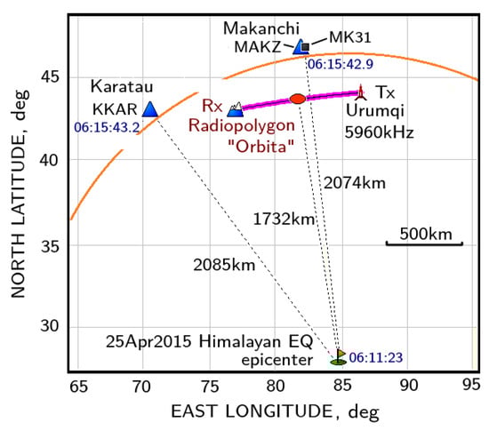
Figure 10.
The disposition scheme of the radio path of Doppler measurements and of the seismic network stations of the National Nuclear Center in Makanchi (MAKZ, MK31) and Karatau (KKAR), in relation to the epicenter of the 25 April 2015 M7.8 earthquake. Tx—the radio transmitter (44.15944° N, 86.89917° E), Rx—the receiver (43.05831° N, 76.97361° E). The red oval indicates the projection of the reflection point of the sounding radio wave (sub-ionospheric point).
An important advantage of Doppler method is its high sensitivity and ability to detect the disturbances in the ionosphere even at considerable distance from an earthquake. Thus, as shown in Figure 11, the seismogenic disturbance from the Nepal earthquake was distinctly observed in the Doppler frequency shift at a distance of 1732 km from the epicenter. The disturbance, with an amplitude above 2 Hz, was detected at 06:28:35 UTC, approximately 17 min (1032 s) after the main shock, and lasted about 91 s.
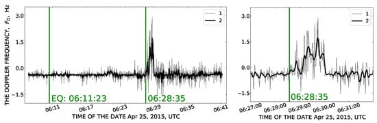
Figure 11.
The response of the ionosphere to the M7.8 earthquake in Nepal on 25 April 2015 registered by the Doppler ionosonde on the “Urumqi—Radiopolygon Orbita ” radio path. 1—the original measurement data; 2—same data after application of the 10 points running average filter.
3.1.1. Determination of the Arrival Time of the Rayleigh Wave to the Sub-Ionospheric Point and the Reflection Height of the Sounding Radio Wave
The acoustic waves generated by the propagation of surface Rayleigh waves cause disturbances in the ionosphere and can be detected by a Doppler ionosonde. The time of response appearing in the Doppler shift record is the sum of the propagation time of the seismic wave to the sub-ionospheric point, plus the time necessary for an acoustic wave to spread from the ground up to the reflection point of the sounding radio wave in the ionosphere.
In the case of the 25 April 2015 Nepal earthquake, no seismic station was situated near the sub-ionospheric point, where the arrival time of the Rayleigh seismic wave could be directly determined. For this purpose, the information was used gained at the closest seismic stations of the National Nuclear Center of the Republic of Kazakhstan: Karatau (KKAR), Makanchi (MAKZ, MK31) and KNDC (Almaty). The data of these stations are accessible at the site [39].
In the seismograms of the vertical Z-component recorded on 25 April 2015 and shown Figure 12, it is clearly seen the successive passage of the Rayleigh wave preceding the appearance of the disturbance in the Doppler shift. It is observed also a certain similarity between the shape of the Doppler shift record and the waveform of the Z-component of seismic wave at the station MAKZ, which was the closest to the sub-ionospheric point.
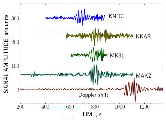
Figure 12.
The fragments of the Doppler shift record and of the seismograms of Z-component written on 25 April 2015 at different distances from the epicenter, at the stations in Makanchi (MAKZ, MK31), Karatau (KKAR), and Almaty (KNDC). The scale of the horizontal axis is expressed in seconds passed since the moment of the earthquake.
The information necessary for the calculation of the speed and arrival time of the Rayleigh wave to the sub-ionospheric point is listed in Table 2. It is seen, that the seismic stations were located at an approximately same distance from the epicenter of the earthquake. The arrival time of the seismic surface wave to the sub-ionospheric point, 630.5 s, was deduced as an arithmetic mean of the indications of nearest seismic stations.
Table 2.
Parameters of the seismological stations used for calculation of the arrival time of the Rayleigh wave to the sub-ionospheric point.
Now, knowing the appearance time of the disturbance in the ionosphere, 1032 s, and the arrival moment of the Rayleigh wave to the sub-ionospheric point, 630.5 s, the time required for an acoustic wave to propagate from the earth’s surface to the reflection point of the sounding radio wave in the ionosphere can be calculated as s.
To determine the propagation trajectory and the reflection height of radio waves, we used the profile of the electron concentration calculated on the basis of the IRI2016 model [40] for the middle point of the radio path, 43.57° N, 81.75° E. The calculation was made directly by the program resided at the model web site [40]. The parameters necessary for the calculation: the index of solar activity and the index of magnetic activity were taken for the date of interest, April 25th, from the sites, correspondingly, [41] and [42].
Then, using the calculated profile of the electron concentration, the path of radio wave propagation was defined by a special program, which took into account the geomagnetic field in accordance with the IGRF13 model for the ordinary component. The result of the calculation is shown in Figure 13, where it is especially indicated the reflection height of the sounding radio wave at 126.0 km.
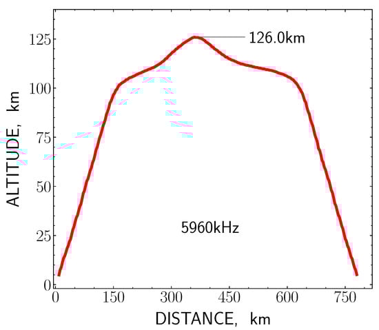
Figure 13.
The propagation trajectory of the sounding wave of Doppler measurements on the radio path “Urumqi—Radiopolygon Orbita ” in the time of the M7.8 Nepal earthquake.
3.1.2. The Propagation Time of Infrasonic Waves to the Reflection Point of the Sounding Radio Wave
In this section, to determine the height in the ionosphere, which an acoustic wave propagating vertically upward from the earth’s surface reaches in 401.5 s, we use the calculation of an altitude profile of the sound speed with account to the viscosity and thermal conductivity of the atmosphere. The calculation method, based on the international atmosphere model NRLMSISE-00, is described in [43,44]. The calculation was made for the coordinates of the sub-ionospheric point in the earthquake time, and for an accepted index of solar activity . The result is shown in the left frame of Figure 14 as a plot of the altitude profile of the sound speed.
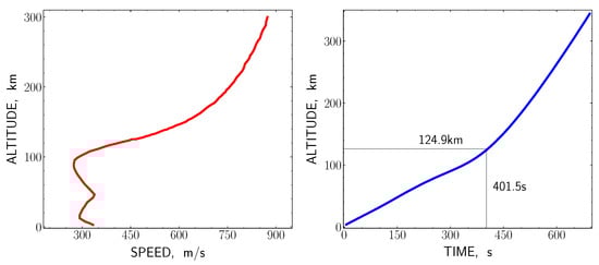
Figure 14.
The estimated altitude profile of the sound speed (left), and the calculated arrival moment of an acoustic wave at the different heights in the ionosphere (right) in the time of the M7.8 Nepal earthquake.
Taking into account the profile of the sound speed, the dependence of the impact time of acoustic wave at the various heights in the ionosphere was calculated, which is presented in the right frame of Figure 14. According to this plot, for the time of 401.5 s the acoustic wave reached a height of 124.9 km, which may be compared with the previous estimation made by the calculation of the trajectory of radio wave propagation—126.0 km. The smallness of the difference between both estimates obtained by the two independent methods, km, indicates a rather good agreement between the experimental and calculated data.
Since geomagnetic storms and substorms induce strong disturbing effect on the ionosphere, taking into account the geomagnetic situation is important for the analysis of seismogenic anomalies in the ionosphere. Note, that during the period from 18 April to 30 April 2015, the geomagnetic situation remained calm, with index below 3. Only on April 21, it was observed for several hours a magnetosphere disturbance with [45]. The -index value during the specified period did not exceed the negative value of nTl, and equaled to nTl on April 25 [42].
Similar co-seismic response of the ionosphere was detected during the catastrophic earthquake in Turkey on 6 February 2023, at a distance of 1591 km from the earthquake epicenter. Monitoring of the Doppler frequency shift was carried out at a frequency of 5860 kHz on the inclined two-hop radio path “Kuwait—Institute of Ionosphere (Almaty)”. The length of the radio path equals to 3010 km, and the distance between the sub-ionospheric point and the earthquake epicenter was 1591 km [26]. As shown in Figure 15, approximately 17 min (998 s) after the main shock, a disturbance was registered in the Doppler shift record, which lasted about 160 s. The double amplitude of the disturbance was more than 2 Hz, which significantly exceeded the background variation of Doppler frequency. The geomagnetic situation during the period from 21 January to 7 February 2023 was calm, such that the Dst-index did not exceed the negative values of nTl, [42]. Just as in the case with M7.8 earthquake in Nepal, the effect observed in the Doppler frequency was a result of the penetration into the ionosphere of the acoustic waves generated by the propagating Rayleigh wave.
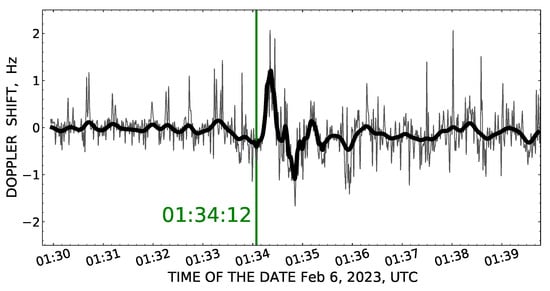
Figure 15.
The response in the Doppler frequency shift of ionospheric signal to the earthquake in Turkey on 6 February 2023, as detected at the radio path “Kuwait—Institute of Ionosphere (Almaty)”. Thin curve—original measurements, bold curve—same data smoothed by a 10 points running average filter. The vertical line indicates the beginning of the ionospheric disturbance in the reflection point of radio waves at 01:34:12 UTC. The plot is taken from the publication Salikhov et al., 2023 [26].
4. The Doppler Observations of Pre-Seismic Disturbances in the Ionosphere before the M7.8 Earthquakes
Taking into account catastrophic consequences of large earthquakes, one of the most pressing issues of modern geophysics is the detection of ionospheric anomalies which could be precursors of seismic events. In recent decades, for investigation of ionospheric anomalies before earthquakes most studies used the data of the Global Navigation Satellite System (GNSS). Thus, intensive studies of seismogenic disturbances in the ionosphere were carried out using the data from the electromagnetic satellites DEMETER and CSES [45,46]. In refs. [47,48,49], brief reviews are given of seismogenic phenomena interpreted as possible precursors of earthquakes, which were recorded in the ionosphere by the ground-based and satellite measurement methods. Up to the present, we have not met any examples of identifying pre-seismic anomalies with application of the Doppler sounding method of the ionosphere.
Short-Term Doppler Bursts before and during the M7.8 Earthquake in Nepal on 25 April 2015
The registration method of short-term Doppler bursts as indicators of ionization flashes was used to study the response of the ionosphere to the earthquake in Nepal and to the preparation process of this catastrophic event.
In Figure 16 the day-to-day records are presented of the variations in the amount of the Doppler bursts. It is seen that the intensity of the bursts significantly increases in the periods of sunrise and sunset, i.e., respectively, around the left and right margin of each plot. During the daytime, the intensity of Doppler bursts remains, as a rule, minimal, provided that the geomagnetic environment is calm and there are no other factors disturbing the ionosphere. In Figure 16 this is clearly seen in the plots built for the days of 25 April 2014 and 15 April 2015.
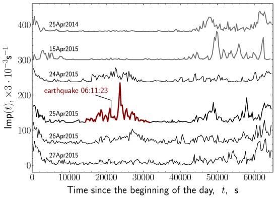
Figure 16.
Intensity of the short-term Doppler bursts detected by the modified method of Doppler measurements before and in the time of the M7.8 Nepal earthquake. The scale of the abscissa axis is expressed in thousands of the seconds passed since the beginning of the day in local time; each distribution covers the time interval of ∼18 h. Along the ordinate axis, the counting rate of short-term Doppler bursts is recorded; the curves are displaced in vertical direction for convenience of comparison.
As noted above, the geomagnetic situation in the period from 18 April to 30 April 2015 was calm. The earthquake occurred at noon, at 12:11:26 of the local time (06:11:26 UTC), which made it possible to register the seismogenic effects in the ionosphere. A noticeable increase in the intensity of Doppler bursts was detected on 24 April, the day before the earthquake, and on 25 April, approximately 90 min before the main shock. The maximum intensity was reached 40 min after the earthquake. Further on, from day to day, the disturbances with decreasing trend were observed at the approximately same time on 26 and 27 April, which is apparently associated with aftershock activity after the earthquake. Thus, the registration of short-term Doppler bursts made it possible to detect the seismogenic disturbances in the ionosphere not only during the earthquake itself, but also in the period of its preparation.
The precursor effects in the ionosphere were also identified at the 6 February 2023 M7.8 earthquake in Turkey. Using the PLL based hardware-software complex of Doppler measurements, the Doppler frequency shift of ionospheric signal was monitored on an inclined, 3010 km long, two-hop radio path “Kuwait— Institute of Ionosphere (Almaty)”. In the variation record of Doppler signal, an expressed increase of the Doppler frequency shift was found, which started approximately 8 days before the main shock, while the maximum values of Doppler frequency were reached at the day of the earthquake [26]. According to the calculated Dobrovolsky radius, the sub-ionospheric point at the first hop of the radio path used was within the limits of the action zone of deformation processes in the lithosphere. This permits to associate the appearance of anomalous effects in the ionosphere with the processes which took place in the lithosphere region of the earthquake preparation.
5. The Lithosphere-Atmosphere-Ionosphere Coupling
5.1. Lithosphere-Atmosphere-Ionosphere Coupling on Example of the M4.2 Earthquake on 30 December 2017
Experimental data on the conjugacy and transmission sequence of seismogenic disturbances in geophysical fields from the lithosphere to the ionospheric heights are of undeniable importance for the study of anomalous phenomena arising at the final stage of earthquake preparation. An important assumption by development of the methods of seismological forecast is the expectation that the preparation process of a strong earthquake should impact, at least, the local geophysical fields. This section presents the examples of ionospheric signatures which have appeared simultaneously with the disturbances in the flux of gamma-rays measured both in the subsoil layers of rock and in the ground-level atmosphere 7 days before a M4.2 earthquake on 30 December 2017.
The measurements of the Doppler frequency shift of ionospheric signal were carried out on a low-inclined radio path between the Institute of Ionosphere (43.17594° N 76.95342° E) and Radiopolygon Orbita (43.05831° N 76.97361° E). The flux of gamma rays, as an exhalation marker of radon and gamma-radioactive products of its decay, was measured at a depth of 40 m inside a borehole, where a gamma detector on the basis of a Ø40 mm NaI(Tl) crystal was installed. Another gamma detector, with a NaI(Tl) crystal of 150 mm in diameter, was placed close to the borehole on the surface of the ground. Both detectors were operating in the continuous monitoring mode. It should be stressed, that the measuring equipment was situated at a distance of only 5.3 km from the epicenter of the earthquake.
On 23 December, seven days before the earthquake, an anomalous intensity outburst of the flux of low-energy, (50–200) keV, gamma rays was registered in the borehole. Presumably, the cause of this effect was a change in the stress-strain state of the rocks before the earthquake, resulting in increased release of radon and its decay products. At the same time, an acoustic microphone with a sensitivity of 25 mV/Pa, also installed in the borehole [50], registered two episodes of the increasing geoacoustic emission, and the thermosensors placed there detected the rising trend of local temperature [25]. As seen in Figure 17, an enhanced level of gamma ray intensity was kept for 3 days, and then during the whole subsequent period until the earthquake.
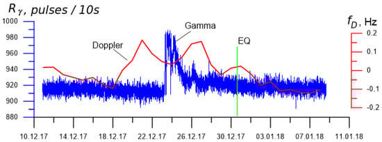
Figure 17.
The outburst of the flux of (50–200) keV gamma rays detected 40 m underground in the borehole prior to the 30 December 2017 M4.2 earthquake, together with the simultaneous negative anomaly in the Doppler frequency shift of ionospheric signal. The moment of the earthquake (EQ) is indicated by a vertical line. The counting rate of gamma rays, , is expressed in the units of the amount of pulses obtained from the gamma detector in 10 s. The data on the Doppler frequency , in Hz, are presented with daily averaging.
In the ground-level atmosphere, an increase of the gamma radiation flux was also observed by the on-ground gamma detector, as illustrated by Figure 18. In this plot, the similar parts in the two records of radiation intensity both above and under the surface of the ground are marked by vertical lines. It is seen that in the ground-level atmosphere the maximum of the radiation flux was reached approximately 5 h later than inside the borehole, which presumably may be stipulated by the sequence of the moving of radioactive substances from the depth of the earth’s crust up to the surface.
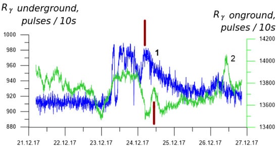
Figure 18.
Comparison of the gamma ray flux variations measured during the period of 22–27 December 2017 at a depth of 40 m in the borehole (1), and at the surface of the ground (2). The counting rates of gamma radiation are expressed as the amount of detector pulses per one second. Two vertical lines mark the mutually corresponding bursts of gamma ray intensity, which were successively appearing, at first in the borehole and then in the ground-level atmosphere.
An advantage of the gamma ray registration 40 m deep in the borehole is the temperature stability, as well as the absence of any influence of atmospheric precipitation to the radiation background. This is why the disturbance in the gamma radiation flux has revealed itself more distinctly in the borehole, so that not only the burst itself was well registered there, but also the fine structure of the response to the earthquake preparation process.
Simultaneously with the appearance of anomalous effects in the borehole, we registered the disturbances in the ionosphere. In Figure 17 it is seen that 7 days before the earthquake a decrease of Doppler frequency occurred, which happened in the time of a sharp increase in the gamma ray intensity. In the day of the earthquake, 30 December 2017, it was also observed small growing in the Doppler frequency shift. It should be noted, that the geomagnetic conditions remained quite at that time, and any geomagnetic storms were absent during the period since 18 until 31 December, which is an important condition for revealing ionospheric response to earthquake preparation.
Thus, our experimental data have shown, that the ionization process of the ground-level atmosphere which occurred during the short-term period of earthquake preparation is an important link in realization of the lithosphere-atmosphere-ionosphere coupling and in appearance of the precursor disturbance in the ionosphere.
5.2. Lithosphere-Atmosphere-Ionosphere Coupling on Example of Underground Nuclear Explosion
In the works of Pulinets et al. [51,52], convincing examples are presented of disturbances appearing in the ionosphere at the growth of the ionization in the boundary layer of the atmosphere, including the cases of underground nuclear explosion. According to the authors, during the underground nuclear explosion in North Korea on 12 February 2013, an earthquake with a magnitude of M4.9 was registered. One hour after the explosion, when a small quantity of radioactive components seeped out onto the surface of the Earth, the GPS satellites registered a negative anomaly in the ionosphere. This observation confirms the concept of the authors, that the burst of ionization may be accompanied by a local increase of atmospheric conductivity, and by a change of electron concentration in the ionosphere above the region with intensified conductivity.
Similar examples of disturbance appearance in the ionosphere at the release of radioactive components of underground nuclear explosion on daytime surface we have observed in 1980th during the tests at the Semipalatinsk test site. To detect the response of the ionosphere, it was used the PLL-based complex of Doppler measurements, and its ability to measure the Doppler frequency shift of a larger amplitude beam was realized [21,53]. In Figure 19 an original record of the Doppler frequency shift is presented, which was obtained at the last underground nuclear explosion on 19 October 1989. The explosion, with a power of 75 kt of TNT equivalent, was executed at 09:50:00 UTC in the borehole #1365 at the Balapan area of the Semipalatinsk test site. The radio-sounding of the ionosphere was proceeding on the radio-path “Kurchatov (50.715° N, 78.621° E)—Sarzhal (49.6° N, 78.683° E)” at a frequency of 7727 kHz.

Figure 19.
Two responses in the Doppler frequency shift of ionospheric signal detected at the 75 kt underground nuclear explosion on 19 October 1989 at the Semipalatinsk test site. 1—510 s after the explosion, 2—1005 s after the explosion. The scale of the horizontal axis is expressed in the seconds passed since the moment of the explosion.
It is seen in the plots, that 510 s (8.5 min) after the explosion a disturbance appears in the record of the Doppler frequency shift of ionospheric signal. This effect is caused by the penetration into the ionosphere of the acoustic waves, the source of which is the movement of the Earth’s surface in the spallation zone (Figure 19, left). Then, 1005 s (16.75 min) after the explosion, another frequency burst is observed, which has an essentially smaller amplitude than that caused by the acoustic impact. From the comparison of experimental records of the Doppler frequency shift it follows, that not only the appearance time, but also the shape and amplitude of the secondary effect differ from the effect connected with the impact of the acoustic waves from the explosion on the ionosphere. As a rule, in our experiments the registration of the Doppler frequency shift proceeded no more than (30–40) min; nevertheless, this occurred sufficient for the detection of the secondary disturbance in the ionosphere. In average, the secondary effects in the records of the Doppler frequency shift of ionospheric signal were registered (15–18) min since explosion.
We noted, that the appearance time of ionospheric anomalies after explosion was comparable with the time of radioactivity enhancement in the atmosphere as revealed by direct measurements of the radioactive background in the atmosphere from helicopters and planes [54,55]. Thus, on 19 October 1989, in the borehole #1365 an exit of the products of nuclear explosion onto the ground surface was observed, with a rise of radioactive background up to (15–40) R/h in the epicenter zone [56]. According to statistics, explosions of incomplete camouflage accompanied by the small exhalation of radioactive gases composed a 45% share of the whole number of tests at the Semipalatinsk site [55], and 67% of the tests at the Novaya Zemlya site [54]. The practice of the tests at the Arctic nuclear polygon shows, that by all camouflage nuclear explosions an escape of radioactive products of underground explosion onto the surface occurred, as a result of filtration through the zones of melting, crushing, micro- and macro-fissuring. If the release happened less than one minute after the explosion, the isotopes Sr-89, Sr-90, Ba-140, Cs-137 were detected in the atmosphere. If the time delay between the explosion and the gas exit was above one, but below 33 min, the isotopes Sr-89 and Cs-137 were detected, and after 33 min only Cs-137 remained.
As a result of the seismic impact of the energy of nuclear explosion on rock massif, large masses of natural Rn, Th and their daughter products are also thrown out into the atmosphere [54]. The ingress of radionuclides in the atmosphere leads to ionization of its ground-level layer, which may be one of the links of disturbance transmission in the lithosphere-atmosphere-ionosphere system.
According to modern concepts, the key factor of anomalies generation in the ionosphere is the change in the conductivity of the atmospheric boundary layer and the complex of physical and chemical processes proceeding under the influence of ionization [52,57]. Then, the appearance of anomalous effects in the ionosphere both after an underground nuclear explosion and in the short-term period of earthquake preparation can be explained on the basis of a general mechanism consisting of the processes which take place at the ionization stage of the ground-level atmosphere. In the case of an underground nuclear explosion, the exit of radioactive substances occurs after explosion, while by earthquakes the ionization of the near-earth atmosphere, as an exhalation result of radon, thoron, and their daughter products, is detected before the main shock.
Experimental records of the response of the ionosphere to underground nuclear explosions were a basis for an estimation of the velocity profile of an acoustic pulse by the Doppler frequency shift of the sounding radio wave.
6. A Simple Formula for Estimating the Profile of an Acoustic Pulse Velocity by the Doppler Shift of the Frequency of Sounding Radio Wave
In this section, a possibility is considered to restore the profile of the acoustic pulses which have reached the reflection point of radio waves in the ionosphere from the two underground nuclear explosions. In principle, such formula can be only derived under exclusive conditions of a powerful acoustic impact on the ionosphere, and on the basis of reliable data of Doppler sounding.
It should be noted, that proceeding of any direct acoustic observations at the height of upper atmosphere (ionosphere) seems impossible. This is why we turned to an analysis of the historical records of the Doppler frequency shift obtained by the Doppler method using PLL, the effectiveness of which was demonstrated during underground nuclear explosions at the Semipalatinsk test site. Measuring the Doppler frequency shift by the short-wave radio sounding of the ionosphere is a widely used instrument for studying the disturbances in the thermosphere of both natural and artificial origin. Usually, the Doppler frequency shift is calculated in the approximation of geometric optics, and its value is determined by the rate with which the electron concentration changes in time along the trajectory of radio beam [58].
Here, a simple formula is obtained which allows to acquire a good estimate for the relationship between the velocity field of acoustic disturbances and the measured Doppler frequency. The results obtained may be a reference point in the development of numerical models of the propagation of an acoustic pulse from an underground nuclear explosion into the upper layers of atmosphere.
Under disturbances that do not affect the ionization balance, the change in electron concentration over time is entirely determined by the velocity field of the charged component. The velocity of the charged component can be related to the velocity of the neutral gas and, as a result, the Doppler frequency shift can be represented as a functional of the velocity field of the neutral component of the ionospheric plasma. This representation is convenient, since calculating the Doppler shift no longer requires preliminary labor-intensive reconstruction of the electron density profile from the field of disturbance velocities.
For the acoustic disturbances, the characteristic spatial size of which exceeds the size of the region of significant interaction of the radio wave with the ionospheric plasma, it is possible to analytically invert the expression for the Doppler frequency shift, and to obtain a fairly simple formula for the velocity of the neutral gas, suitable for practical processing of Dopplergrams.
In the isotropic case, the phase of the radio wave at the receiving point relative to the transmission point is given by integrating the refractive index along the radio beam trajectory
where is the circular frequency of the sounding radio wave; c is the speed of light. By virtue of Fermat’s principle:
the perturbation of the radio wave phase corresponding to the perturbation of the refractive index can be expressed, accurate to linear terms, by an integral along an unperturbed trajectory
This leads to the determination of the Doppler frequency shift [58]:
where is the disturbance of the electron density; is an element of the length along the trajectory. Using the linearized continuity equation
the rate of change in the electron concentration can be expressed in terms of the velocity field of the charged component of the plasma. As a result, we get:
where is the height vector of the homogeneous ionosphere. The equations for the change along the trajectory of the wave vector of a radio wave ,
allow us to express the Doppler frequency shift (4) through the parameters of the unperturbed trajectory
Under the magnetization conditions of plasma ions, the charged component is entrained by the neutral component only along the geomagnetic field
where is the perturbation of the velocity field of the neutral component, is the induction of the magnetic field. Formulas (8) and (9) make it possible to efficiently calculate the magnitude of the Doppler frequency shift in the numerical simulation of the unperturbed beam trajectory , , which occurs due to the motion of the neutral component of the ionospheric plasma. A noticeable change in the wave vector of the radio wave, and consequently the contribution to the integral (8), occurs only in the regions of significant interaction of the radio wave with the ionospheric plasma. Usually, it is sufficient to consider a small neighborhood of the reflection point as such an area.
If the characteristic spatial scale of the acoustic disturbance exceeds the size of the region of significant interaction of the radio wave with the ionospheric plasma, the integral (8) can be approximated by the first terms of its asymptotic expansion at . To do this, following the usual method of obtaining asymptotic expansions of this kind of integrals, we decompose the integral expression into the Taylor series at the reflection point , and the integration region is limited to the section of the radio beam trajectory in the interval of altitudes from to . In this region, the change in the wave vector of the sounding radio wave constitutes a ∼0.8 share of its complete change.
where
where is the altitude of the reflection point; is the initial value of the angle between the wave vector and the vertical; , are the values of x-coordinates on the ascending and descending branches of the trajectory. The numerical values of the quantities are obtained by approximating the electron concentration profile in the vicinity of the reflection point by the exponent . For Formula (10) to be applicable, it is necessary that the vertical linearity of the velocity profile was not less than , and the horizontal dimension was not less than .
Let us consider the problem of the Doppler frequency shift caused by the disturbance from an acoustic wave. We approximate the velocity field of the neutral component in the vicinity of the reflection point of sounding radio wave by a longitudinal pulse propagating with the local sound velocity and with exponential change of the amplitude with altitude. The vector is directed vertically upwards.
By differentiating (14), we obtain the evolutionary equation for each of the components of :
Let us express, with the help of (15), the spatial derivatives of the velocity field in terms of temporal ones, for example:
By substituting (16) into (10) and neglecting the second derivative of time, we get the final formula:
where
, , are the angles between the magnetic field and the direction of acoustic pulse propagation, the magnetic field and the vertical, the direction of acoustic pulse propagation and the vertical; H is the height of the homogeneous atmosphere at the reflection point; is the speed of sound at the reflection point. When , formula (17) turns into the formula for the Doppler frequency shift for a radio wave reflected from a moving mirror, which is often used for estimates (though not always justified).
Formula (17) gives a solution to the problem of determining the Doppler frequency shift from the time profile of the velocity of wave disturbance in the neutral gas at the reflection point of radio wave. In addition, it is not difficult to reverse the formula by solving differential equation, and thereby to solve the inverse problem of determining the velocity profile from the measured Doppler frequency shift. The treatment will be unambiguous if the physically necessary conditions of boundedness are imposed on the velocity disturbance,
since Equation (17) for at has no non-zero bounded solutions. From (17) and (21), taking into account the relation , the desired inversion formula follows (it is assumed that ):
Let us dwell in more detail on the case when the Doppler frequency shift occurs only starting from the zero moment of time:
In this case, as follows from (22),
From (24) we conclude that if the acoustic pulse is non-zero in the interval , then it must have a leading edge of a special shape (, ). In a real experiment, such situation can only arise if additional measures were taken. We do not consider this option, so we believe that . Thus, Dopplerograms that originate at must satisfy the condition
Equation (25) can be used to adjust the parameter T if the available ionospheric data is insufficiently reliable.
Our Equation (22) for reconstructing the velocity profile of an acoustic pulse depends on only two parameters: , which has the dimension of length, and T, which has the dimension of time. If we set the parameter T equal to zero, we arrive at the case of the reflection of radio wave from a moving mirror, which is often used to estimate the velocity profile of disturbance. It is important to note, that in this case, the restoring error of the velocity profile can distort the result several times and distort the shape of the profile.
Figure 20 and Figure 21 show the records of the Doppler frequency shift and reconstructed velocity profiles in the reflection point of sounding radio wave for the two acoustic pulses which were propagating from the underground nuclear explosions carried out at the Semipalatinsk nuclear test site on 17 December 1988 and 19 October 1989.
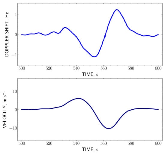
Figure 20.
The record of the Doppler shift measured at the underground nuclear explosion on 17 December 1988, and the restored velocity profile . The frequency of the sounding radio wave MHz, the altitude of the reflection point km, m, s.
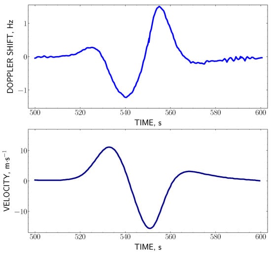
Figure 21.
The record of the Doppler shift measured at the underground nuclear explosion on 19 October 1988, and the restored velocity profile . The frequency of the sounding radio wave MHz, the altitude of the reflection point km, m, s.
The obtained results can serve as a reference point in development of the numerical propagation models of the acoustic pulses which arise in the upper layers of the atmosphere from underground nuclear explosions.
7. Conclusions
The article describes in detail the method and equipment for measuring the Doppler frequency shift by inclined sounding of the ionosphere on the basis of PLL operation principle. The task was to expand the capabilities of the Doppler method for registration of the ionospheric response to seismogenic and anthropogenic impacts, and to detect the appearance of pre-seismic signatures in the ionosphere prior to large earthquakes. As a result, it became possible to register continuously, with good accuracy and reliability, both the Doppler frequency shift and the short-term Doppler bursts which reflect disturbances in the ionosphere.
- Application of an SDR receiver using the digital technology of Software-Defined Radio in the Doppler installation ensured the high characteristics of the radio receiving tract.
- The use of the PLL system permitted to carry out the continuous measurement of Doppler frequency and to measure the Doppler frequency shift of larger-amplitude beam under multipath conditions; this is an evident advantage of the considered method.
- With an optimal choice of the PLL hold band, it was achieved an accuracy of ⩽0.01 Hz in the measurement of Doppler frequency shift, which is 1.5–2 orders of magnitude below the background variations of Doppler frequency in the F-region of the ionosphere.
- A modification of the Doppler installation was made for the registration of short-term ionization bursts in the ionosphere. For this purpose, two additional blocks were included into the functional scheme of the Doppler installation: the high-pass filter and DC amplifier, a separate channel of signal digitization was organized, and a special program was developed for operation of the data obtained.
The radiophysical method of Doppler sounding of the ionosphere using PLL was applied for investigation of seismogenic and artificial disturbances in the ionosphere. During the two M7.8 earthquakes, in Nepal (25 April 2015) and Turkey (6 February 2023), the pre- and co-seismic effects in the ionosphere were revealed, the appearance of which relates to different propagation mechanisms of seismogenic disturbance from the lithosphere up to height of the ionosphere.
- The co-seismic effects, which arose as a result of the penetration into the ionosphere of the acoustic waves caused by propagation of Rayleigh wave, were detected by the Doppler ionosonde at a distance of 1732 km from the epicenter of Nepal earthquake, and at 1591 km from the epicenter of the earthquake in Turkey.
- Pre-seismic effects, as noticeable increase in the intensity of Doppler bursts reflecting the disturbance state of the ionosphere, were registered one day before the earthquake in Nepal, as well as 90 min prior to the main shock. The intensity of Doppler bursts had a constant rising trend, and its maximum was achieved 40 min after the earthquake.
- A pre-seismic effect in the ionosphere, as noticeable increase of the Doppler frequency shift, was detected in the records of Doppler frequency 8 and 3 days before the earthquake in Turkey, and the maximum value of Doppler frequency was achieved on the day of the earthquake.
- A channel of geophysical interaction in the system of lithosphere-atmosphere-ionosphere coupling was traced, when 7 days before a M4.2 earthquake the disturbances in the ionosphere were detected simultaneously with an intensity increase of the flux of gamma-rays both in the borehole, under the surface of the ground, and in the ground-level atmosphere, which resulted in the ionization of the ground-level atmosphere.
- The concept of lithosphere-atmosphere-ionosphere coupling, where the key role is assigned to the ionization of the atmospheric boundary layer, found confirmation in an retrospective analysis of the records of Doppler frequency shift of ionospheric signal made during the underground nuclear explosions at the Semipalatinsk test site in the late 1980s. It was established, that after nuclear explosion the Doppler ionosonde registered first the distinct penetration signature of an acoustic wave into the ionosphere, then a disturbance in the ionosphere coinciding with the rise of radioactivity in the atmospheric boundary layer.
- A simple formula for reconstructing the velocity profile of an acoustic pulse from Dopplerogram was obtained, which depends on only two parameters, one of which has the dimension of length, and the other the dimension of time. The article presents the reconstructed profiles of the acoustic pulses from the two underground nuclear explosions, on 17 December 1988 and 19 October 1989, which have reached the reflection points of sounding radio wave in the ionosphere.
Author Contributions
Conceptualization, N.S.; methodology, N.S. and V.S.; software, N.S. and A.S.; formal analysis, N.S., V.S. and G.P.; data curation, N.S. and A.S.; writing—original draft preparation, N.S., G.P. and V.S.; writing—review and editing, N.S., V.S., G.P., S.N. and A.S.; project administration, N.S., S.N., V.R. and V.Z.; funding acquisition, N.S. and S.N. All authors have read and agreed to the published version of the manuscript.
Funding
1. This research was funded by the Science Committee of the Ministry of Science and Higher Education of the Republic of Kazakhstan, grant number AP19678127 ”Development of the methods for geophysical fields monitoring in the lithosphere-atmosphere-ionosphere-magnetosphere system in a seismically hazardous region of Northern Tien Shan”. 2. This research was funded by the Science Committee of the Ministry of Science and Higher Education of the Republic of Kazakhstan, grant number BR20280979 “Comprehensive study of the impact of the solar origin sources on the near-Earth space state”.
Data Availability Statement
The data presented in this study are available on request from the corresponding author.
Conflicts of Interest
The authors declare no conflicts of interest.
References
- Watts, J.M.; Davies, K. Rapid frequency analysis of fading radio signals. J. Geophys. Res. 1960, 65, 2295–2301. [Google Scholar] [CrossRef]
- Davies, K.; Watts, J.M.; Zacharisen, D.H. A study of F2-layer effects as observed with a Doppler technique. J. Geophys. Res. 1962, 65, 601–609. [Google Scholar] [CrossRef]
- Davies, K.; Baker, D. Ionospheric effects observed around the time of the Alaskan earthquake of March 28, 1964. J. Geophys. Res. 1965, 70, 2251–2253. [Google Scholar] [CrossRef]
- Afraimovich, E.L. Interference Methods of Radio Sounding of the Ionosphere; Nauka: Moscow, Russia, 1982; p. 198. (In Russian) [Google Scholar]
- Blanc, E. Observations in the upper atmosphere of infrasonic waves from natural or artificial sources: A summary. Ann. Geophys. 1985, 3, 673–688. [Google Scholar]
- Mikhailov, A.V. The geomagnetic control concept of the F2-layer parameter long -term trends. Phys. Chem. Earth 2002, 27, 595–606. [Google Scholar] [CrossRef]
- Buonsanto, M.J. Ionospheric storms—A Review. Space Sci. Rev. 1999, 88, 563–601. [Google Scholar] [CrossRef]
- Laštovička, J. Lower ionosphere response to external forcing: A brief review. Adv. Space Res. 2009, 43, 1–14. [Google Scholar] [CrossRef]
- Danilov, A.D. Ionospheric F-region response to geomagnetic disturbances (Review). Adv. Space Res. 2013, 52, 343–366. [Google Scholar] [CrossRef]
- Astafyeva, E. Ionospheric detection of natural hazards. Rev. Geophys. 2019, 57, 1265–1288. [Google Scholar] [CrossRef]
- Danilov, A.D.; Konstantinova, A.V. Long-term variations of the parameters of the middle and upper atmosphere and ionosphere (review). Geom. Aeron. 2020, 60, 397–420. [Google Scholar] [CrossRef]
- Laštovička, J. Long-term changes in ionospheric climate in terms of f0F2. Atmosphere 2022, 13, 110. [Google Scholar] [CrossRef]
- Pokhotelov, O.A.; Parrot, M.; Fedorov, E.N.; Pilipenko, V.A.; Surkov, V.V.; Gladychev, V.A. Response of the ionosphere to natural and man-made acoustic sources. Ann. Geophys. 1995, 13, 1197–1210. [Google Scholar] [CrossRef]
- Artru, J.; Farges, T.; Lognonne, P. Acoustic waves generated from seismic surface waves: Propagation properties determined from Doppler sounding observations and normal-mode modelling. J. Int. 2004, 158, 1067–1077. [Google Scholar] [CrossRef]
- Krasnov, V.M.; Drobzheva, Y.V.; Laštovička, J. Recent advances and difficulties of infrasonic wave investigation in the ionosphere. Surv. Geophys. 2006, 27, 169–209. [Google Scholar] [CrossRef]
- Petrova, I.R.; Bochkarev, V.V.; Teplov, V.Y.; Sherstyukov, O.N. Response of the ionosphere to natural and man-made acoustic sources. Adv. Space Res. 2007, 40, 825–834. [Google Scholar] [CrossRef]
- Chum, J.; Hruška, F.; Zedník, J.; Laštovička, J. Ionospheric disturbances (infrasound waves) over the Czech Republic exited by the 2011 Tohoku earthquake. J. Geophys. Res. 2012, 117, A08319. [Google Scholar] [CrossRef]
- Laštovička, J.; Chum, J. A review of results of the international ionospheric Doppler sounder network. Adv. Space Res. 2017, 60, 1629–1643. [Google Scholar] [CrossRef]
- Krasnov, V.M. Method of selecting one-beam communication sessions. Radio Eng. Electron. 1976, XXI, 600–602. [Google Scholar]
- Drobzhev, V.I.; Krasnov, V.M.; Salikhov, N.M. Temporal variations of ionospheric waves in the D- and F-regions. J. Atmos. Terr. Phys. 1979, 41, 1011–1013. [Google Scholar] [CrossRef]
- Salikhov, N.M. Response of the Ionosphere to Acoustic Sources of Natural and Artificial Origin. Abstract Diss. Candidate of Physics and Mathematics Sciences; Tomsk State University: Tomsk, Russia, 1985; 17p. (In Russian) [Google Scholar]
- Alperovich, L.S.; Afraimovich, E.L.; Vugmeister, V.O.; Gokhberg, I.B.; Drobzhev, V.I.; Erushchenkov, A.I.; Ivanov, E.A.; Kalikhman, A.D.; Kudryavtsev, V.P.; Kulichkov, S.N.; et al. Acoustic wave explosion. Phys. Solid Earth 1985, 1, 32–42. (In Russian) [Google Scholar]
- Alebastrov, V.A.; Bezruchenko, L.I.; Belenky, M.I.; Borisov, B.B.; Drobzhev, V.I.; Kaliev, M.Z.; Kiselev, V.F.; Krasnov, V.M.; Liadze, Z.L.; Litvinov, Y.G.; et al. Ionospheric response of disturbances initiated by an industrial explosion. In Ionospheric Researches; Nauka: Moscow, Russia, 1986; pp. 61–68. (In Russian) [Google Scholar]
- Drobzhev, V.I.; Zheleznyakov, E.V.; Idrisov, I.K.; Kaliev, M.Z.; Kazakov, V.V.; Krasnov, V.M.; Pelenitsyn, G.M.; Savel’ev, V.L.; Salikhov, N.M.; Shingarkin, A.D. Ionospheric effects of the acoustic wave above the epicenter of an industrial explosion. Radiophys. Quant. Electr. 1987, 30, 1047–1051. [Google Scholar] [CrossRef]
- Salikhov, N.; Shepetov, A.; Pak, G.; Nurakynov, S.; Ryabov, V.; Saduyev, N.; Sadykov, T.; Zhantayev, Z.; Zhukov, V. Monitoring of gamma radiation prior to earthquakes in a study of lithosphere-atmosphere-ionosphere coupling in Northern Tien Shan. Atmosphere 2022, 13, 1667. [Google Scholar] [CrossRef]
- Salikhov, N.; Shepetov, A.; Pak, G.; Nurakynov, S.; Kaldybayev, A.; Ryabov, V.; Zhukov, V. Investigation of the pre- and co-seismic ionospheric effects from the 6 February 2023 M7.8 Turkey earthquake by a Doppler ionosonde. Atmosphere 2023, 14, 1483. [Google Scholar] [CrossRef]
- Salikhov, N.; Shepetov, A.; Pak, G.; Saveliev, V.; Nurakynov, S.; Ryabov, V.; Zhukov, V. Disturbances of Doppler frequency shift of ionospheric signal and of telluric current caused by atmospheric waves from explosive eruption of Hunga Tonga volcano on January 15, 2022. Atmosphere 2023, 14, 245. [Google Scholar] [CrossRef]
- Salikhov, N.M.; Pak, G.D. Ionospheric effects of solar flares and earthquake according to Doppler frequency shift on an inclined radio path. Bull. Nat. Acad. Sci. Kazakhstan Repub. 2020, 331, 108–115. [Google Scholar] [CrossRef]
- Salikhov, N.M.; Pak, G.D.; Kryakunova, O.N.; Milyutin, V.I.; Mayevskaya, V.I.; Nikolayevskiy, N.F.; Tsepakina, I.L. Effects of launch vehicles from “Baikonur” and “Vostochny” spaceports on the surface atmosphere and ionosphere and its ecological significance. The Bulletin of the National Nuclear Center of the Republic of Kazakhstan 2016, 2, 135–145. (In Russian) [Google Scholar]
- BBC Frequencies and Sites. Available online: https://www.short-wave.info (accessed on 1 March 2024).
- SDR-Radio.com. Available online: https://www.sdr-radio.com (accessed on 1 March 2024).
- SDRplay.com. Available online: https://www.sdrplay.com/ (accessed on 1 March 2024).
- Salikhov, N.M.; Somsikov, V.M. The program- and hardware complex for registration of the Doppler frequency shift of ionosphere radio-signal over earthquake epicenters. Bull. Nat. Acad. Sci. Kazakhstan Repub. 2014, 296, 115–121. (In Russian) [Google Scholar]
- Popov, A.N. Mathematical Analysis of Beats; Gosenergoizdat: Moscow, Russia, 1956. (In Russian) [Google Scholar]
- Alpert, Y.L. Propagation of Electromagnetic Waves and the Ionosphere, 2nd ed.; Nauka: Moscow, Russia, 1972; p. 564. (In Russian) [Google Scholar]
- Chum, J.; Liu, J.Y.; Laštovička, J.; Fišer, J.; Mošna, Z.; Baše, J.; Sun, Y.Y. Ionospheric signatures of the April 25, 2015 Nepal earthquake and the relative role of compression and advection for Doppler sounding of infrasound in the ionosphere. Earth Planets Space 2016, 68, 24. [Google Scholar] [CrossRef]
- Earthquake Hazards Program. Available online: https://earthquake.usgs.gov/earthquakes (accessed on 1 April 2024).
- Dobrovolsky, I.P.; Zubkov, S.I.; Miachkin, V.I. Estimation of the size of earthquake preparation zones. Pure Appl. Geophys. 1979, 117, 1025–1044. [Google Scholar] [CrossRef]
- Kazakhstan National Data Center. Available online: https://www.kndc.kz (accessed on 1 April 2024).
- Community Coordinated Modeling Center. Available online: https://ccmc.gsfc.nasa.gov (accessed on 1 April 2024).
- Laboratory of X-ray Astronomy of the Sun. Available online: https://tesis.xras.ru/en/ (accessed on 1 April 2024).
- World Data Center for Geomagnetism, Kyoto. Available online: https://wdc.kugi.kyoto-u.ac.jp (accessed on 1 April 2024).
- Krasnov, V.M.; Drobzheva, Y.V. Nonlinear acoustics in the in homogeneous atmosphere within the limits of analytical solutions. In The Printery KROM; KROM: St. Petersburg, Russia, 2018; p. 172. [Google Scholar]
- Krasnov, V.M.; Kuleshov, Y.V. Variation of infrasonic signal spectrum during wave propagation from Earth’s surface to ionospheric altitudes. Acoust. Phys. 2014, 60, 19–28. [Google Scholar] [CrossRef]
- Liu, J.; Zhang, X.; Wu, W.; Chen, C.; Wang, M.; Yang, M.; Guo, Y.; Wang, J. The seismo-ionospheric disturbances before the 9 June 2022 Maerkang Ms6.0 earthquake swarm. Atmosphere 2022, 13, 1745. [Google Scholar] [CrossRef]
- Zhang, X.; Chen, C.H. Lithosphere–atmosphere–ionosphere coupling processes for pre-, co-, and post-earthquakes. Atmosphere 2023, 14, 4. [Google Scholar] [CrossRef]
- Oyama, K.I.; Devi, M.; Ryu, K.; Chen, C.H.; Liu, J.Y.; Liu, H.; Bankov, L.; Kodama, T. Modifications of the ionosphere prior to large earthquakes: Report from the Ionosphere Precursor Study Group. Geosci. Lett. 2016, 3, 6. [Google Scholar] [CrossRef]
- Conti, L.; Picozza, P.; Sotgiu, A. A critical review of ground based observations of earthquake precursors. Front. Earth Sci. 2021, 9, 676766. [Google Scholar] [CrossRef]
- Picozza, P.; Conti, L.; Sotgiu, A. Looking for earthquake precursors from space: A critical review. Front. Earth Sci. 2021, 9, 676775. [Google Scholar] [CrossRef]
- Mukashev, K.M.; Sadykov, T.K.; Ryabov, V.A.; Shepetov, A.L.; Khachikyan, G.Y.; Salikhov, N.M.; Muradov, A.D.; Novolodskaya, O.A.; Zhukov, V.V.; Argynova, A.K. Investigation of acoustic signals correlated with the flow of cosmic ray muons in connection with seismic activity of Northern Tien Shan. Acta Geophys. 2019, 67, 1241–1251. [Google Scholar] [CrossRef]
- Pulinets, S.; Davidenko, D. Ionospheric precursors of earthquakes and Global Electric Circuit. Adv. Space Res. 2014, 53, 709–723. [Google Scholar] [CrossRef]
- Pulinets, S.A.; Ouzounov, D.P.; Karelin, A.V.; Davidenko, D.V. Physical bases of the generation of short-term earthquake precursors: A complex model of ionization-induced geophysical processes in the lithosphere-atmosphere-ionosphere-magnetosphere system. Geomagn. Aeron. 2015, 55, 521–538. [Google Scholar] [CrossRef]
- Krasnov, V.M. Remote monitoring of nuclear explosions during ratio sounding of ionosphere over explosion site: Report. In Proceedings of the 16th National Radio Science Conference, NRSC’99, Cairo, Egypt, 30 May–1 June 1999; pp. INV2/1–INV2/7. [Google Scholar] [CrossRef]
- Mikhailov, V.N. (Ed.) The radioecological situation in the areas of underground nuclear tests. In Nuclear Tests in the Arctic; Institute for Strategic Stability (Rosatom): Moscow, Russia, 2004; Volume 2, Chapter 2.5. [Google Scholar]
- Logachev, V.A. (Ed.) Semipalatinsk Test Site: Ensuring the General and Radiation Safety of Nuclear Tests; IGEM RAS: Moscow, Russia, 1997; p. 347. (In Russian) [Google Scholar]
- Smagulov, S.G. Signs of Fate. Memoirs of a Nuclear Tester; RFNC-VNIIEF: Sarov, Russia, 2012; p. 212. (In Russian) [Google Scholar]
- Pulinets, S.A. Physical bases of the short-term forecast of earthquakes. Astron. Astroph. Trans. 2024, 34, 65–84. [Google Scholar] [CrossRef]
- Ginzburg, V.L. The Propagation of Electromagnetic Waves in Plasmas; Pergamon Press: Oxford, UK, 1964. [Google Scholar]
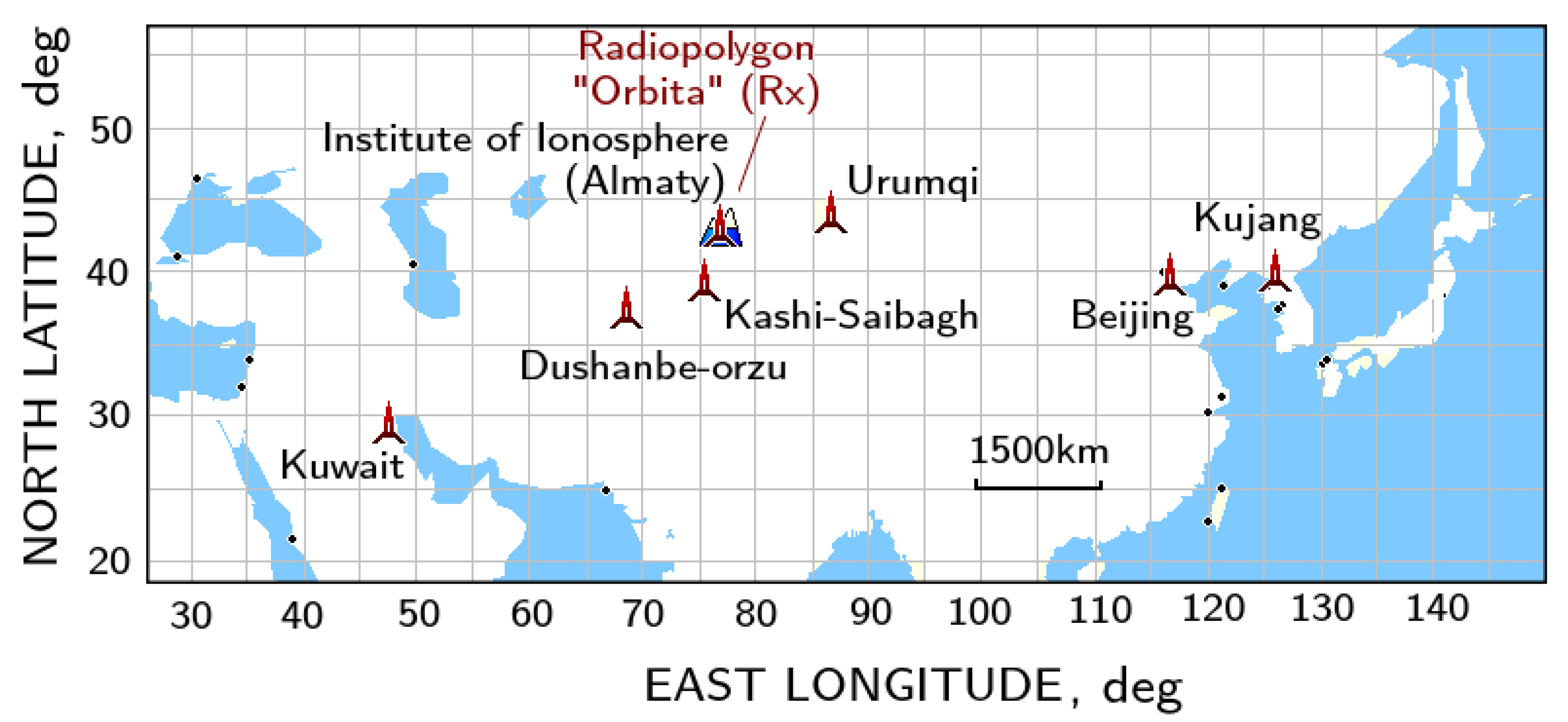

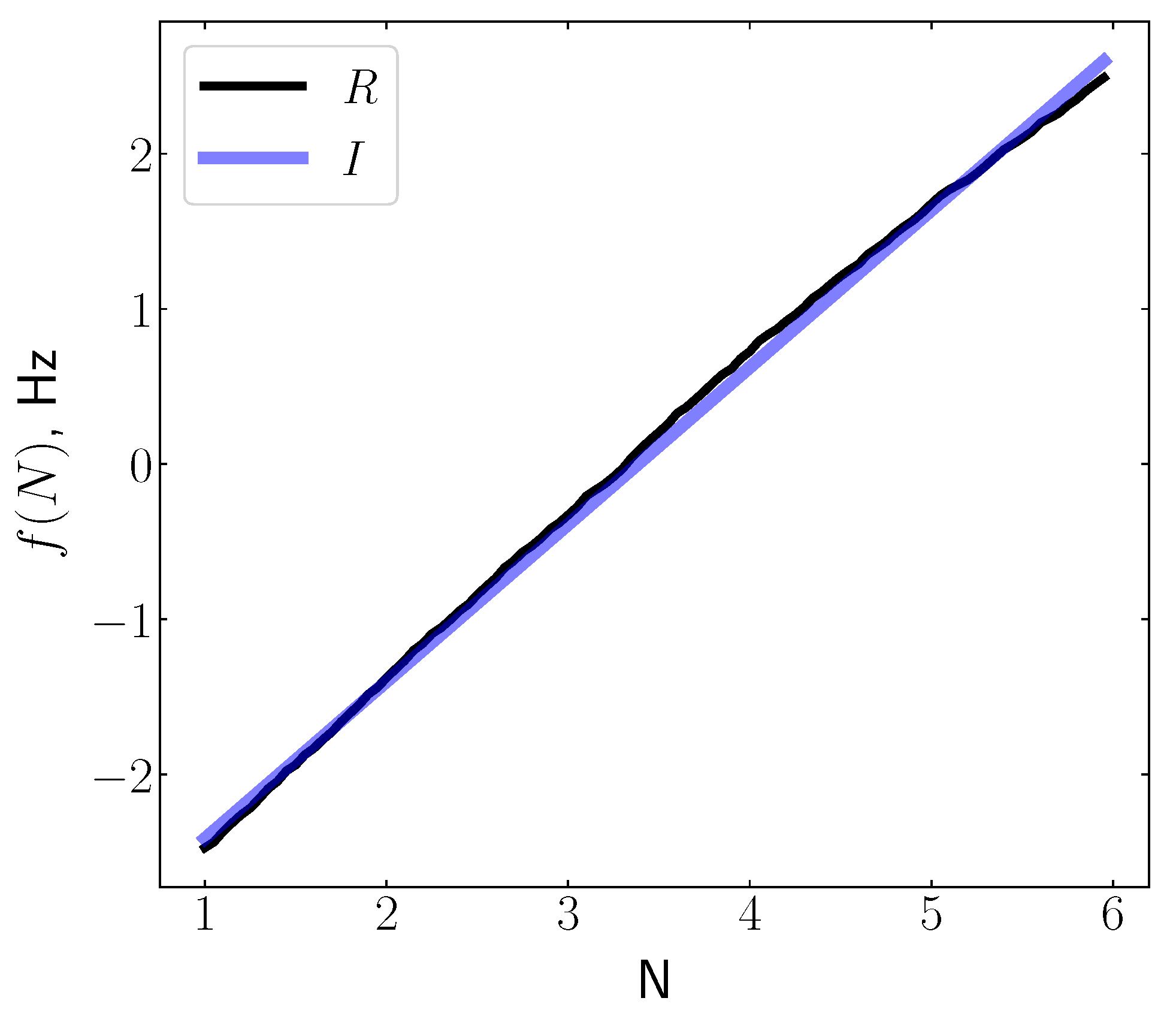
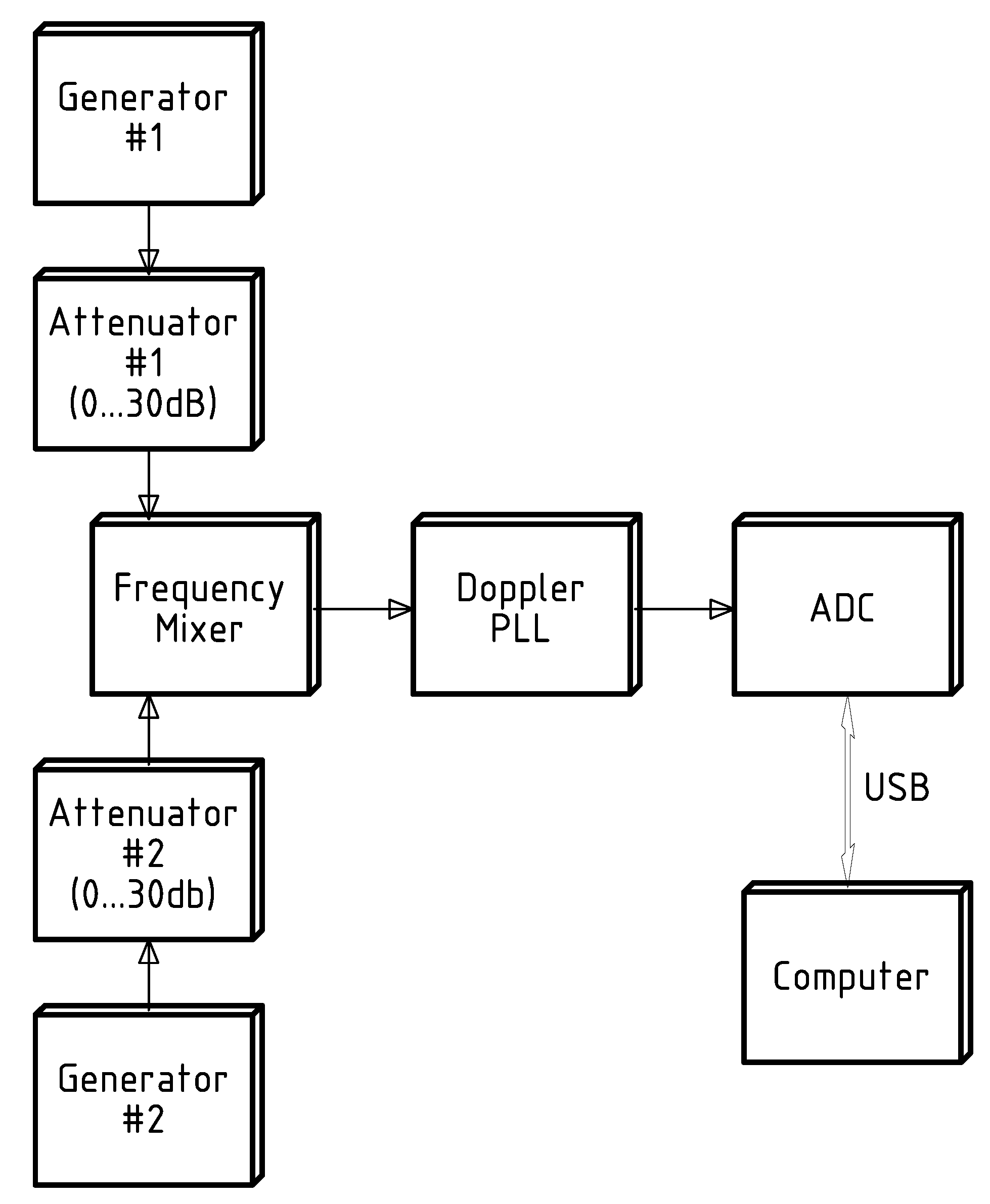
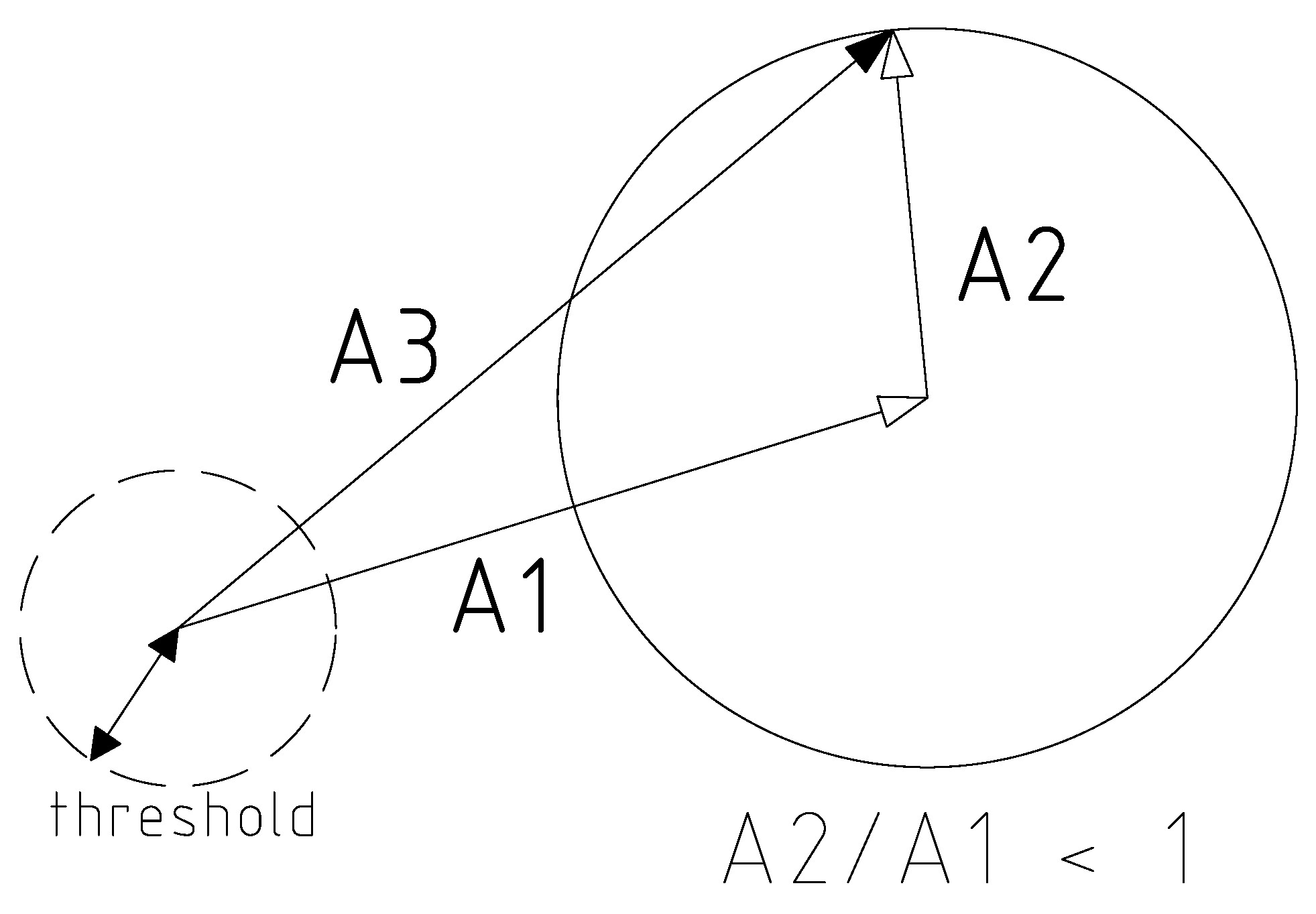

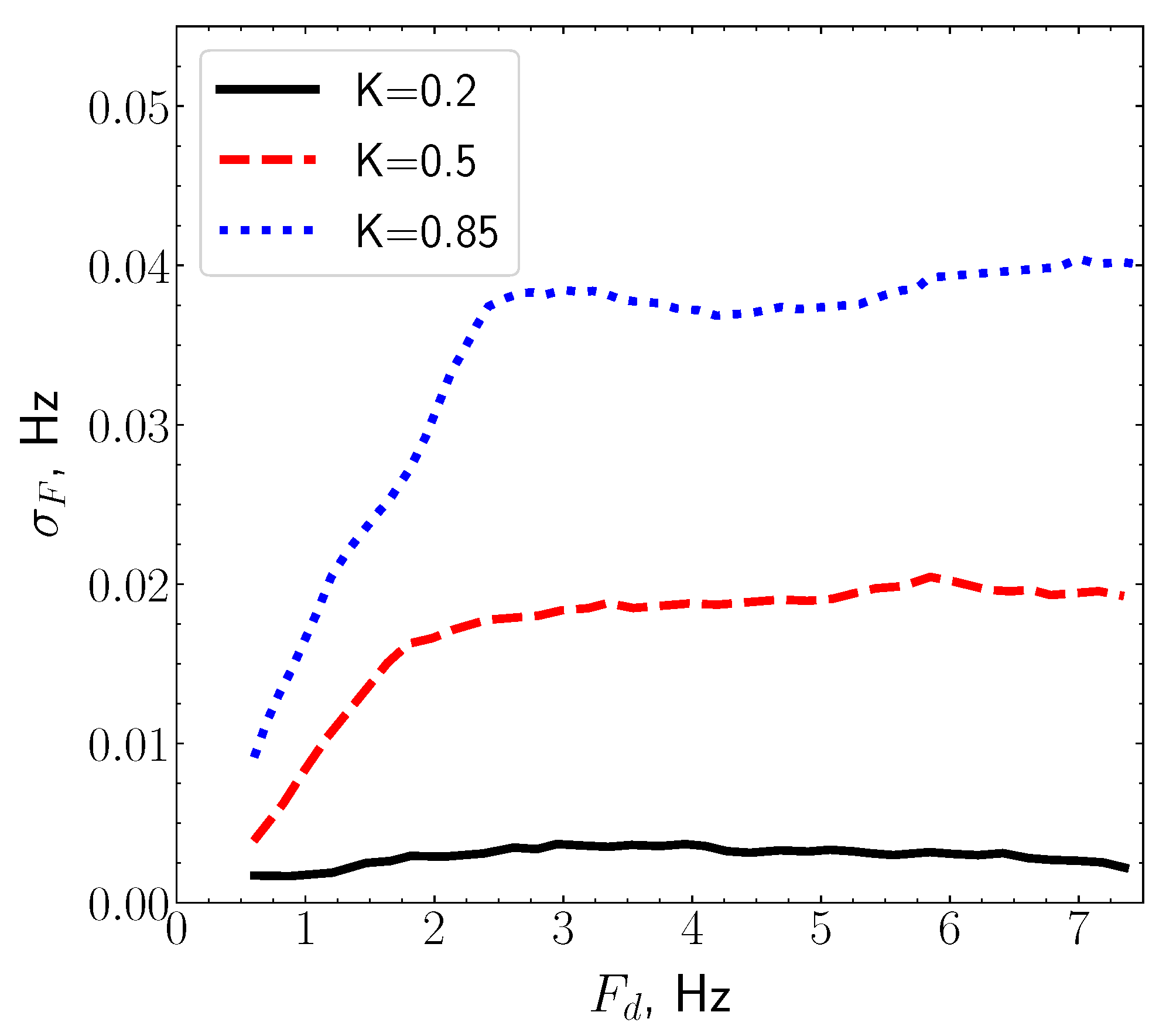

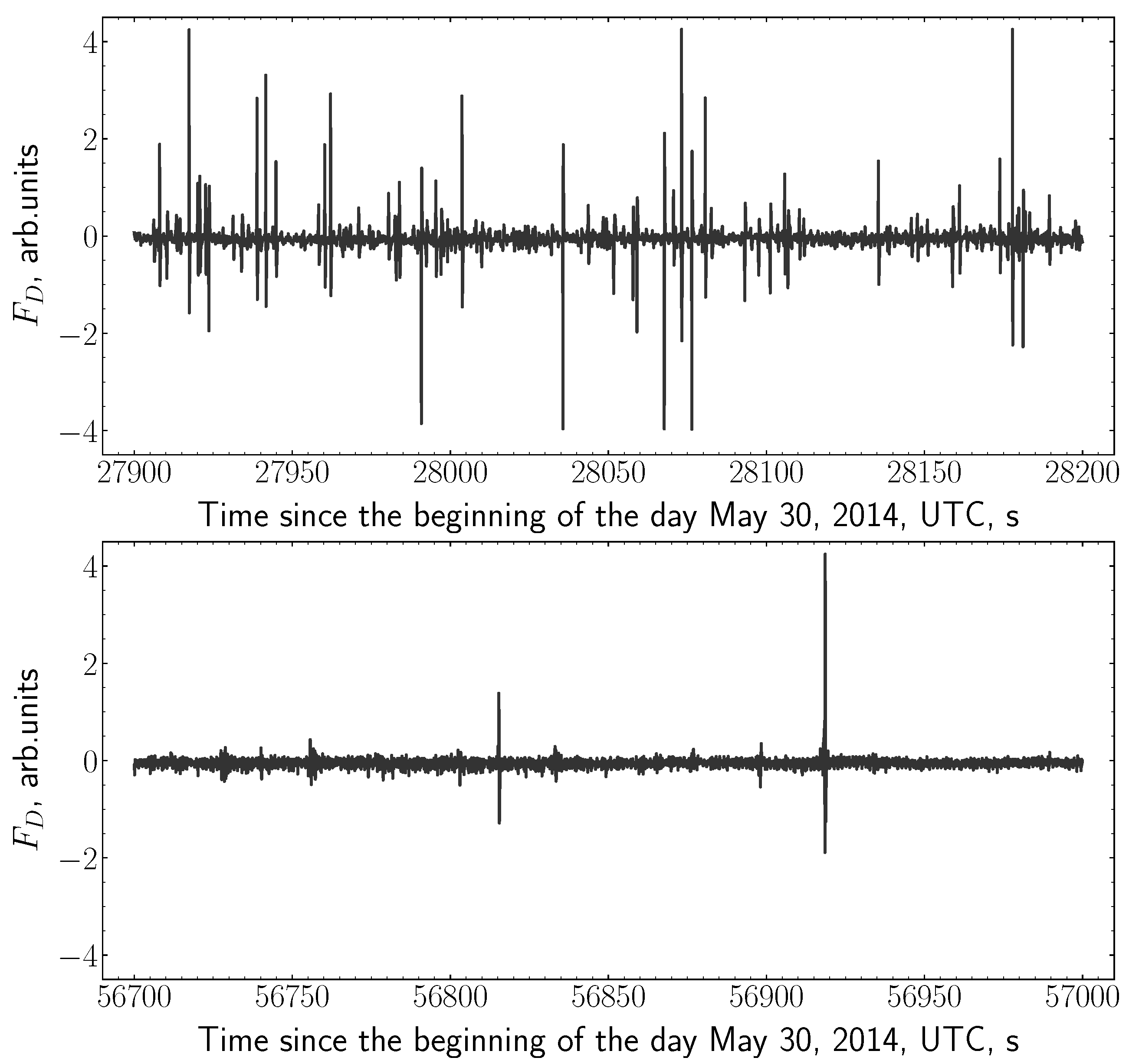
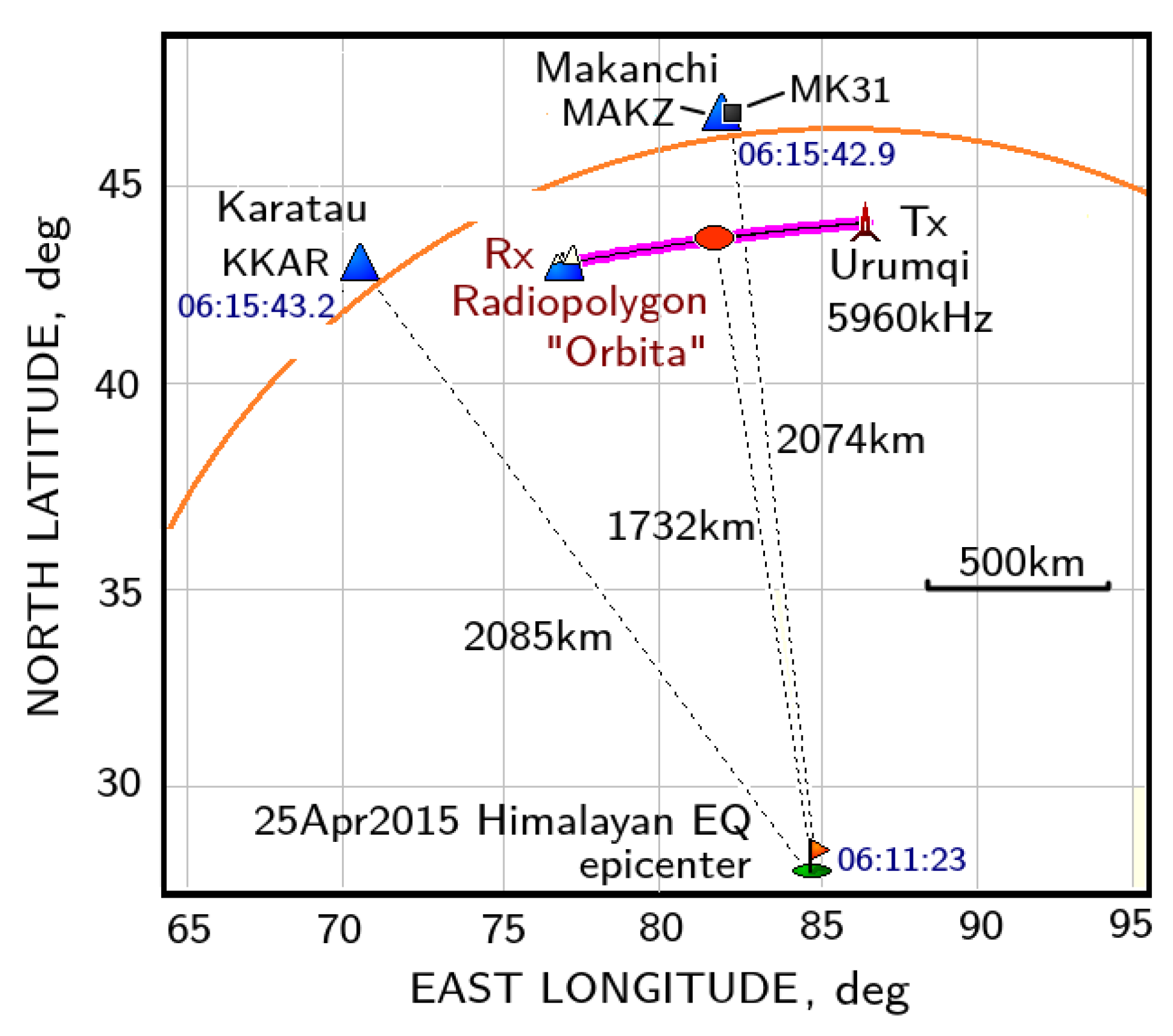
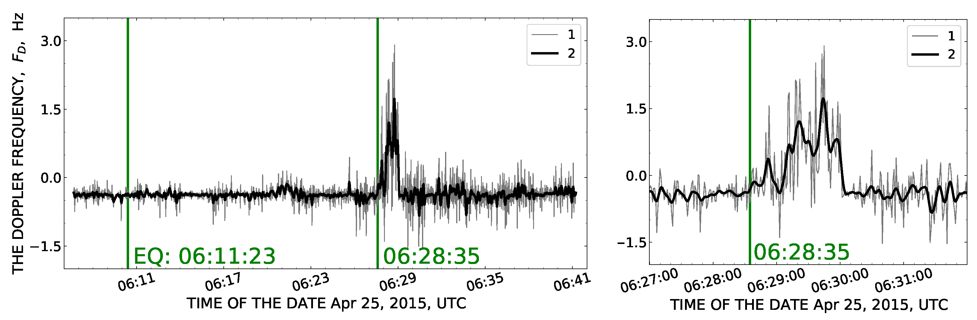
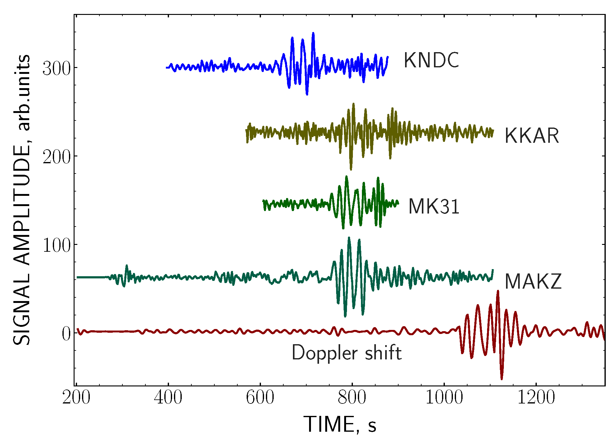
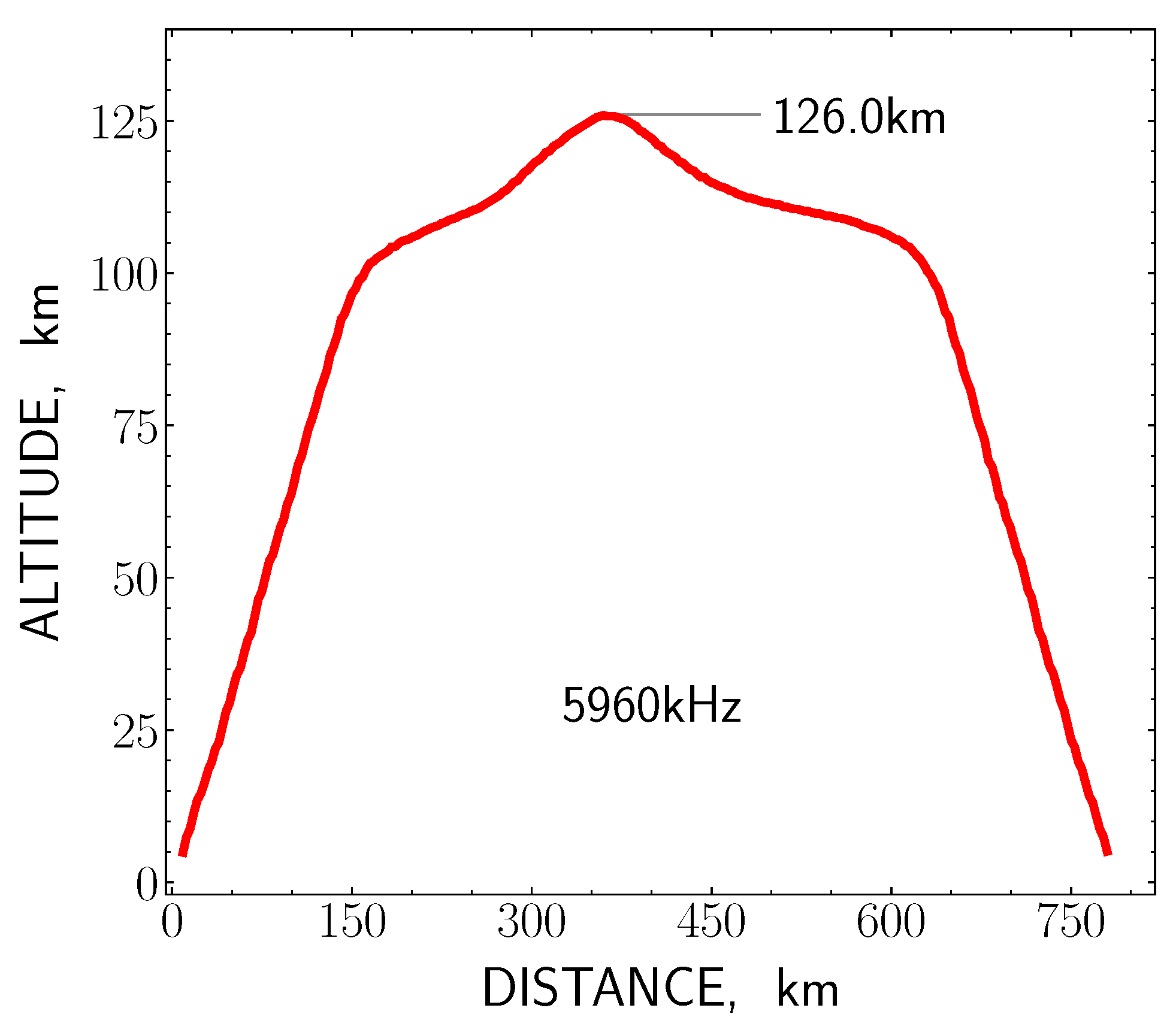
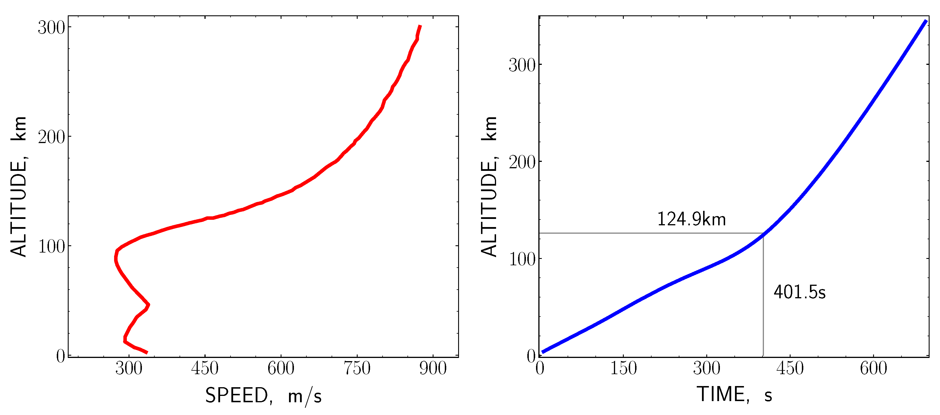
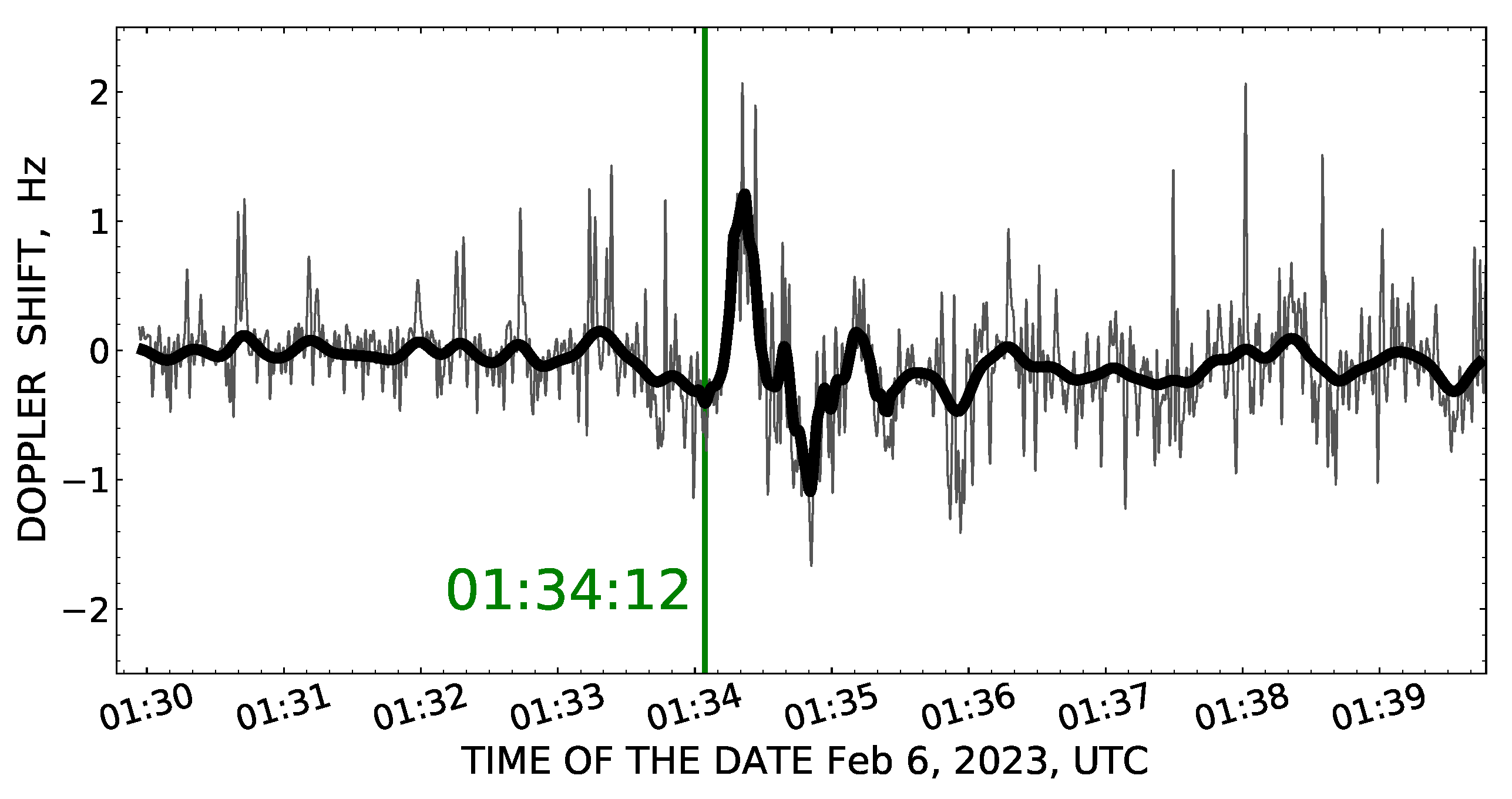
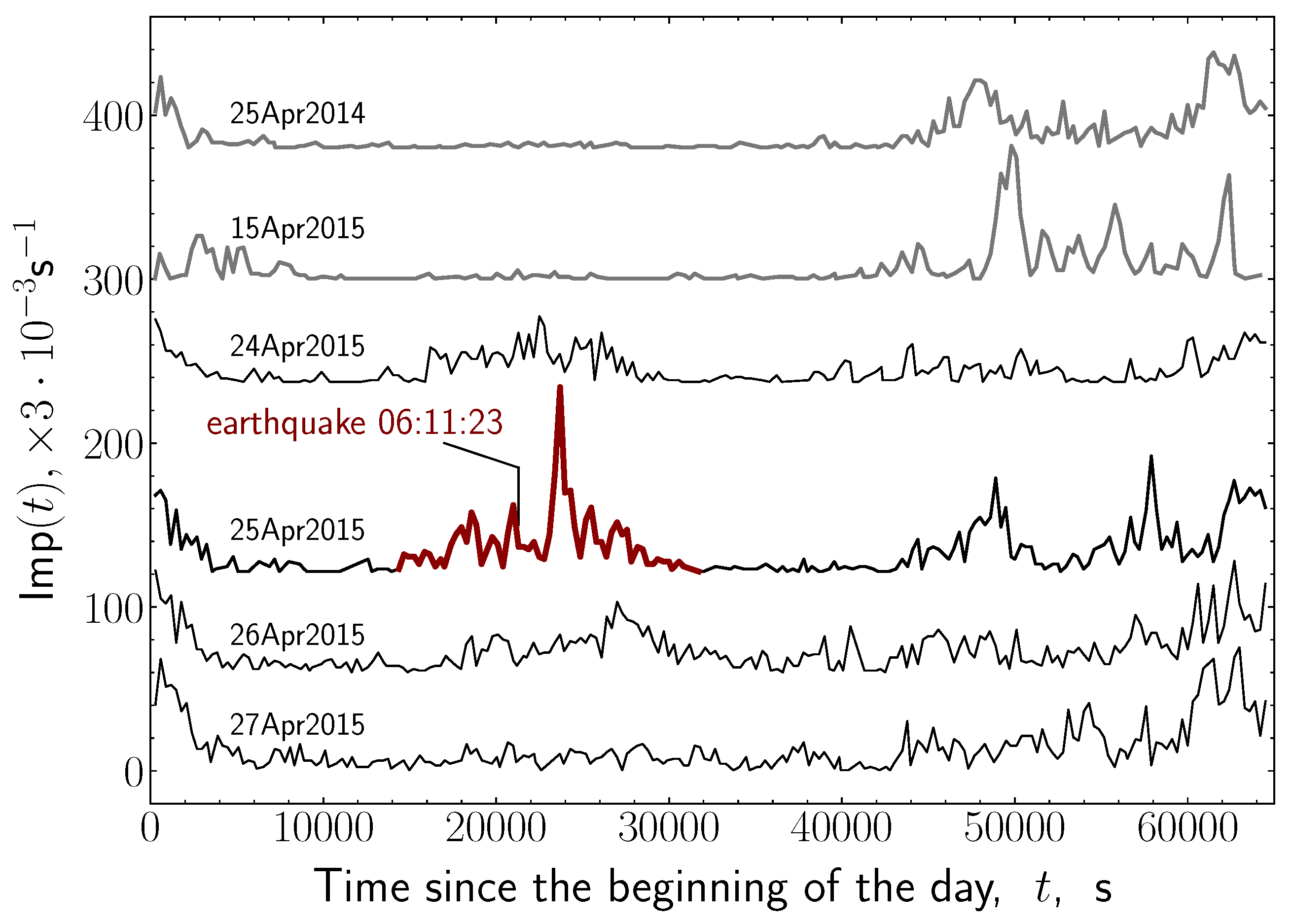

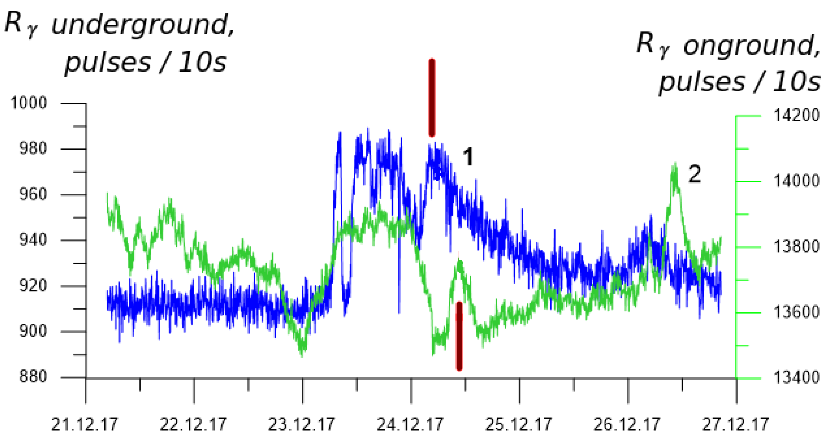
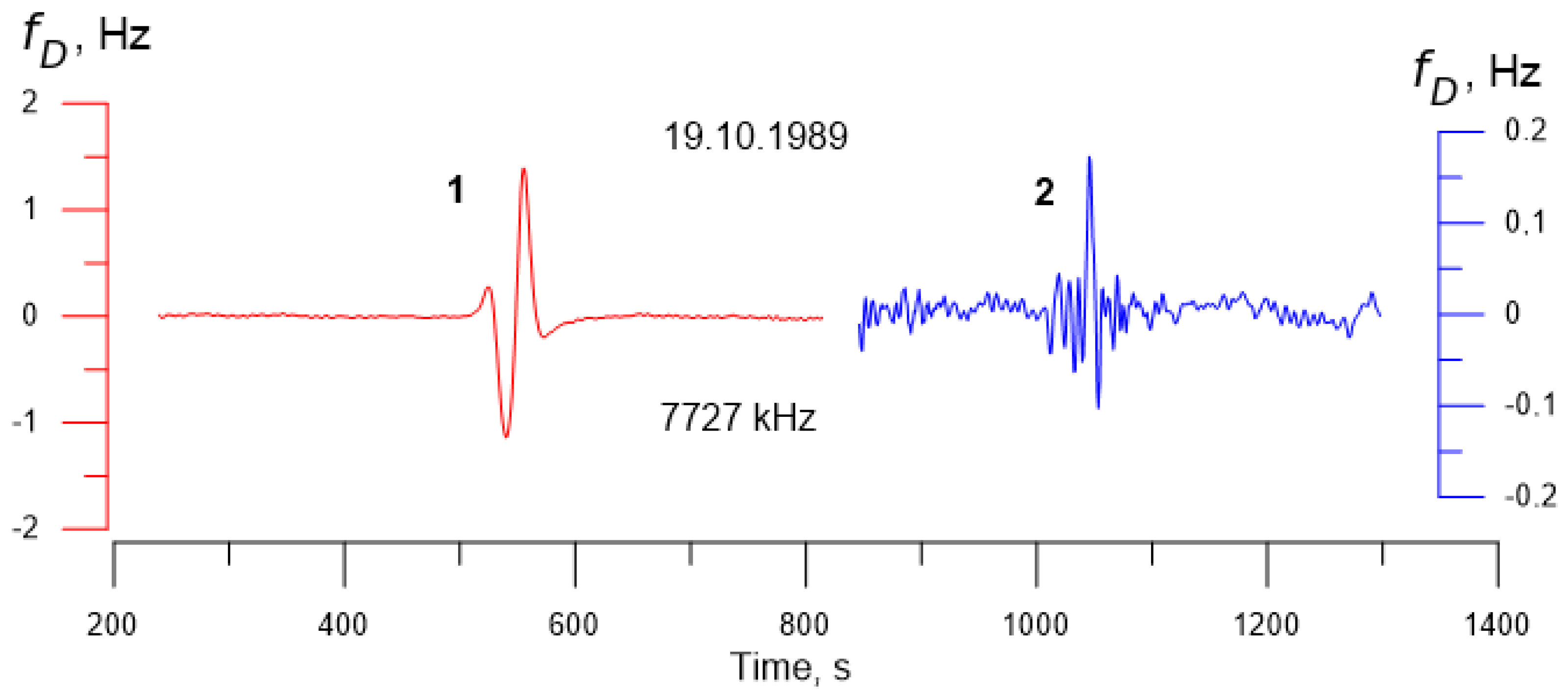
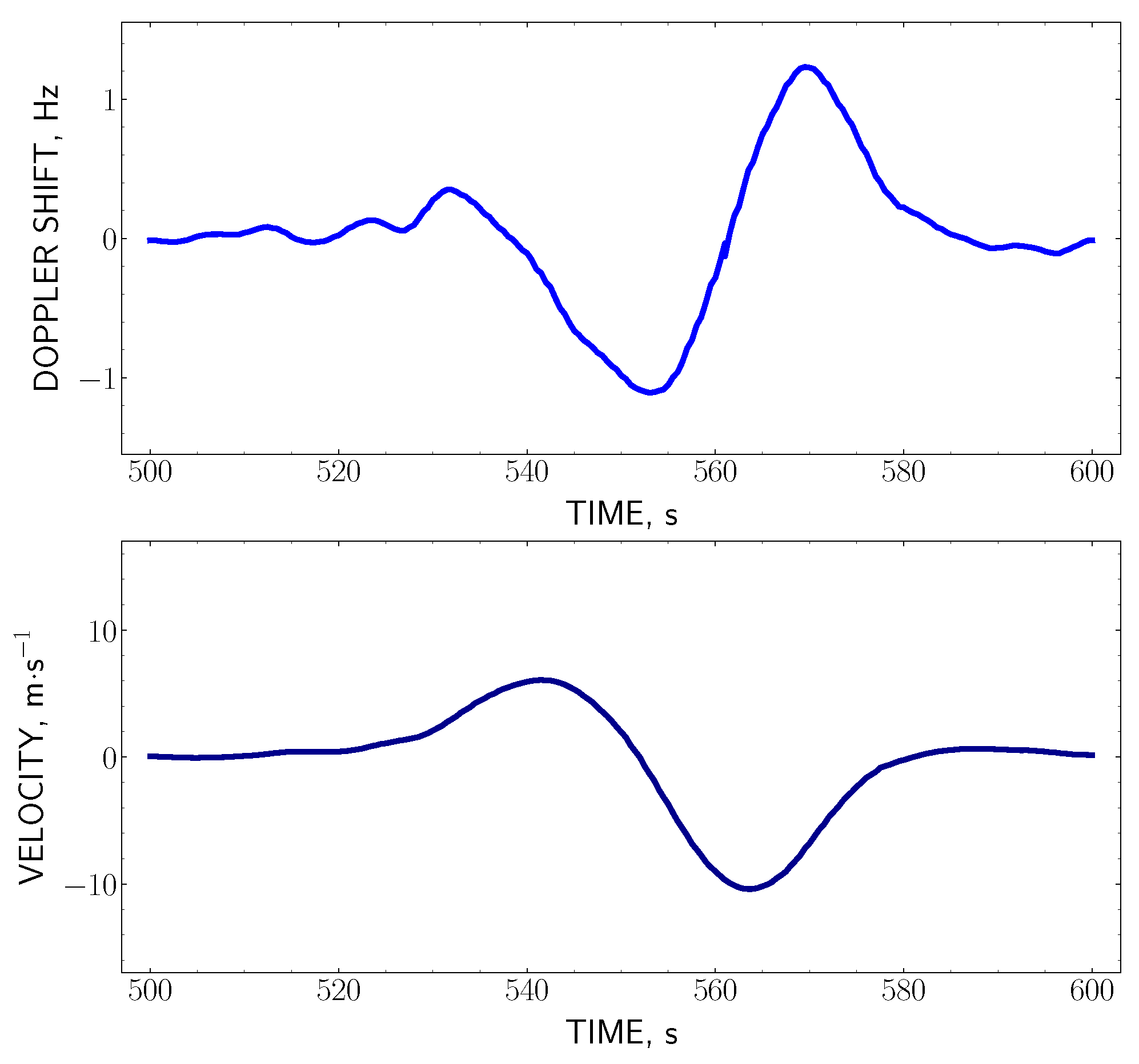

Disclaimer/Publisher’s Note: The statements, opinions and data contained in all publications are solely those of the individual author(s) and contributor(s) and not of MDPI and/or the editor(s). MDPI and/or the editor(s) disclaim responsibility for any injury to people or property resulting from any ideas, methods, instructions or products referred to in the content. |
© 2024 by the authors. Licensee MDPI, Basel, Switzerland. This article is an open access article distributed under the terms and conditions of the Creative Commons Attribution (CC BY) license (https://creativecommons.org/licenses/by/4.0/).