

Analysis of Debris Flow Protective Barriers Using the Coupled Eulerian Lagrangian Method


Abstract
:1. Introduction
2. Background
2.1. Coupled Eulerian Lagrangian Method (CEL)
- The Lagrangian step, including the following source term:
- 2.
- The Eulerian step, containing the following convective term:
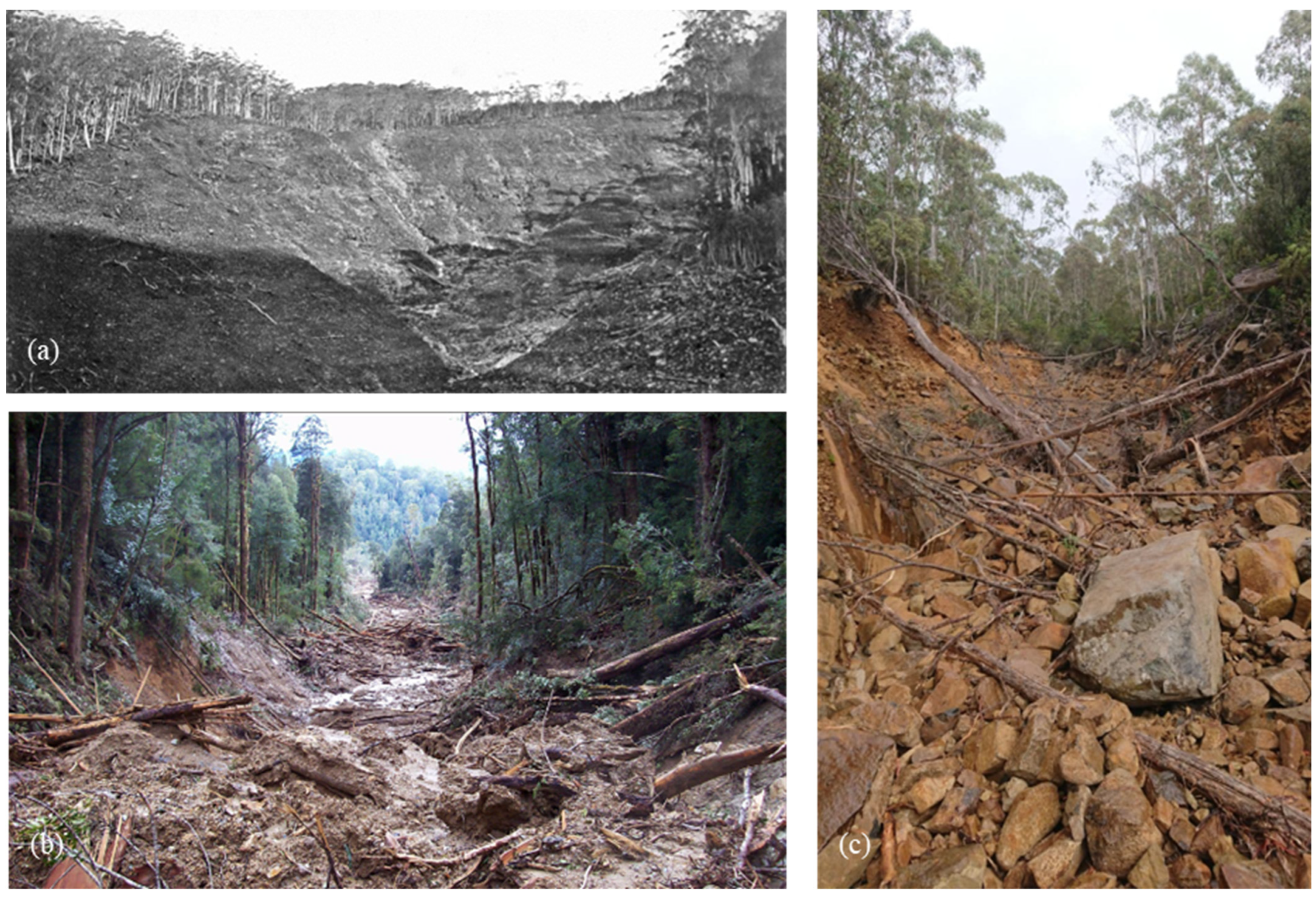
2.2. Debris Flow Hazard in Tasmania, Australia
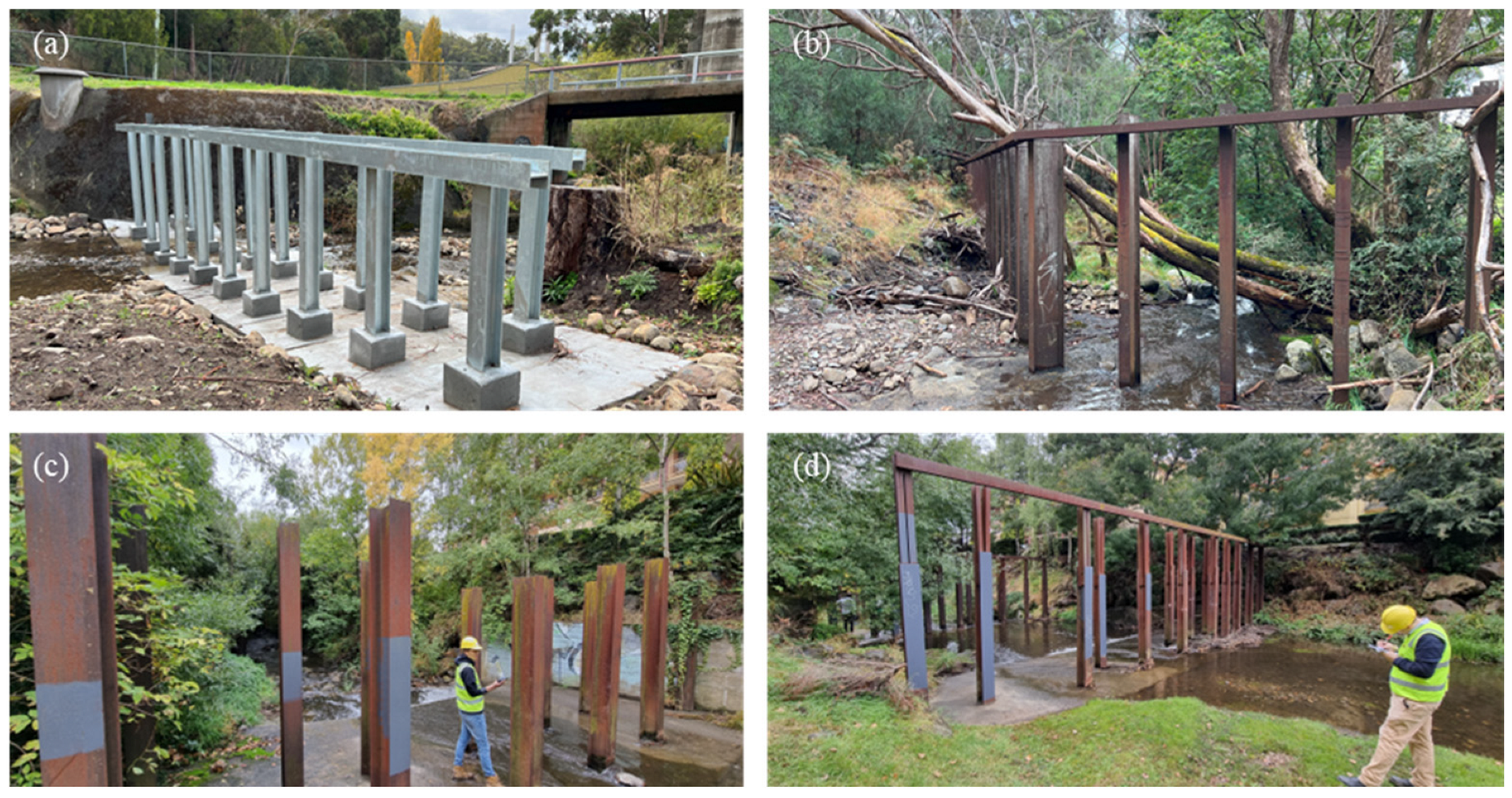
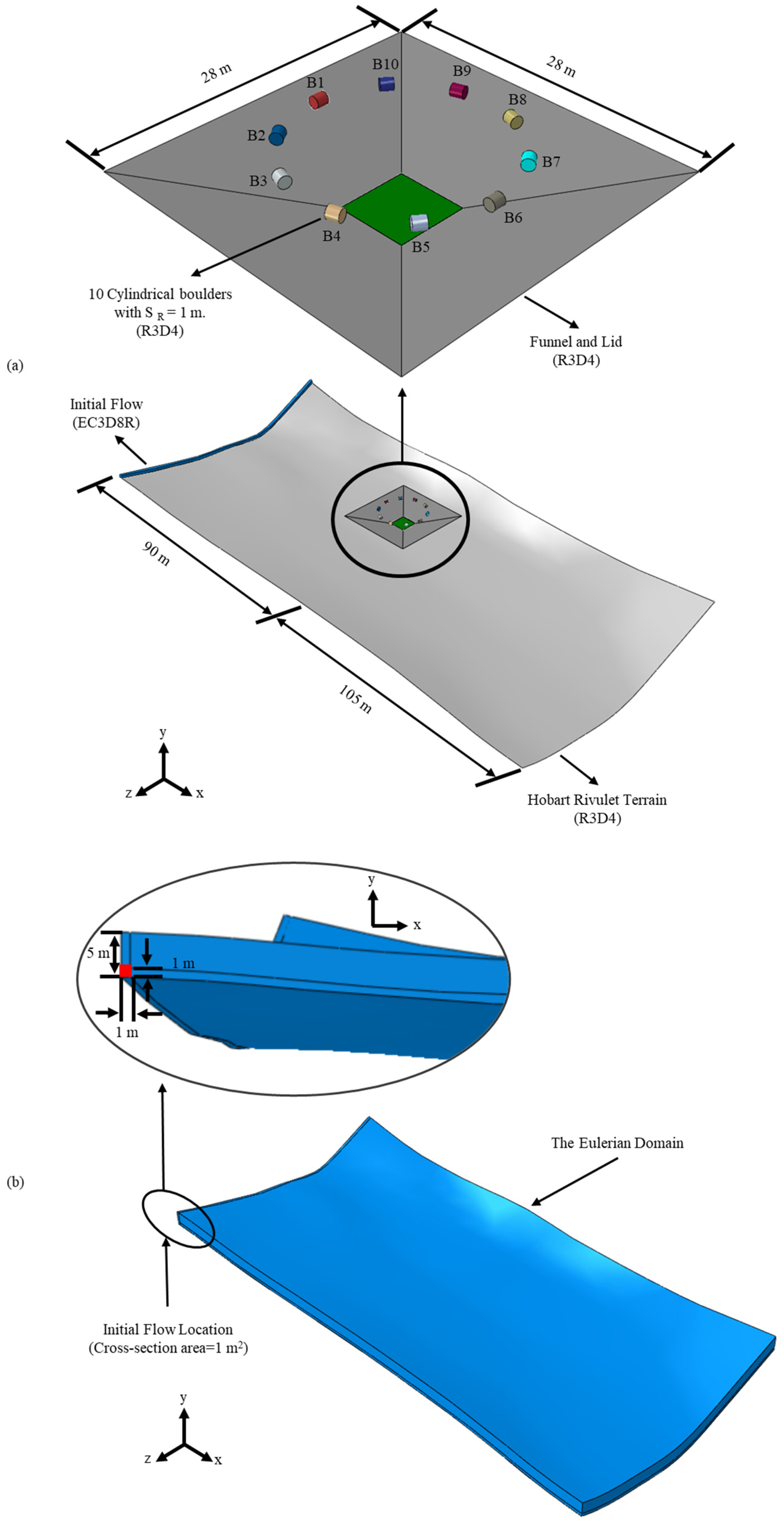
2.3. Study Area and Current Protective Structures
2.4. Rheological Model of Debris Flow
3. Performance Assessment and Comparison
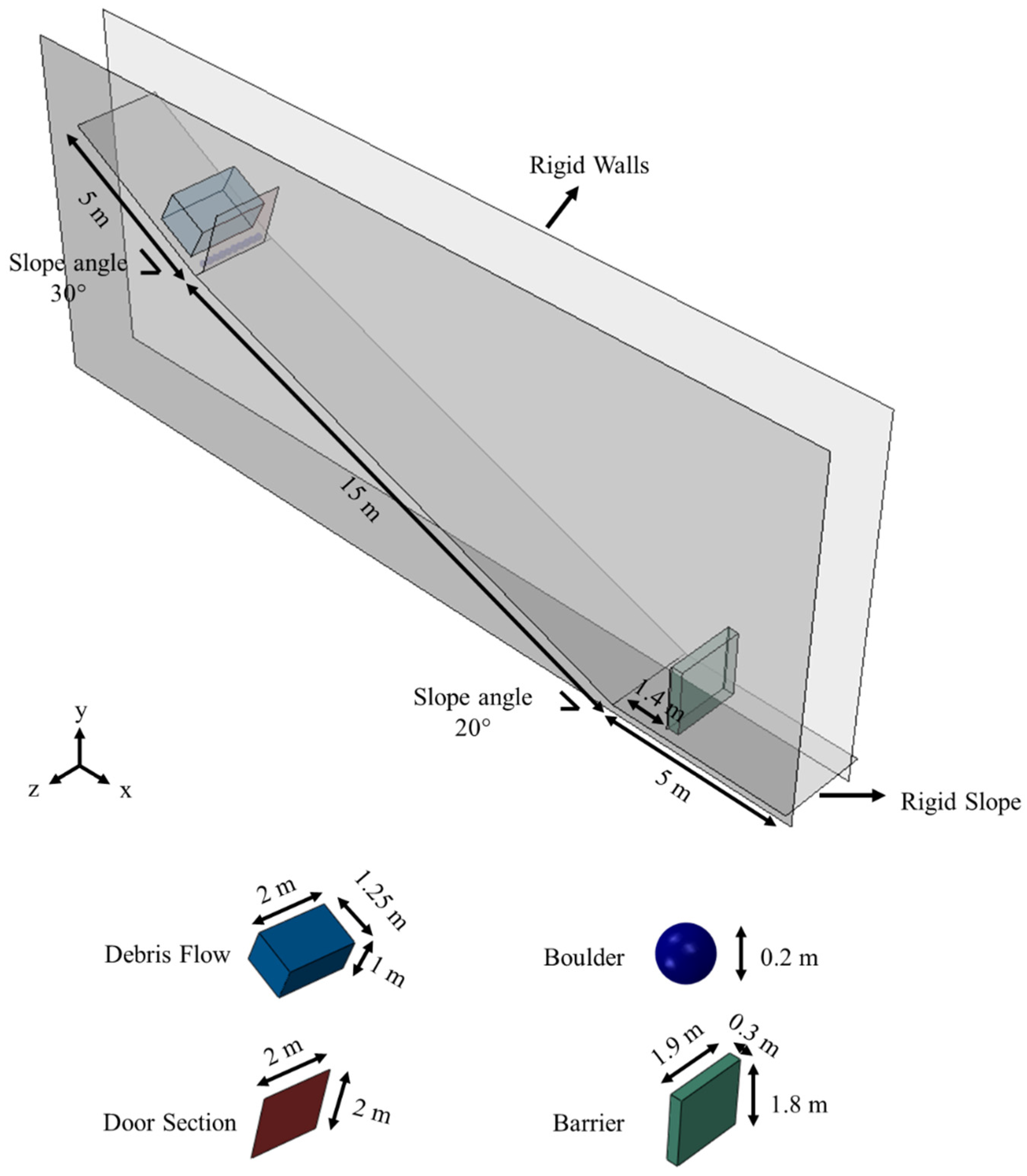
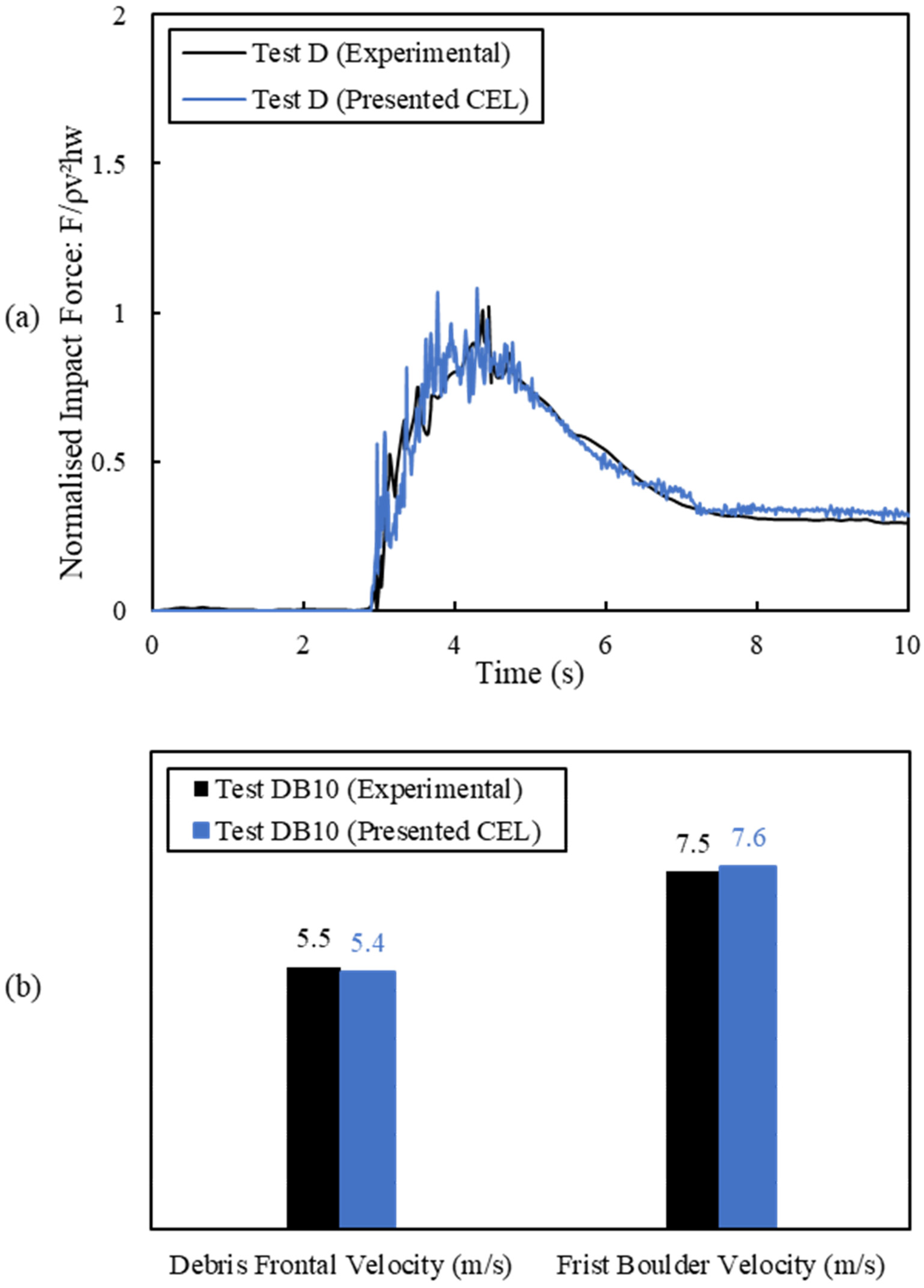
3.1. Model Validation
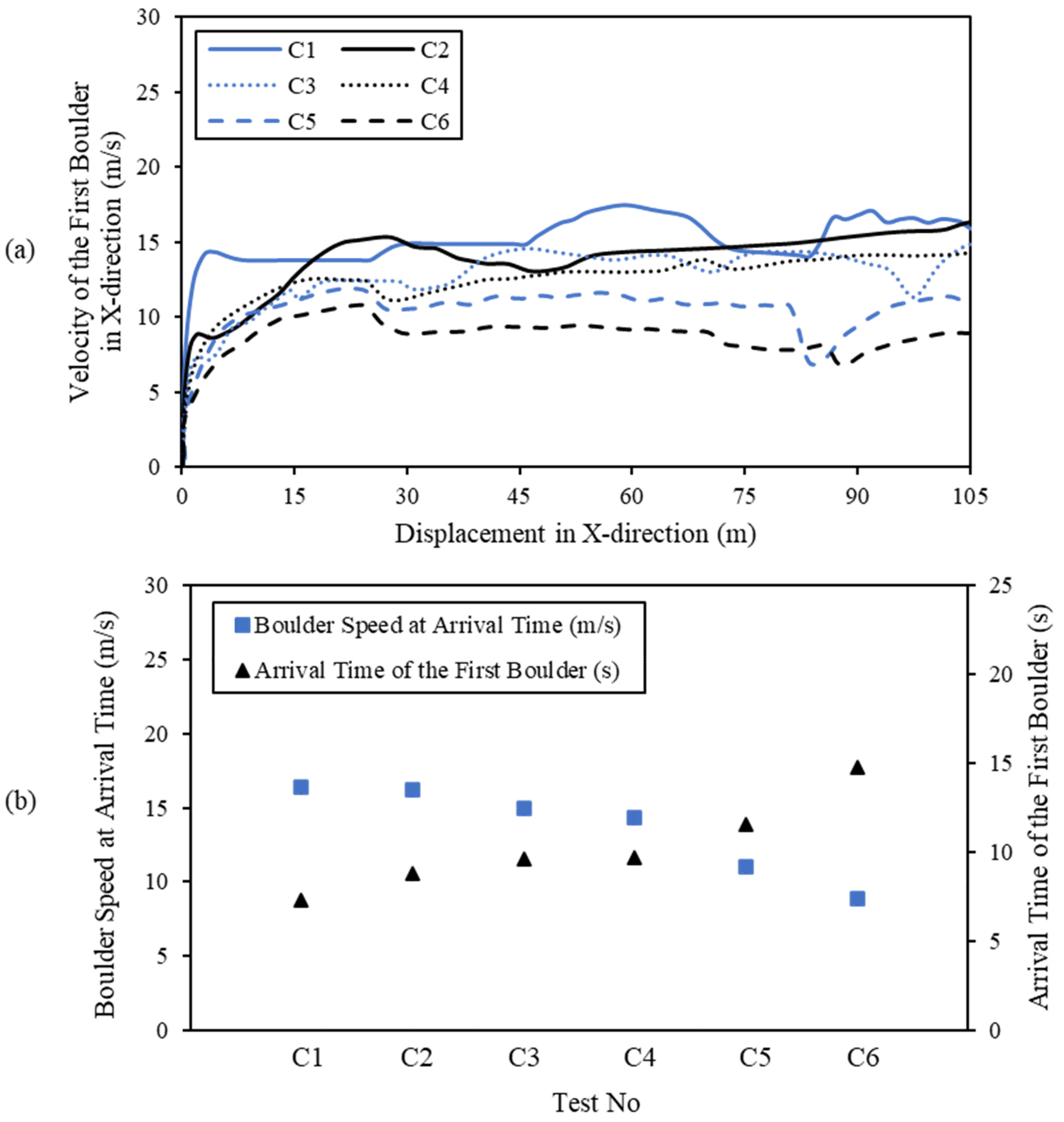
3.2. Estimation of Boulder Velocity on Hobart Rivulet Terrain
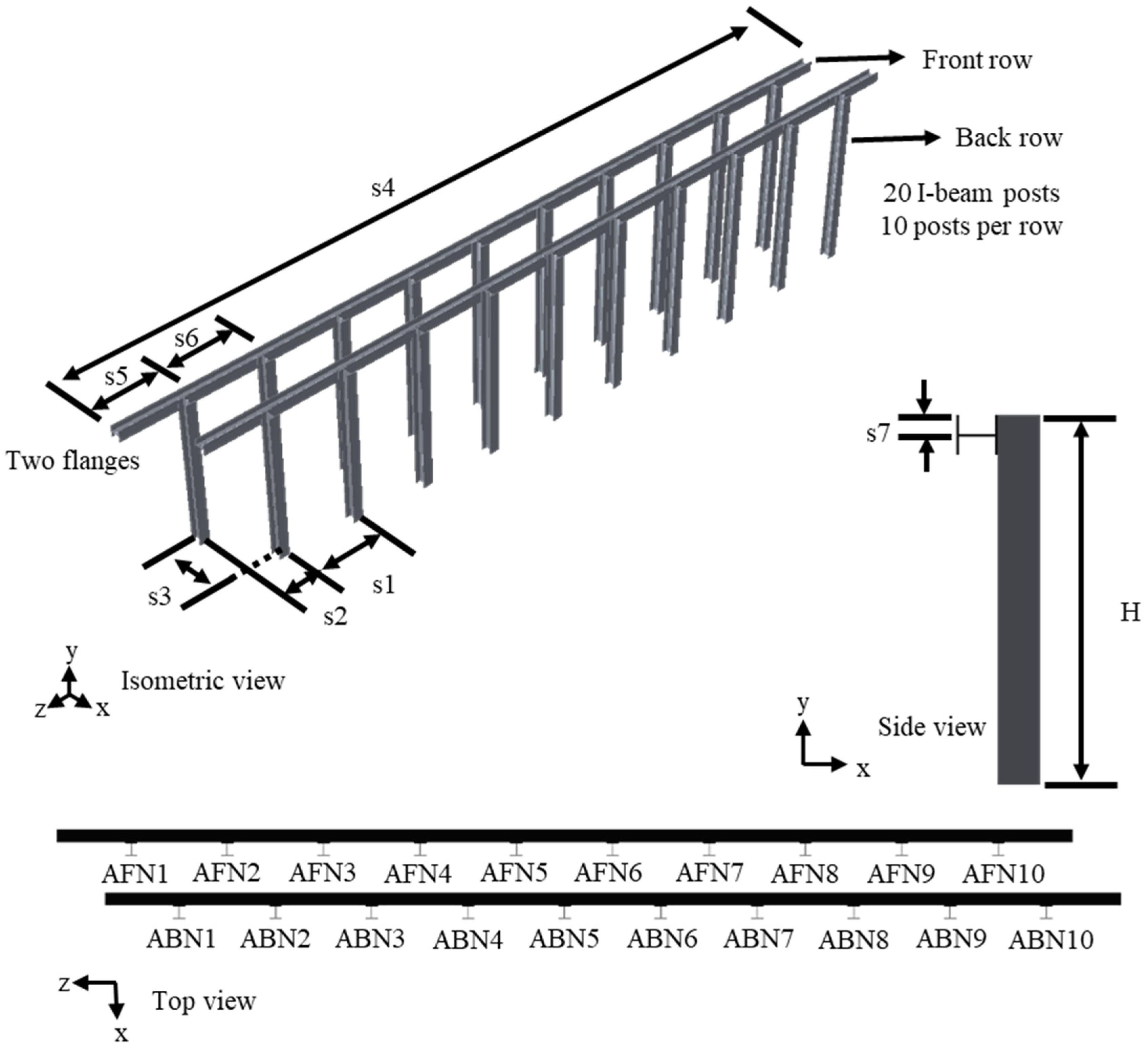
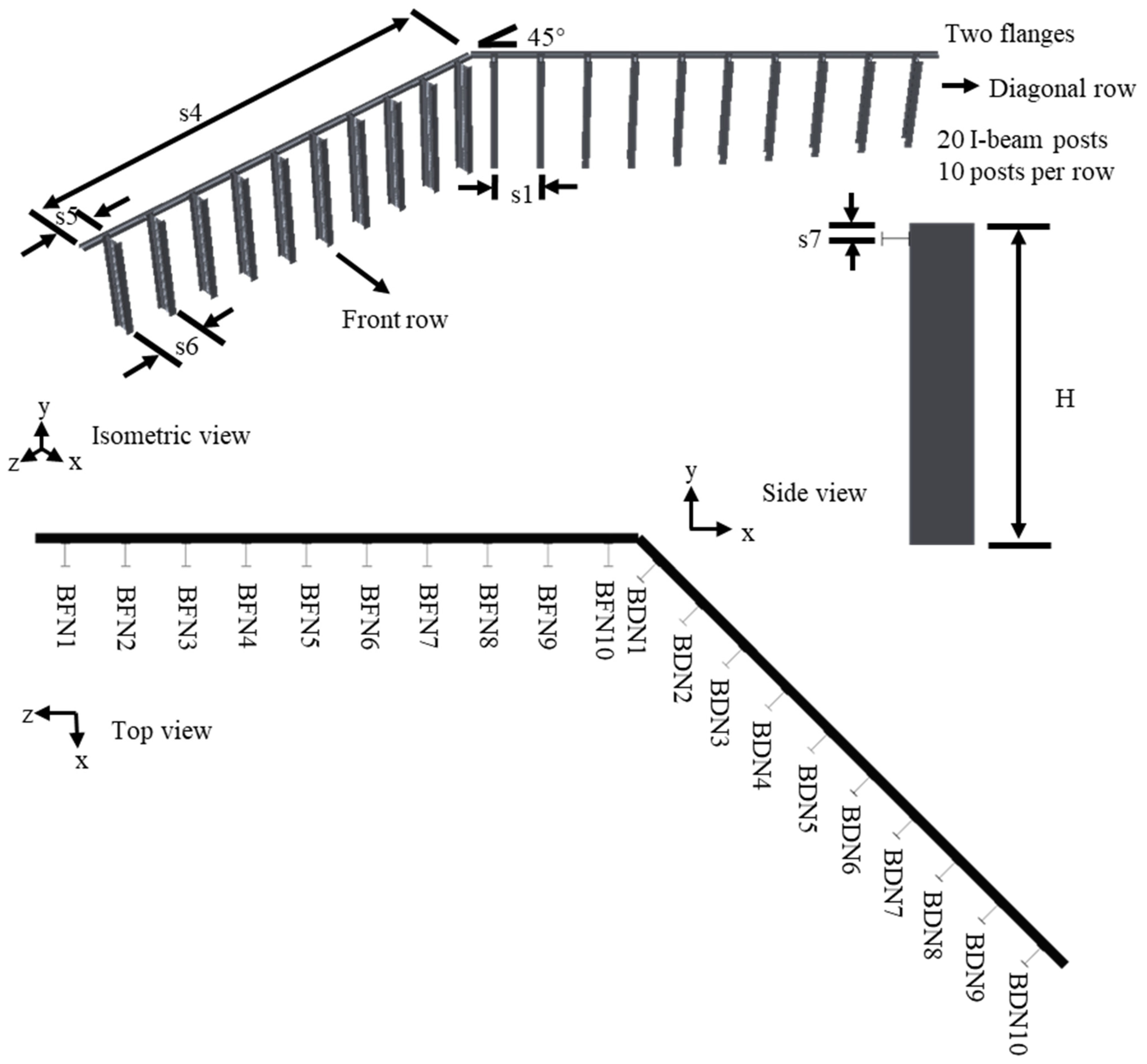
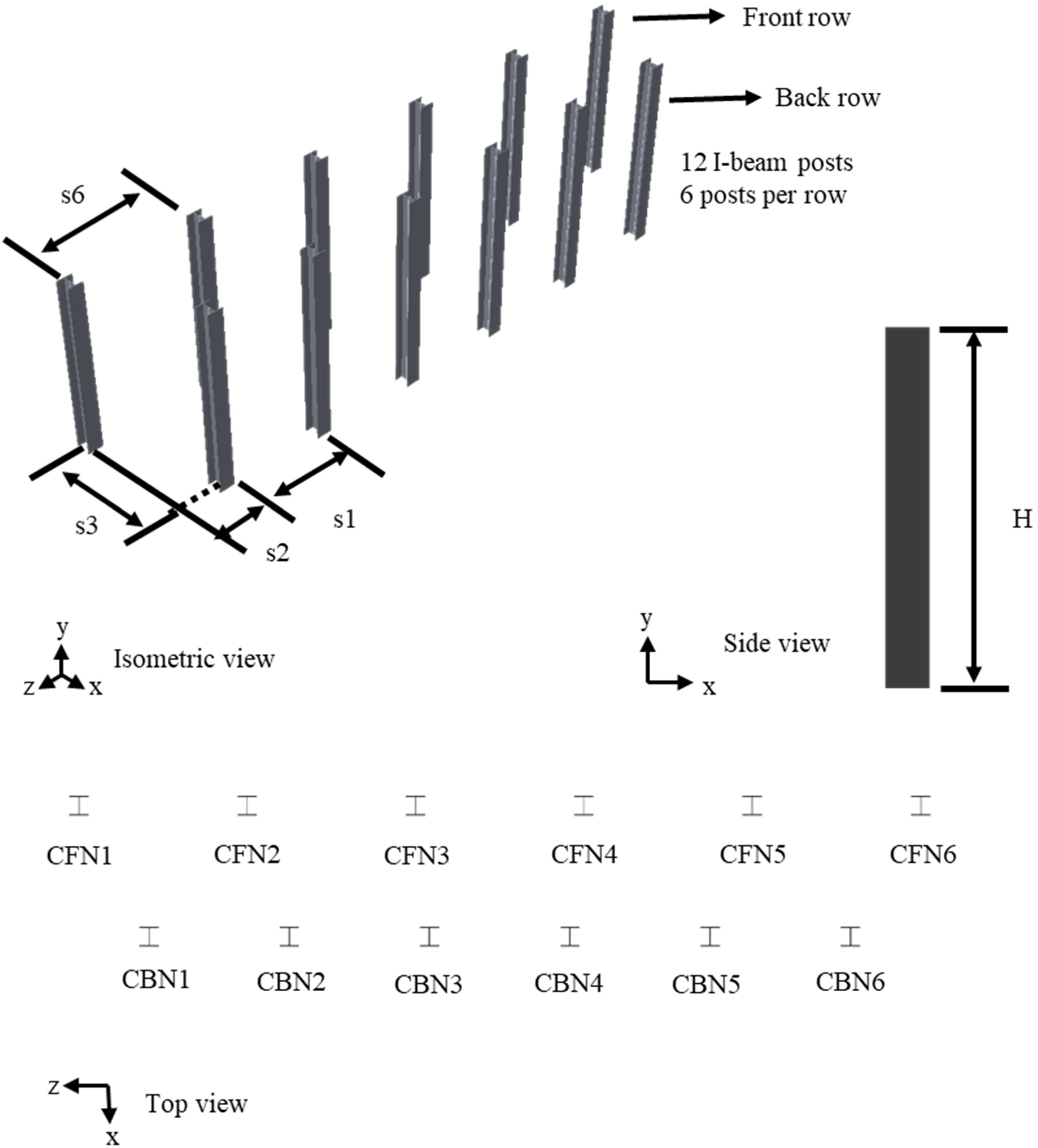
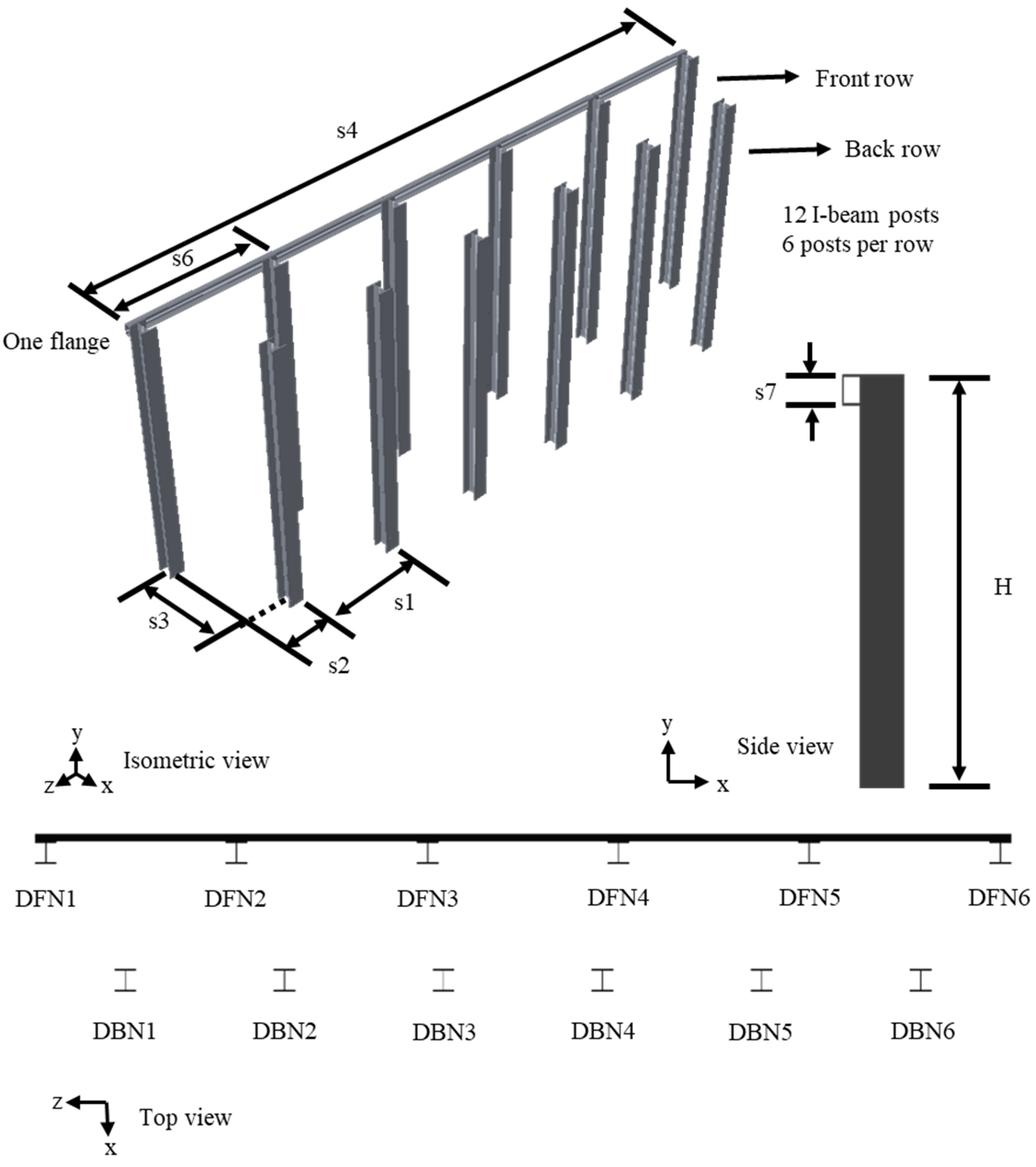
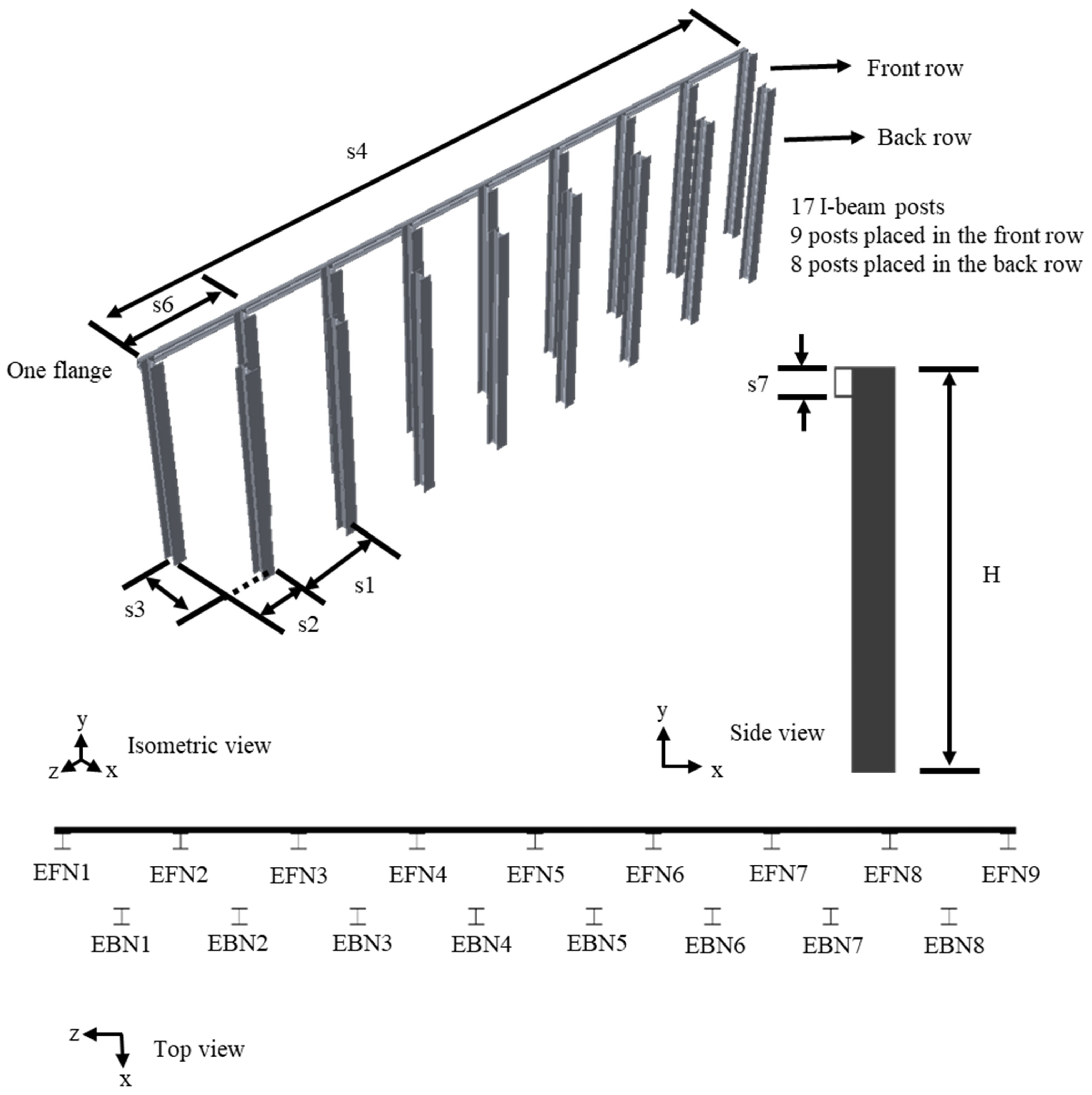
3.3. Dimensions of I-Beam Post Barriers
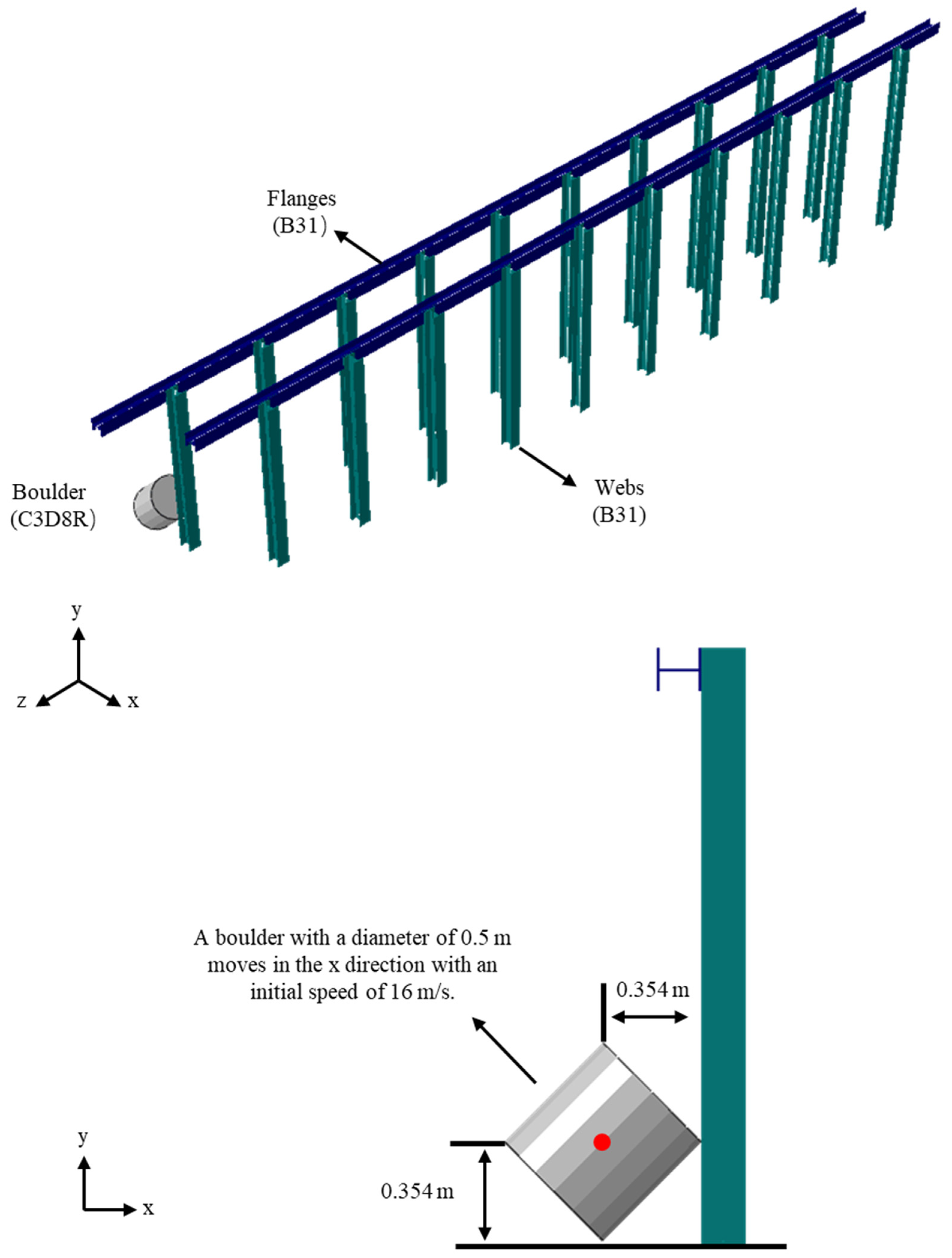
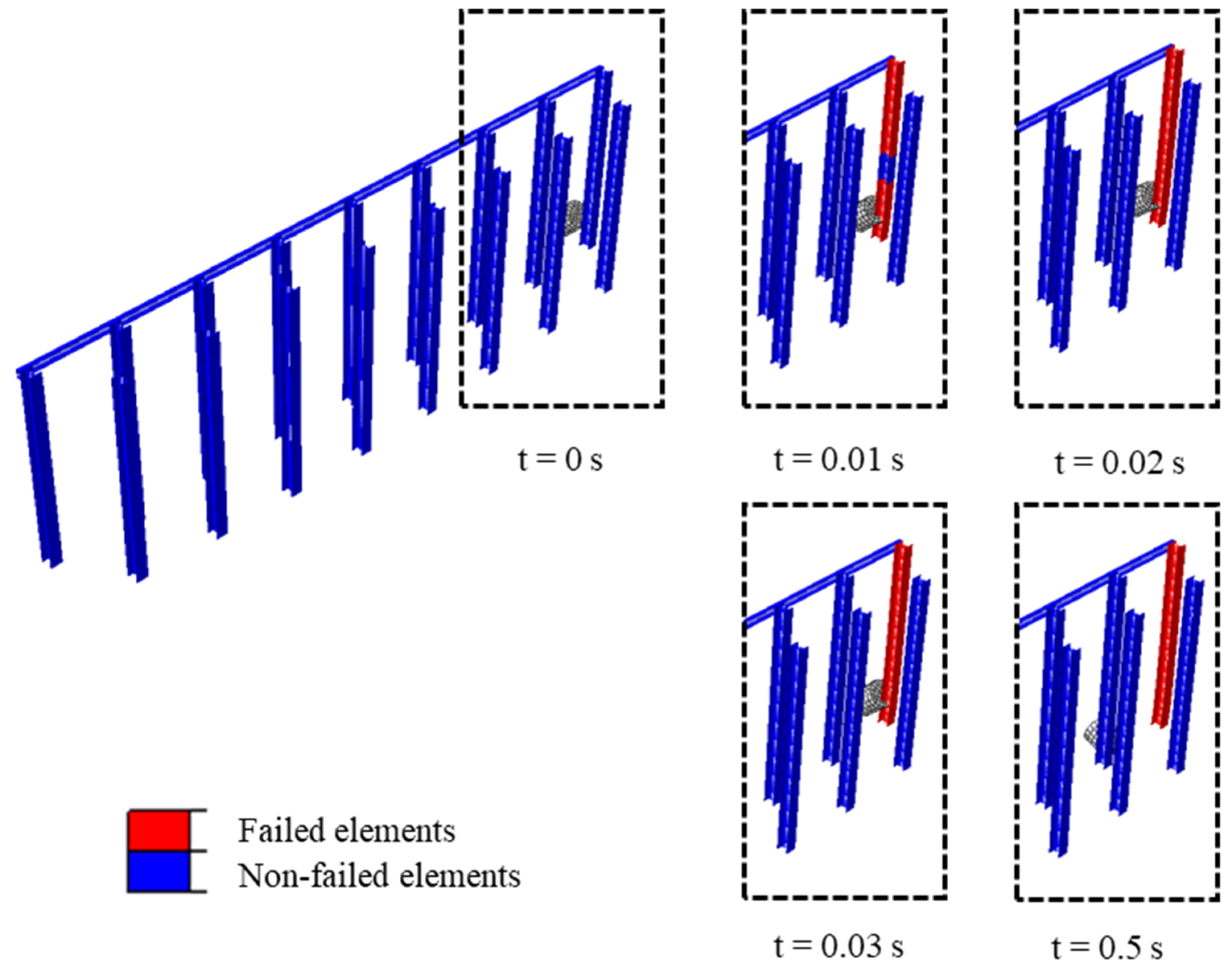
3.4. Modelling of Boulder–Barrier Interactions
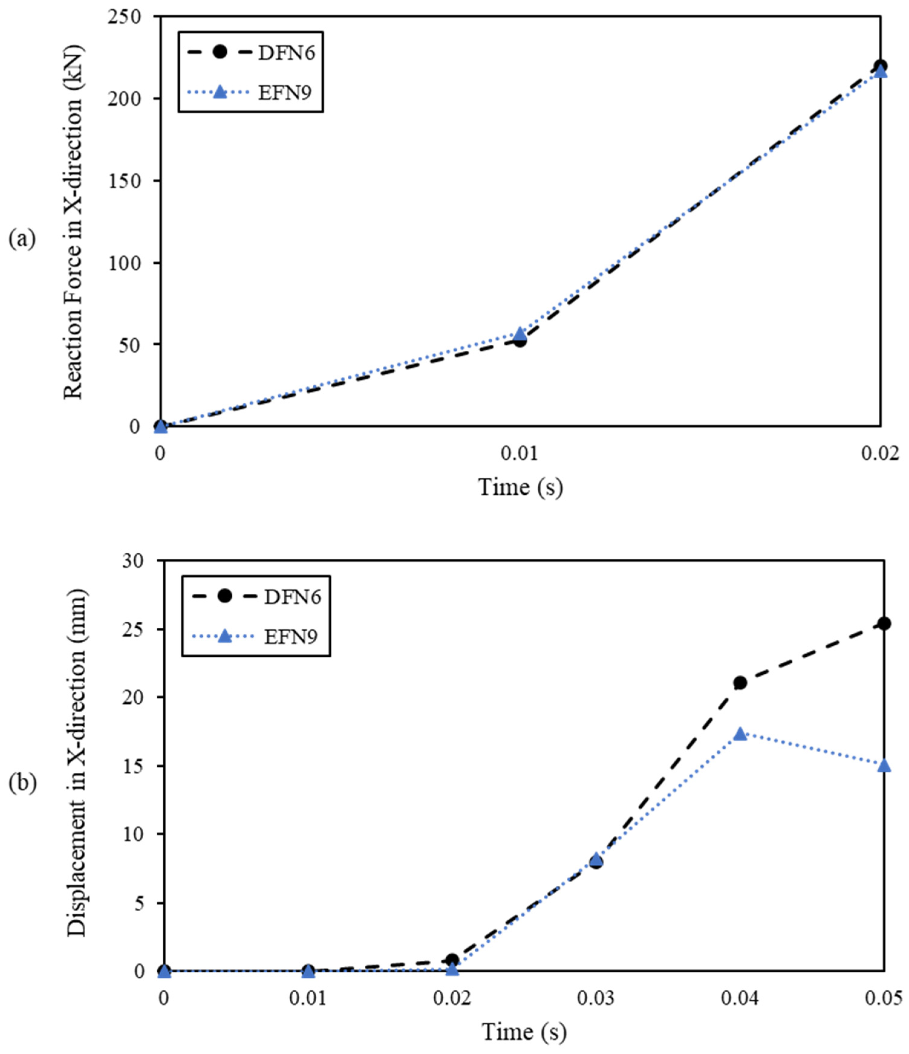
3.5. Results and Comparison
4. Conclusions
- To validate the CEL model, the Bingham model was employed to simulate experimental debris flow tests as conducted by Ng et al. [44]. The simulation results, encompassing impact force and velocities of the debris front and first arrival boulder, exhibited a good agreement with the experimental data. These findings affirm that the CEL model can effectively provide precise estimations of boulder velocities post impact with debris flow;
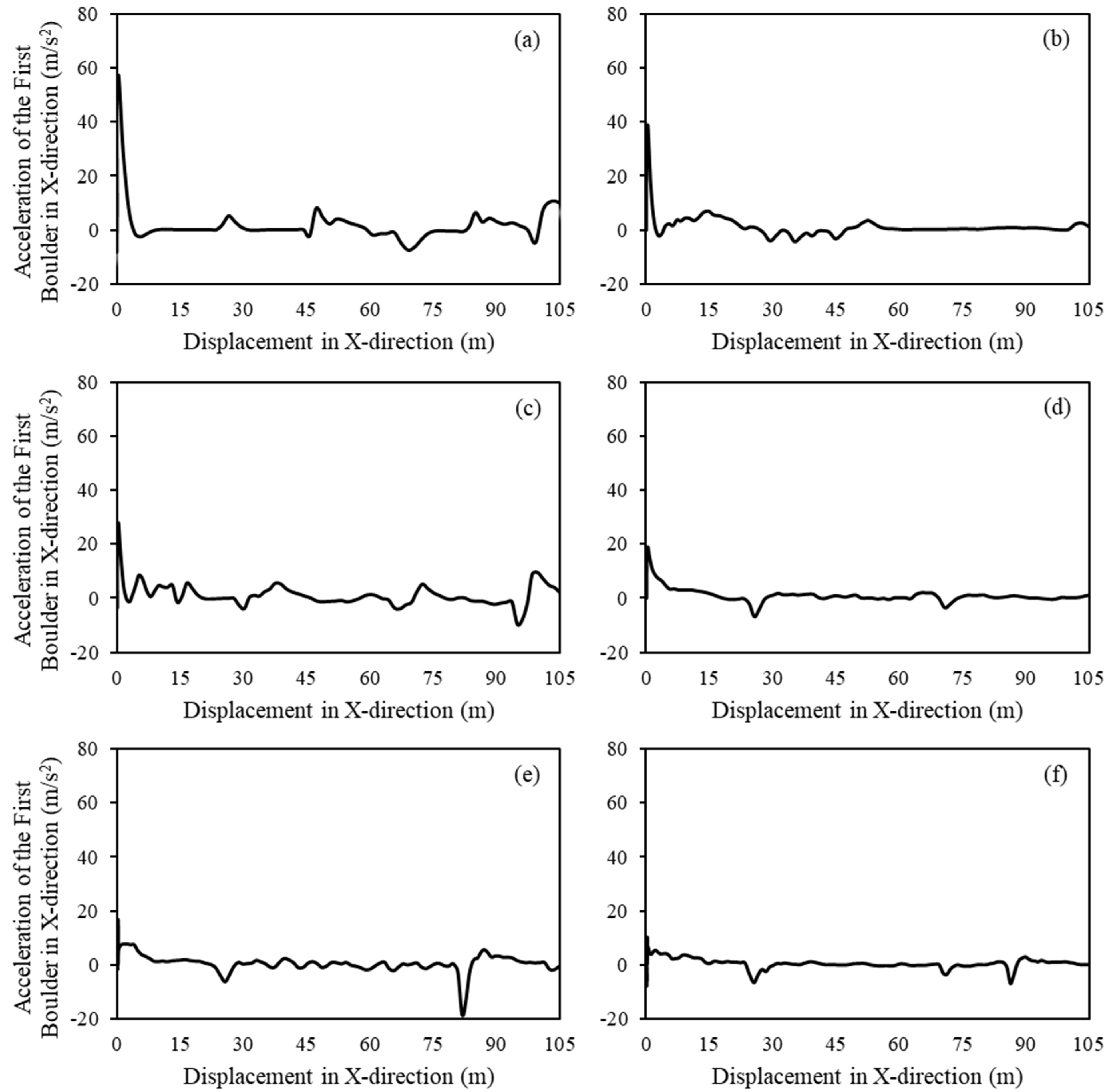
- Analysis of simulation tests conducted with various boulder sizes on the Hobart Rivulet terrain revealed that larger boulders exhibit slower velocities and longer travel durations compared to smaller boulders due to their greater mass. Fluctuations in velocity patterns across various boulder sizes highlight the influence of irregular terrain surfaces on boulder dynamics. Notably, the initial contact between the flow and the boulder significantly affects velocity and travel time, with smaller boulders experiencing higher accelerations upon impact;
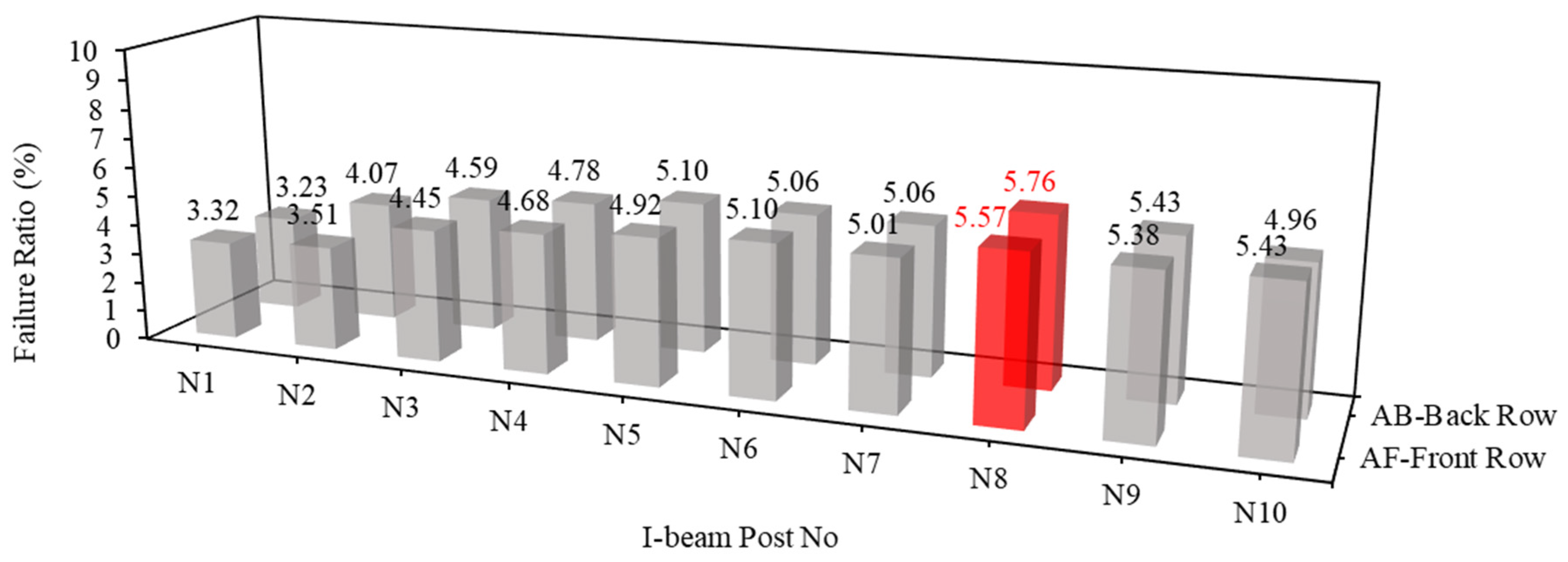
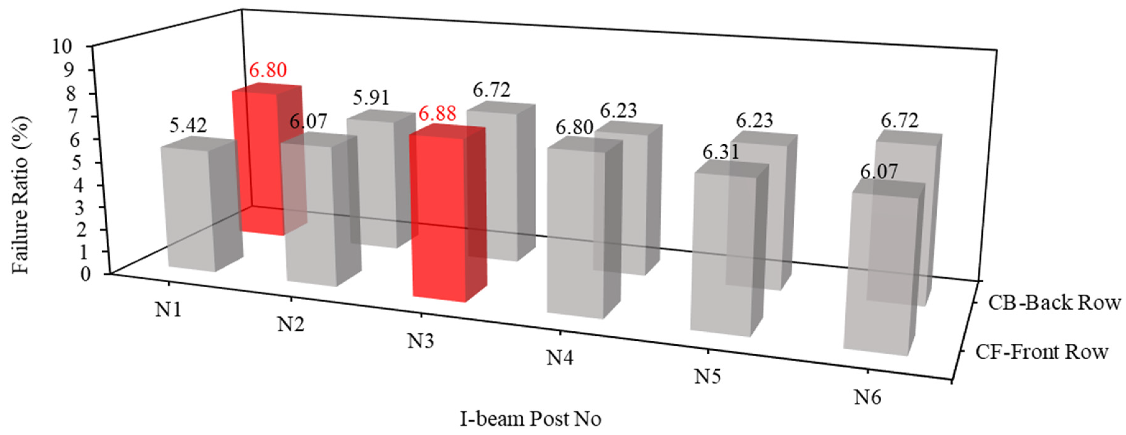
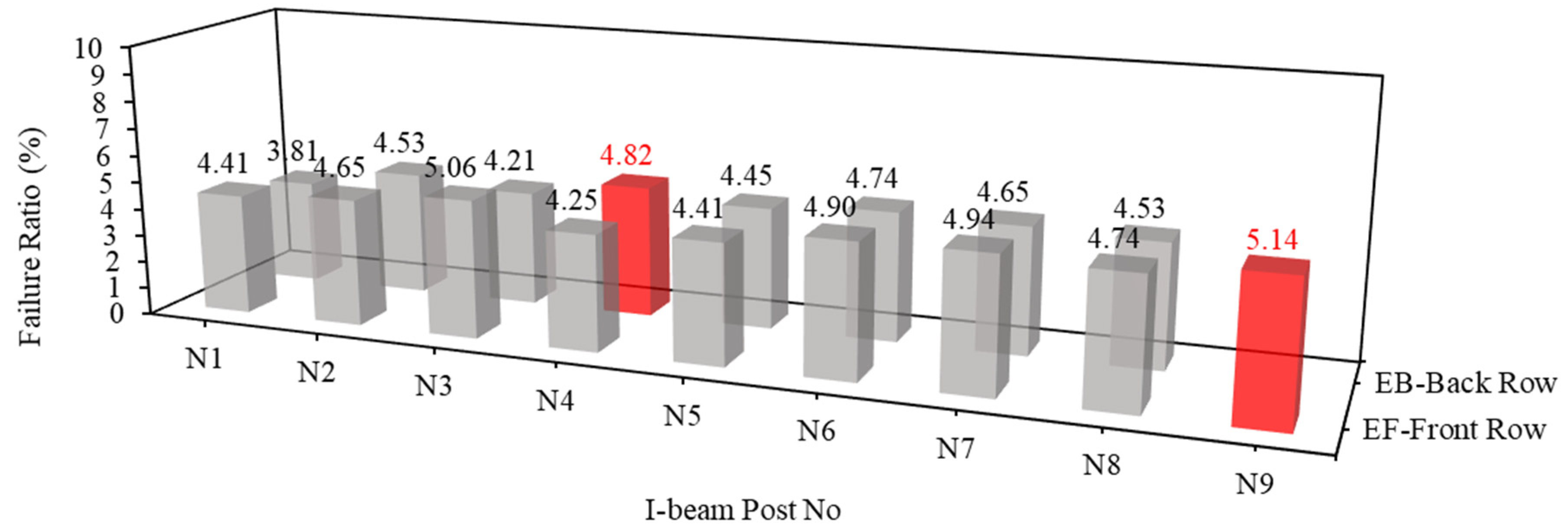
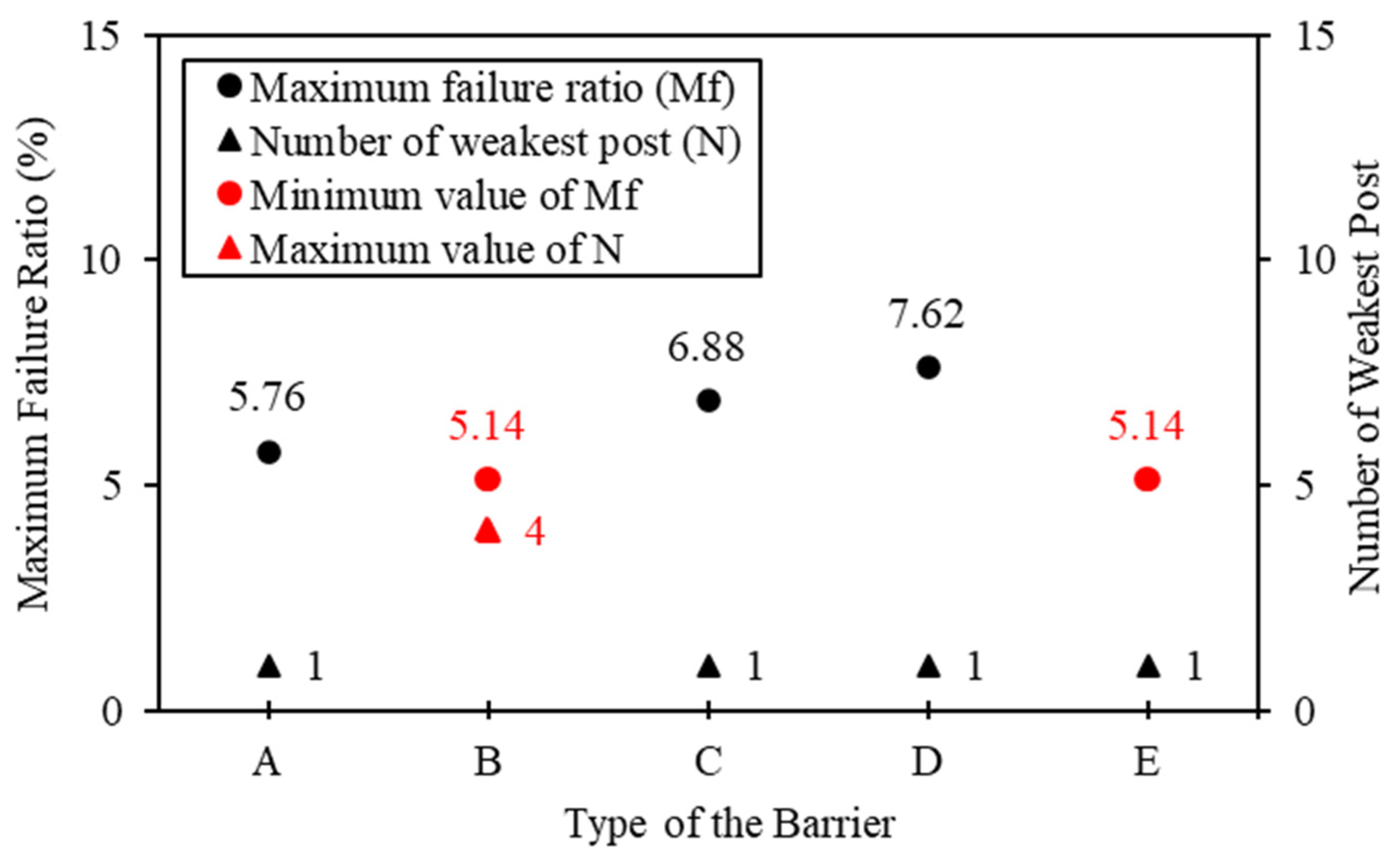
- The assessment of I-beam post efficacy against boulder impacts introduces a critical metric, the failure ratio, which quantifies the proportion of elements within the barrier that fail during impact. Based on systematic simulation and analysis, the results highlight the weakest posts within each type of I-beam barrier, underscoring the importance of identifying vulnerabilities in protective systems. While type B and type E barriers exhibit the lowest maximum failure ratios with a value of 5.14%, type E barriers demonstrate a fewer number of weakest posts, suggesting superior resilience compared to the other four types of barriers in simulation tests. Factors such as beam thickness, design characteristics, arrangement of supporting flanges, and material properties contribute to the efficacy of type E barriers. Nonetheless, it is constrained by specific site conditions and simplifications, highlighting the need for future research to refine models and consider diverse environmental factors.
Author Contributions
Funding
Data Availability Statement
Conflicts of Interest
References
- Thouret, J.-C.; Antoine, S.; Magill, C.; Ollier, C. Lahars and debris flows: Characteristics and impacts. Earth Sci. Rev. 2020, 201, 103003. [Google Scholar] [CrossRef]
- Volkwein, A.; Schellenberg, K.; Labiouse, V.; Agliardi, F.; Berger, F.; Bourrier, F.; Dorren, L.K.; Gerber, W.; Jaboyedoff, M. Rockfall characterisation and structural protection—A review. Nat. Hazards Earth Syst. Sci. 2011, 11, 2617–2651. [Google Scholar] [CrossRef]
- Li, X.; Zhao, J.; Kwan, J.S. Assessing debris flow impact on flexible ring net barrier: A coupled CFD-DEM study. Comput. Geotech. 2020, 128, 103850. [Google Scholar] [CrossRef]
- Kefayati, G.; Tolooiyan, A.; Dyson, A.P. Finite difference lattice Boltzmann method for modeling dam break debris flows. Phys. Fluids 2023, 35, 013102. [Google Scholar] [CrossRef]
- Ramachandran, V. Failure Analysis of Engineering Structures: Methodology and Case Histories; ASM International: Almere, The Netherlands, 2005. [Google Scholar]
- Li, X.P.; Yan, Q.W.; Zhao, S.X.; Luo, Y.; Wu, Y.; Wang, D.P. Investigation of influence of baffles on landslide debris mobility by 3D material point method. Landslides 2020, 17, 1129–1143. [Google Scholar] [CrossRef]
- Ng, C.W.W.; Wang, C.; Choi, C.E.; De Silva, W.; Poudyal, S. Effects of barrier deformability on load reduction and energy dissipation of granular flow impact. Comput. Geotech. 2020, 121, 103445. [Google Scholar] [CrossRef]
- Shi, H.; Huang, Y.; Feng, D.L. Numerical investigation on the role of check dams with bottom outlets in debris flow mobility by 2D SPH. Sci. Rep. 2022, 12, 20456. [Google Scholar] [CrossRef]
- Chen, H.X.; Li, J.; Feng, S.J.; Gao, H.Y.; Zhang, D.M. Simulation of interactions between debris flow and check dams on three-dimensional terrain. Eng. Geol. 2019, 251, 48–62. [Google Scholar] [CrossRef]
- Shen, W.; Li, T.L.; Li, P.; Lei, Y.L. Numerical assessment for the efficiencies of check dams in debris flow gullies: A case study. Comput. Geotech. 2020, 122, 103541. [Google Scholar] [CrossRef]
- Si, G.W.; Chen, X.Q.; Chen, J.G.; Tang, J.B.; Zhao, W.Y.; Jin, K. The Impact Force of Large Boulders with Irregular Shape in Flash Flood and Debris Flow. KSCE J. Civ. Eng. 2022, 26, 4276–4289. [Google Scholar] [CrossRef]
- Sha, S.; Dyson, A.P.; Kefayati, G.; Tolooiyan, A. An Equivalent Stiffness Flexible Barrier for Protection against Boulders Transported by Debris Flow. Int. J. Civ. Eng. 2023, 22, 705–722. [Google Scholar] [CrossRef]
- Jakob, M.; McDougall, S.; Weatherly, H.; Ripley, N. Debris-flow simulations on cheekye river, british columbia. Landslides 2013, 10, 685–699. [Google Scholar] [CrossRef]
- Luo, G.; Zhao, Y.; Shen, W.; Wu, M. Dynamics of bouldery debris flow impacting onto rigid barrier by a coupled SPH-DEM-FEM method. Comput. Geotech. 2022, 150, 104936. [Google Scholar] [CrossRef]
- Liang, Z.; Choi, C.E.; Zhao, Y.; Jiang, Y.; Choo, J. Revealing the role of forests in the mobility of geophysical flows. Comput. Geotech. 2023, 155, 105194. [Google Scholar] [CrossRef]
- Han, Z.; Su, B.; Li, Y.G.; Wang, W.; Wang, W.D.; Huang, J.L.; Chen, G.Q. Numerical simulation of debris-flow behavior based on the SPH method incorporating the Herschel-Bulkley-Papanastasiou rheology model. Eng. Geol. 2019, 255, 26–36. [Google Scholar] [CrossRef]
- Liu, C.; Yu, Z.; Zhao, S. A coupled SPH-DEM-FEM model for fluid-particle-structure interaction and a case study of Wenjia gully debris flow impact estimation. Landslides 2021, 18, 2403–2425. [Google Scholar] [CrossRef]
- Guo, J.; Cui, Y.F.; Xu, W.J.; Yin, Y.Z.; Li, Y.; Jin, W. Numerical investigation of the landslide-debris flow transformation process considering topographic and entrainment effects: A case study. Landslides 2022, 19, 773–788. [Google Scholar] [CrossRef]
- Zhao, L.; He, J.W.; Yu, Z.X.; Liu, Y.P.; Zhou, Z.H.; Chan, S.L. Coupled numerical simulation of a flexible barrier impacted by debris flow with boulders in front. Landslides 2020, 17, 2723–2736. [Google Scholar] [CrossRef]
- Chehade, R.; Chevalier, B.; Dedecker, F.; Breul, P.; Thouret, J.-C. Effect of Boulder Size on Debris Flow Impact Pressure Using a CFD-DEM Numerical Model. Geosciences 2022, 12, 188. [Google Scholar] [CrossRef]
- Sha, S.; Dyson, A.P.; Kefayati, G.; Tolooiyan, A. Modelling of debris flow-boulder-barrier interactions using the Coupled Eulerian Lagrangian method. Appl. Math. Modell. 2024, 127, 143–171. [Google Scholar] [CrossRef]
- Mazengarb, C.; Rigby, T.; Stevenson, M. Geological Survey Technical Report 37: Kunanyi/Mount Wellington Debris Flow Susceptibility and Hazard Assessment; Mineral Resources Tasmania: Rosny Park, Australia, 2023. Available online: https://www.mrt.tas.gov.au/mrtdoc/dominfo/download/TR37/ (accessed on 22 July 2024).
- Stevenson, M.; Mazengarb, C.; Woolley, R. Historical Assessment of the 1872 Glenorchy Debris Flow: A Basis for Modelling the Large Debris Flow Hazard from the Wellington Range, Hobart; Mineral Resources Tasmania: Rosny Park, Australia, 2016. Available online: https://www.researchgate.net/publication/297549846 (accessed on 22 July 2024).
- Kain, C.L.; Rigby, E.H.; Mazengarb, C. A combined morphometric, sedimentary, GIS and modelling analysis of flooding and debris flow hazard on a composite alluvial fan, Caveside, Tasmania. Sediment. Geol. 2018, 364, 286–301. [Google Scholar] [CrossRef]
- Chen, X.Y.; Zhang, L.L.; Chen, L.H.; Li, X.; Liu, D.S. Slope stability analysis based on the Coupled Eulerian-Lagrangian finite element method. Bull. Eng. Geol. Environ. 2019, 78, 4451–4463. [Google Scholar] [CrossRef]
- Lin, C.H.; Hung, C.; Hsu, T.Y. Investigations of granular material behaviors using coupled Eulerian-Lagrangian technique: From granular collapse to fluid-structure interaction. Comput. Geotech. 2020, 121, 103485. [Google Scholar] [CrossRef]
- Tatnell, L.; Dyson, A.P.; Tolooiyan, A. Coupled Eulerian-Lagrangian simulation of a modified direct shear apparatus for the measurement of residual shear strengths. J. Rock Mech. Geotech. Eng. 2021, 13, 1113–1123. [Google Scholar] [CrossRef]
- Sha, S.; Dyson, A.P.; Kefayati, G.; Tolooiyan, A. Simulation of debris flow-barrier interaction using the smoothed particle hydrodynamics and coupled Eulerian Lagrangian methods. Finite Elem. Anal. Des. 2023, 214, 103864. [Google Scholar] [CrossRef]
- Wang, P.Y.; Lian, C.C.; Yue, C.X.; Wu, X.Y.; Zhang, J.M.; Zhang, K.; Yue, Z.F. Experimental and numerical study of tire debris impact on fuel tank cover based on coupled Eulerian-Lagrangian method. Int. J. Impact Eng. 2021, 157, 103968. [Google Scholar] [CrossRef]
- Major Incidents Report 2017–18, Australian Institute for Disaster Resilience, Australian Institute for Disaster Resilience. 2018. Available online: https://knowledge.aidr.org.au/media/6196/major-incidents-report-1718.pdf (accessed on 22 July 2024).
- Mazengarb, C.; Stevenson, M. Tasmanian Landslide Map Series: User Guide and Technical Methodology; Tasmanian Geological Survey; Mineral Resources Tasmania: Rosny Park, Australia, 2010. Available online: https://www.stategrowth.tas.gov.au/mrt/geoscience/engineering_geology/geological_hazards_in_tasmania/landslides/maps/tasmanian_landslide_map_series_user_guide_and_technical_methodology (accessed on 22 July 2024).
- Leonardi, A.; Pirulli, M. Analysis of the load exerted by debris flows on filter barriers: Comparison between numerical results and field measurements. Comput. Geotech. 2020, 118, 103311. [Google Scholar] [CrossRef]
- Yang, E.; Bui, H.H.; Nguyen, G.D.; Choi, C.E.; Ng, C.W.; De Sterck, H.; Bouazza, A. Numerical investigation of the mechanism of granular flow impact on rigid control structures. Acta Geotech. 2021, 16, 2505–2527. [Google Scholar] [CrossRef]
- Kang, D.H.; Hong, M.; Jeong, S. A simplified depth-averaged debris flow model with Herschel-Bulkley rheology for tracking density evolution: A finite volume formulation. Bull. Eng. Geol. Environ. 2021, 80, 5331–5346. [Google Scholar] [CrossRef]
- Chen, Y.; Zhang, L.; Wei, X.; Jiang, M.; Liao, C.; Kou, H. Simulation of runout behavior of submarine debris flows over regional natural terrain considering material softening. Mar. Georesour. Geotechnol. 2023, 41, 175–194. [Google Scholar] [CrossRef]
- Huang, Y.; Zhu, C. Simulation of flow slides in municipal solid waste dumps using a modified MPS method. Nat. Hazards 2014, 74, 491–508. [Google Scholar] [CrossRef]
- Zhu, C.; Huang, Y.; Zhan, L.-T. SPH-based simulation of flow process of a landslide at Hongao landfill in China. Nat. Hazards 2018, 93, 1113–1126. [Google Scholar] [CrossRef]
- Hussin, H.; Quan Luna, B.; Van Westen, C.; Christen, M.; Malet, J.-P.; Van Asch, T.W. Parameterization of a numerical 2-D debris flow model with entrainment: A case study of the Faucon catchment, Southern French Alps. Nat. Hazards Earth Syst. Sci. 2012, 12, 3075–3090. [Google Scholar] [CrossRef]
- Tang, J.; Cui, P.; Wang, H.; Li, Y. A numerical model of debris flows with the Voellmy model over a real terrain. Landslides 2023, 20, 719–734. [Google Scholar] [CrossRef]
- Kafle, J.; Kattel, P.; Mergili, M.; Fischer, J.-T.; Pudasaini, S.P. Dynamic response of submarine obstacles to two-phase landslide and tsunami impact on reservoirs. Acta Mech. 2019, 230, 3143–3169. [Google Scholar] [CrossRef]
- Zhu, C.; Huang, Y.; Sun, J. A granular energy-controlled boundary condition for discrete element simulations of granular flows on erodible surfaces. Comput. Geotech. 2023, 154, 105115. [Google Scholar] [CrossRef]
- Wang, F.; Wang, J.D.; Chen, X.Q.; Zhang, S.X.; Qiu, H.J.; Lou, C.Y. Numerical Simulation of Boulder Fluid–Solid Coupling in Debris Flow: A Case Study in Zhouqu County, Gansu Province, China. Water 2022, 14, 3884. [Google Scholar] [CrossRef]
- Dai, Z.L.; Huang, Y.; Cheng, H.L.; Xu, Q. 3D numerical modeling using smoothed particle hydrodynamics of flow-like landslide propagation triggered by the 2008 Wenchuan earthquake. Eng. Geol. 2014, 180, 21–33. [Google Scholar] [CrossRef]
- Ng, C.W.; Liu, H.; Choi, C.E.; Kwan, J.S.; Pun, W.K. Impact dynamics of boulder-enriched debris flow on a rigid barrier. J. Geotech. Geoenviron. Eng. 2021, 147, 04021004. [Google Scholar] [CrossRef]
- Kwan, J. Supplementary Technical Guidance on Design of Rigid Debris-Resisting Barriers; GEO Report; Geotechnical Engineering Office, HKSAR: Hong Kong, China, 2012; Volume 270.
- Song, D.; Choi, C.E.; Ng, C.W.W.; Zhou, G.G.; Kwan, J.S.; Sze, H.; Zheng, Y. Load-attenuation mechanisms of flexible barrier subjected to bouldery debris flow impact. Landslides 2019, 16, 2321–2334. [Google Scholar] [CrossRef]
- Wendeler, C.; Volkwein, A.; McArdell, B.W.; Bartelt, P. Load model for designing flexible steel barriers for debris flow mitigation. Can. Geotech. J. 2019, 56, 893–910. [Google Scholar] [CrossRef]
- Papathoma Köhle, M.; Gems, B.; Sturm, M.; Fuchs, S. Matrices, curves and indicators: A review of approaches to assess physical vulnerability to debris flows. Earth Sci. Rev. 2017, 171, 272–288. [Google Scholar] [CrossRef]
- Cui, Y.F.; Choi, C.E.; Liu, L.H.; Ng, C.W. Effects of particle size of mono-disperse granular flows impacting a rigid barrier. Nat. Hazards 2018, 91, 1179–1201. [Google Scholar] [CrossRef]
- Mazengarb, C.; Stevenso, M.D.; Knight, K. The Mt Wellington rock fall event of 8 July 2014 described: With implications for regional scale rock fall modelling in Tasmania. In Tasmanian Geological Survey Record 2015/02; Mineral Resources Tasmania: Rosny Park, Australia, 2015. Available online: https://www.researchgate.net/publication/297549847 (accessed on 22 July 2024).
- Australian Steel Institution. AS/NZS 3679. 1: 2016 Structural Steel. Part 1: Hot-Rolled Bars and Sections; Standards Australia: Sydney, Australia, 2015; Available online: https://www.steel.org.au/resources/elibrary/library/as-nzs-3679-1-2016-structural-steel-part-1-hot-rolled-bars-and-sections/ (accessed on 22 July 2024).
- ABAQUS. Abaqus Analysis User’s Guide, Version 6.14; Dassault Systèmes Simulia Corp.: Providence, RI, USA, 2014; Available online: http://62.108.178.35:2080/v6.14/books/usb/default.htm (accessed on 22 July 2024).


| Material Parameter | Debris Flow 1,2 | Barrier 1,2 | Boulder 2 | Slope/Walls/Door 1,2 |
|---|---|---|---|---|
| Constitutive model | Bingham | Rigid body | Rigid body | Rigid body |
| Density ρ (kg/m3) | 1960 | 7800 | 2800 | - |
| Viscosity (Pa·s) | 100 | - | - | - |
| Yield stress (Pa) | 100 | - | - | - |
| Material Parameter | Debris Flow | Boulder | Hobart Rivulet Terrain | I-Beam Barrier * |
|---|---|---|---|---|
| Constitutive model | Bingham | Rigid body | Rigid body | Linear elastic |
| ρ (kg/m3) | 1500 | 2880 | - | 7850 |
| Poisson’s ratio ν | - | - | - | 0.25 |
| Young’s modulus E (kPa) | - | - | - | 2 × 10⁸ |
| (Pa) | 100 | - | - | - |
| (Pa) | 100 | - | - | - |
| Geometry | Test No | Reference Size SR (m) | Volume (m3) | Mass (tons) |
|---|---|---|---|---|
 | C1 | 0.5 | 0.1 | 0.3 |
| C2 | 1 | 0.8 | 2.3 | |
| C3 | 1.5 | 2.7 | 7.6 | |
| C4 | 2 | 6.3 | 18.1 | |
| C5 | 2.5 | 12.3 | 35.3 | |
| C6 | 3 | 21.2 | 61.1 |
| Beam Type | 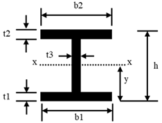 |  | |||
|---|---|---|---|---|---|
| Classification | UC150-37 | UB460-67 | UC200-18 | UC200-59 | 150PFC |
| t1 (mm) | 11.5 | 12.7 | 7 | 14.2 | 9.5 |
| t2 (mm) | 11.5 | 12.7 | 7 | 14.2 | 9.5 |
| t3 (mm) | 8.1 | 8.5 | 4.5 | 9.5 | 6 |
| b1 (mm) | 154 | 190 | 99 | 205 | 75 |
| b2 (mm) | 154 | 190 | 99 | 205 | 75 |
| y (mm) | 81 | 228.5 | 99 | 105 | 75 |
| h (mm) | 162 | 457 | 198 | 210 | 150 |
| Barrier Type | ||||||
|---|---|---|---|---|---|---|
| A | B | C | D | E | ||
| Post beam type | UC150-37 | UB460-67 | UC200-59 | UC200-59 | UC200-59 | |
| Flange beam type | UC150-37 | UB200-18 | - | 150PFC | 150PFC | |
| s1(m) | 1.2 | 1.2 | 1.5 | 1.5 | 1.5 | |
| s2 (m) | 0.6 | - | 0.9 | 0.9 | 0.75 | |
| s3 (m) | 0.78 | - | 1.4 | 1.2 | 0.95 | |
| s4 (m) | 12.65 | 12 | - | 9.205 | 12.205 | |
| s5 (m) | 0.925 | 0.6 | - | - | - | |
| s6 (m) | 1.2 | 1.2 | 1.8 | 1.8 | 1.5 | |
| s7 (mm) | 77 | 100 | - | 150 | 150 | |
| H * (m) | Minimum | 2.12 | 2.53 | 2.30 | 3.40 | 3.31 |
| Maximum | 2.80 | 3.23 | 2.72 | 3.80 | 3.78 | |
| The total length of post (m) | 51.15 | 59.94 | 30.88 | 44 | 61.42 | |
| Total length of flange (m) | 25.3 | 24 | - | 9.205 | 12.205 | |
Disclaimer/Publisher’s Note: The statements, opinions and data contained in all publications are solely those of the individual author(s) and contributor(s) and not of MDPI and/or the editor(s). MDPI and/or the editor(s) disclaim responsibility for any injury to people or property resulting from any ideas, methods, instructions or products referred to in the content. |
© 2024 by the authors. Licensee MDPI, Basel, Switzerland. This article is an open access article distributed under the terms and conditions of the Creative Commons Attribution (CC BY) license (https://creativecommons.org/licenses/by/4.0/).
Share and Cite
Sha, S.; Dyson, A.P.; Kefayati, G.; Tolooiyan, A. Analysis of Debris Flow Protective Barriers Using the Coupled Eulerian Lagrangian Method. Geosciences 2024, 14, 198. https://doi.org/10.3390/geosciences14080198
Sha S, Dyson AP, Kefayati G, Tolooiyan A. Analysis of Debris Flow Protective Barriers Using the Coupled Eulerian Lagrangian Method. Geosciences. 2024; 14(8):198. https://doi.org/10.3390/geosciences14080198
Chicago/Turabian StyleSha, Shiyin, Ashley P. Dyson, Gholamreza Kefayati, and Ali Tolooiyan. 2024. "Analysis of Debris Flow Protective Barriers Using the Coupled Eulerian Lagrangian Method" Geosciences 14, no. 8: 198. https://doi.org/10.3390/geosciences14080198