Abstract
The paper presents the author’s vision of the problem of earthquake hazards from the physical point of view. The first part is concerned with the processes of precursor’s generation. These processes are a part of the complex system of the lithosphere–atmosphere–ionosphere–magnetosphere coupling, which is characteristic of many other natural phenomena, where air ionization, atmospheric thermodynamic instability, and the Global Electric Circuit are involved in the processes of the geosphere’s interaction. The second part of the paper is concentrated on the reliable precursor’s identification. The specific features helping to identify precursors are separated into two groups: the absolute signatures such as the precursor’s locality or equatorial anomaly crests generation in conditions of absence of natural east-directed electric field and the conditional signatures due to the physical uniqueness mechanism of their generation, or necessity of the presence of additional precursors as multiple consequences of air ionization demonstrating the precursor’s synergy. The last part of the paper is devoted to the possible practical applications of the described precursors for purposes of the short-term earthquake forecast. A change in the paradigm of the earthquake forecast is proposed. The problem should be placed into the same category as weather forecasting or space weather forecasting.
1. Introduction
The problem of earthquake hazards still remains in the field of discussion and uncertainty. Several scientific communities are involved in these discussions and the field is far from consensus. One important reason is that the physical mechanism of seismogenesis has not yet been determined to the end in seismology, which leaves room for uncertainty. Thus, priority was given to statistical methods, instead of physical approaches [1]. However, the physical approach to earthquake prediction was practiced in seismology 50 years ago [2]. Unfortunately, harsh criticism of this approach led to the virtual cessation of physical precursor monitoring; instead, priority was given to statistical approaches to earthquake forecasting [3]. At the same time, measurements on artificial satellites, ground-based measurements of electromagnetic emissions and atmosphere parameters regularly demonstrated the appearance of unusual variations in the electron concentration in the ionosphere, the occurrence of electromagnetic radiation in the VLF range, anomalous propagation of radio waves, and variations in atmospheric parameters over the areas of strong earthquakes preparation [4,5,6,7]. One of the first systematizations of the ionospheric observations over earthquake-prone areas permitted the formulation of the main morphological features of the ionospheric precursors of earthquakes [8].
The first decade of the XXI century permitted us to gain the critical mass of experimental data collection concerning different types of earthquake precursors: GPS TEC [9], magnetic variations [10], atmospheric electric field variations [11], perturbations in VLF/LF electromagnetic waves propagation [12], ground surface thermal anomalies [13], OLR anomalies [14], ionospheric plasma parameters variations [15], ELF/VLF emissions in the magnetosphere [16], particle precipitations [17], and others.
Major contributions to these efforts were made by the French dedicated satellite DEMETER (Detection of Electro-Magnetic Emissions Transmitted from Earthquake Regions). It was in orbit for almost 6 years (2004–2010) and dispelled all doubts about the existence of ionospheric precursors of earthquakes and their statistical significance [18].
The second decade was marked by a sharp increase in the number of publications on earthquake precursors but, more importantly, the rising number of publications on the physical models explaining how these precursors are generated [19,20,21] and the launch of the second dedicated satellite, China Seismo-Ionospheric Satellite (CSES1), in 2018 has continued the global monitoring of the seismo-ionospheric phenomena with the great success [22].
It seems that having the physical understanding of the precursor’s generation and instruments of their registration at different levels from the ground surface to the magnetosphere in hand, we can start to use this knowledge in practical applications, including earthquake forecasts. But still, the results of the precursor’s monitoring were met with criticism and the reason for this lies in the demonstration of the precursor’s statistical reliability and detectability. That is why the recent publications on the different types of precursor registration are accompanied by the Molchan [23] and ROC (Receiver Operation Characteristic) [24] diagrams [25] and the majority of results of measurements of the cases demonstrate the high reliability of detected precursors.
Using the word “detection”, we should keep in mind that the atmosphere and ionosphere are highly variable media and that earthquake precursors could be masked by the other kinds of environmental variability such as geomagnetic storms or active solar events. Different algorithms were developed to identify the precursors under the variable background impact [26], including technologies of the precursor’s cognitive recognition [27].
Summarizing all that has been said above, one can conclude that we are ready for the real earthquake forecast but, unfortunately, this is very far from reality. In not one country is there a systemic approach to this problem. First of all, we do not have education in the field of earthquake forecasting using the physical precursors. All investigations conducted up to date are the results of the work financed from scientific grants or even performed by enthusiasts. The majority of them came from the Space Weather scientific direction. It means that we have no natural continuity of research; many results are connected with the names of individual scientists who do not have successors.
With regard to the perspective of professional seismologists, it seems that their claims on the impossibility of short-term earthquake forecasts are possibly not connected with science itself but with the fear of responsibility, the level of which is extremely high in comparison with the weather or Space Weather forecast. It seems that the paradigm of the approach to the earthquake forecast should be changed and this problem will be discussed in the last part of the paper.
2. Physics of the Earthquake Precursors in the Ionosphere
The possibility of registering from the satellite something that could be connected with earthquake preparation was initially met with hostility in the scientific community. The problem was shrouded in some mystery: how could something from underground reach cosmic space? But here, we will demonstrate that there is no mystery and that the processes involved in the precursor’s generation are characteristic of many other well-known phenomena of our environment, which should be considered as an open nonlinear system with dissipation that is described within the framework of a synergetic approach [28]. We will return to the thesis later; for now, let us consider the main physical processes responsible for the precursor’s generation.
2.1. Air Ionization
Air ionization is one of the main processes in the whole near-Earth environment because, from most distant areas of the magnetosphere up to the lower boundary of the atmosphere, we encounter ions which are the result of ionization. We can divide the sources of ionization of the atmosphere into three groups: solar electromagnetic radiation and solar wind energetic particle fluxes, galactic cosmic rays, and natural Earth radioactivity. Different altitude levels of the atmosphere are subjected to the action of different sources of solar activity and galactic cosmic rays, see Figure 1 [29].
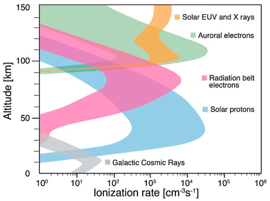
Figure 1.
Vertical profiles of ionization of the atmosphere by solar electromagnetic radiation, energetic particle fluxes, and galactic cosmic rays [29].
We can see that Galactic Cosmic Rays (GCR) having energy larger than the most energetic solar protons can penetrate up to the ground surface. A more detailed picture of the ionization of the near-ground layer of the atmosphere is presented in Figure 2 [30].
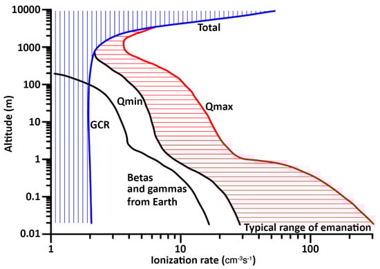
Figure 2.
Vertical profiles of air ionization from the ground surface up to 10 km altitude. Blue hatching—galactic cosmic rays; red hatching—ground radioactivity (modified from [30]).
Looking at the figure, we can conclude that the main source of air ionization near the ground surface is the natural radioactivity to which the main contribution is provided by radon [31] up to the nearly 2 km altitude where ionization effects from GCR start to prevail. To understand what effect produces the ionization in lower layers of the atmosphere, we should introduce one more that is strongly responsible for the atmosphere–ionosphere coupling: it is the Global Electric Circuit (GEC) [32]. It controls the atmospheric electricity including the potential difference between the ground surface and ionosphere and, consequently, the vertical electric current. The potential difference is created by the convective air movements and global thunderstorm activity and is of the order 250–400 kV, where the ionosphere is a positive plate and the ground surface is a negative one. In fair weather areas, the electric current is directed down, while in the area of thunderstorm activity, it is in the opposite direction. The authors of [33] analyzed the variations in the ionospheric potential (IP) due to large-scale radioactivity enhancement during nuclear tests in the atmosphere. Their model calculations demonstrated that the IP 40% increase can be explained by the 46% decrease in thunderstorm cloud conductivity. These numbers will be necessary in our following discussions. The most simplified model of GEC (but quite enough for our considerations) is presented in Figure 3.
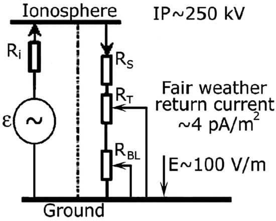
Figure 3.
Simplified model of the Global Electric Circuit.
Now, looking at this model, we can conclude that under the condition of constant current in the GEC due to current continuity, by changing the boundary layer conductivity/resistance RBL or troposphere RT, we can modulate the IP, which will lead to consequences within the ionosphere in the form of large-scale irregularities formation (negative or positive, depending on the sign of the air conductivity change) [20].
Let us return to the thesis that the mechanism of precursor generation (in our case, pre-seismic variations in the ionosphere) does not differ from other phenomena (natural or anthropogenic) where we deal with processes of air ionization. Following the model calculations for nuclear tests in the atmosphere [33], let us compare such events with the pre-seismic variations in the ionosphere. We do not have experimental data for the nuclear tests but we can use the case of the Chernobyl nuclear power plant explosion in 1986. The authors of [34] observed the anomaly of VLF signal propagation (16 kHz) registered on radio pass Rugby (Great Britain)—Kharkov (Ukraine) during the Chernobyl atomic plant catastrophe. The anomalies were registered both in amplitude and phase of the signal and they were very similar to those that are observed before strong earthquakes when the radio pass of the VLF signal is located over the earthquake preparation zone [35]. Usually, such variations are interpreted as a lowering of the upper boundary of the subionospheric resonator, which is equivalent to the increase in electron concentration in the D-layer [36]. The anomalous variations in the data around the time of the Chernobyl accident were registered even before the reactor explosion, which means that the emanation of radioactive materials started earlier. Both results are supported by the data of vertical ionospheric sounding. The main effect was observed during night-time hours, which corresponds to the formation of an earthquake precursory mask [37]. Figure 4a shows the deviation of critical frequency foF2 from the 15-day median (color coded) registered by Kiev ionosonde in coordinates Days (horizontal axis)—UTC (vertical axis). Figure 4b shows the ionospheric precursor (so-called precursor mask) obtained by the epoch overlay method for 9 earthquakes of M ≥ 5.4 in Italy at a distance of less than 300 km from Rome by the data of the Rome ionosonde. On the horizontal axis, the day’s numeration means days in relation to the earthquake day (minus—before the earthquake; plus—after it).
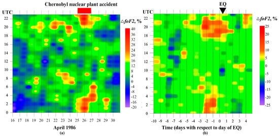
Figure 4.
(a) Deviation of critical frequency foF2 from 15-days median (color coded) registered by Kiev ionosonde in coordinates Days (horizontal axis)—UTC (vertical axis); (b) Deviation of critical frequency foF2 obtained by epoch overlay method for 9 earthquakes of M ≥ 5.4 in Italy at the distance less than 300 km from Rome by the data of the Rome ionosonde.
The similarity of two different effects, subionospheric VLF wave propagation and formation of night-time positive irregularity in the ionosphere, both for nuclear power plant accidents and for earthquakes, suggests that they have a similar or identical physical mechanism to be discussed later. We selected the anthropogenic effect for comparison but the same result can be obtained for natural phenomena such as volcano eruptions or dust storms [38,39]. Figure 5a demonstrates the ionospheric effect created by the eruption of the Kirishima volcano in Japan on 26–27 January 2011. Figure 5b demonstrates the positive variations in the ionosphere on 8 March 2011, 3 days before the M9 Tohoku earthquake.
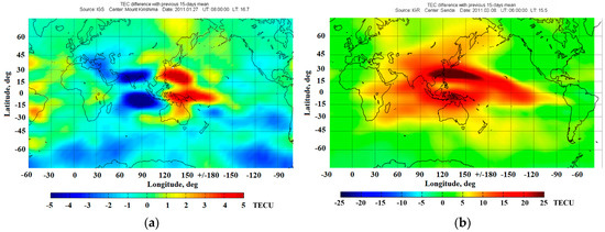
Figure 5.
(a) Differential TEC map on 27 January 2011; (b) Differential TEC map on 8 March 2011, 3 days before the M9 Tohoku earthquake. Volcano position and earthquake epicenter are shown by a white cross.
Again, the similarity of distributions demonstrated in differential TEC maps of Figure 5 is easily noticeable: in both cases, the positive deviation is concentrated at both crests of the equatorial anomaly and shifted south from the source of disturbance marked by a white cross. This effect is explained in [40] and is conditioned by the fact that, due to anisotropy of air conductivity, the vertical electric field at the ground surface is transformed in the electric field perpendicular to the geomagnetic field lines and contains components directed east. This field increases the development of equatorial anomaly and we observe the positive deviation in the differential maps. In the case of a volcano eruption, the increased electric field appears due to a voltage drop in the layer of volcano ash with very low conductivity. In case of an earthquake, the low conductivity is provided by the huge clouds of aerosol-sized cluster ions. The mechanism of their formation will be discussed in the next section. Nevertheless, in both cases, we deal with the same mechanism of electric field increase due to the low conductivity of the boundary layer of the atmosphere and troposphere.
2.2. Ion-Induced Nucleation (IIN)
In many publications estimating the effect of pre-earthquake radon emanation on the generation of earthquake precursors, only the first stage of the process is considered: air ionization by α-particles emitted by radon during its decay and consequent increase in air conductivity [41]. But the increase in conductivity of the near-ground layer of the atmosphere has a minor effect [42]. It is quite natural if we look at the Figure 3. By decreasing RBL, we leave the effect near the ground level. We have enough resistors over the boundary layer and even a strong increase in boundary layer conductivity will be limited by these resistors. In electrical engineering, they are called limiting resistors that prevent shortcuts.
Publications such as [41] do not take into account what happens after the appearance of new ions. This is described in many publications [43,44]. The initial stage of the process called ion hydration is described in [45]. The ions, immediately after their appearance, are subjected to hydration: the process of attachment of water molecules to newborn ions, Figure 6. We can see at the axis below that the process takes only 1 s.
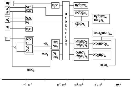
Figure 6.
Schematic presentation of the near-ground kinetics with the basic ion’s formation.
According to [46,47], the process becomes explosive and, for a short period of time, the lite ions become replaced by heavy cluster ions having extremely low mobility; hence, the conductivity of the near-ground layer of the atmosphere dramatically drops. This is confirmed by the drop in conductivity of thunderstorm clouds described in [33]. According to the same publication [33], this process increases the IP leading to the formation of large-scale increases in electron concentration or a TEC value similar to those forming over the clouds of sandstorms or volcanic ash [39].
The total vertical current I can be expressed as
where σ is air conductivity, E is the electric field, and μ is the ion’s mobility. From the discussion above, we should take into account that we have several types of ions with different sizes and, consequently, mobilities, so the integral conductivity can be expressed according to (1) as
From the Table 1, we can conclude that the ion’s mobility is also proportional to the square of the ion’s size. Two orders of magnitude ion’s size increase leads to the four orders of magnitude of the ion’s mobility drop. According to (1), we should expect a drop in air conductivity, which is proportional to mobility. But, with regard to conductivity, the amount it diminishes will depend on the balance of concentration between the light and heavy ions. In any case, an increase in heavy ions concentration in air leads to a drop in air conductivity [47], see Figure 7.

Table 1.
Variations in an ion’s mobility as dependent on the ion’s size [47].
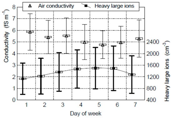
Figure 7.
Variation in concentration of heavy ions and air conductivity during a week [47].
Let us again carefully look at the Figure 3. Resistors RBL, RT, and RS are connected consecutively and each of them can play a role of the limiting resistor, as determined in electrical engineering. What does this mean? It means that if even two of them are short-circuited, the current will not go to infinity because the third limiting resistor will still exist. But in the opposite case, if the resistivity of one of the resistors increases to infinity, even if both of the others are equal to zero, the total current will be equal to zero. What consequences does it have in the case of changing conductivity in one of the layers of the atmosphere? It means that increases and decreases in conductivity are not equivalent in their consequences for the total current and ionosphere potential. Taking into account the percentage of the total resistance of the troposphere, the drop in conductivity will for sure limit the total current or, more precisely, the effect will be divided by the drop in the total current and increase in the ionosphere potential. Taking into account that during daytime aerosols (or cluster ions) spread all over the troposphere, the effect of conductivity drop will be essential.
In case conductivity increases due to the first stage of radon emanation, the effect will not be so essential because the thin layer of the near-ground matter will be subjected to this effect and yet a large part of the troposphere will remain in the previous low conductivity condition. A significant effect could be reached during the sharp explosive conductivity growth as it happens during the nuclear explosion. Both cases could be validated even without resorting to the earthquake effects.
2.3. Additional Source of GEC Modification
The major conception of GEC implies that the air conductivity is much less than the conductivity of the ionosphere and the Earth’s crust [32]; that is why only the vertical component of the electric field is registered in the atmosphere. Flowing from the ionosphere to the Earth’s ground, the current spreads over the ground surface. But this conception works only when the crust conductivity is uniform. The situation can change if the current encounters ground conductivity irregularities. In this case, we should add the crust resistance to the system of resistors in Figure 3. This is not speculation but a real experimental fact. During the last decade, geoacoustic measurements of the specific resistivity of the Earth’s crust in the deep wells (up to 3 km depth) at the Kamchatka peninsula have been provided [48]. In March 2020 when the strong M7.5 earthquake took place in northern Kurils on 25 March, synchronous measurements of the specific resistivity and GPS TEC using Petropavlovsk-Kamchatsky GPS receiver were conducted. Starting from the 16th until the 20th of March, the positive deviation of GPS TEC was registered synchronously with the increase in specific resistivity [49], which is shown in Figure 8.
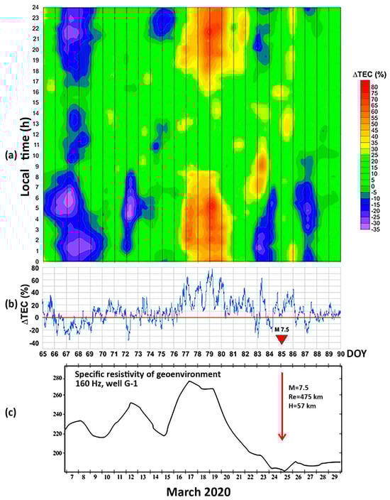
Figure 8.
(a) Percental deviation of GPS TEC at Petropavlovsk-Kamchatsky (color coded) versus local time (vertical axis), DOY (horizontal axis); (b) Time series of the DPS TEC percental deviation, a red triangle indicates the moment of the M7.5 earthquake at northern Kurils; (c) Time series of specific resistivity measured by geoacoustic emission in the G-1 deep well on frequency 160 Hz at Petropavlovsk-Kamchatsky, a red arrow indicates the moment of the M7.5 earthquake at northern Kurils.
Another effect that is frequently observed in pre-earthquake variations in atmospheric electric fields is its negative bay-like variations [50,51]. A negative direction means that the field vector is directed up, opposite to the natural electric field direction, as is shown in Figure 9. This can be reached in several ways. The simplest option is the formation of the strong electrode layer [45] when the layer of negative ions is forming over the ground surface and the electric field sensor is located under it. The electrode layer forms in any condition even without earthquakes but ionization makes it more intensive and the higher mobility of negative ions in comparison with positive ones facilitates the formation of the negative volumetric charge over the ground surface. Again, speaking of the ionization by natural radioactivity, we find similarity with man-made nuclear test activity. A few minutes after the nuclear test in the atmosphere, the negative bay in the atmospheric electric field was registered at a distance of 7.8 km from the explosion [52], see Figure 10b.
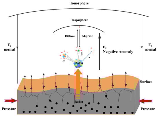
Figure 9.
Schematic diagram of atmosphere ionization by radons (after [51]).
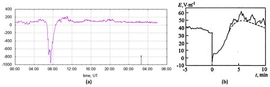
Figure 10.
(a) Negative variation in atmospheric electric field 21 h before the M5 earthquake at Kamchatka peninsula on the 24th September 1997 (vertical black arrow indicates the moment of the earthquake [51]); (b) Variation in the vertical electric field around the time of the 20 kT nuclear test in the atmosphere in 1952 [52]. Zero indicates the moment of the explosion. Bold line indicates the electric field variations, dashed line shows the trend of natural value of atmospheric electric field recovering.
The second option is the formation of a positive charge at the ground surface proposed by the peroxy defect theory [53]. It explains the possibility of moving the positive holes to the ground surface, e.g., defect electrons in the sublattice, traveling via the O 2p-dominated valence band of the silicate minerals. Regardless of the large number of publications explaining the physics of the phenomena, there are practically no experimental proofs of such effects, not to mention the statistical results.
2.4. Problems of Modeling
The problem of seismo-ionospheric coupling has a long and entangled history. First of all, it is because the majority of them have no idea of the real source leading to the variations in the ionosphere. The simplest approach is to suppose some electric field on the ground surface [53], external current [54], or surface positive charge or current [55] but nobody knows how these field, external current, or surface charge were generated. So, even if the calculations were made absolutely correctly (what never is correct to the end), we have the model without a real source directly related to the process of earthquake preparation. It looks like a castles in the air without a foundation. For the real modeling, we need the physical process generating the initial parameters used in the models mentioned above. Air ionization by radon is just a real process that is proved by many researchers, which is accepted as an earthquake precursor, and the effect of air ionization by radon is not only in atmospheric electricity but also in atmosphere thermodynamics, which will be demonstrated later.
In our LAIC model, some parts still remain on the conceptual or rush estimates level. The main problem is the correct calculation of ion kinetics in the boundary layer of the atmosphere, taking the boundary layer dynamics in local time into account. Nevertheless, the experimental results for many cases of major earthquakes convinced us that we were on the correct track. The most recent results both in theoretical and experimental proofs, which one can find in [56].
In the electromagnetic branch of our model, we use two conceptual approaches. The first one is the generation of near-ground electric field by ionization processes [45] and penetration of this field in the ionosphere [53,57]. In [57] our calculations the model value of a horizontal electric field in the ionosphere exactly corresponds to those measured experimentally onboard the FORMOSAT 5 satellite [58].
The main problem with Hegai’s model is that it does not work at equatorial latitudes. For this case, we use the second approach: modification of the air conductivity and correspondent changes in IP [39,40]. According to [59], the fair-weather current j can be estimated as
where φ∞ is the ionospheric potential IP, σ(z) is the air conductivity, and Rg is the total column resistance.
If a certain area of fair weather is exposed to aerosol-size cluster ion particles and the area of action of thunderclouds as generators of the electric field is outside the area of earthquake preparation, then, using expression (3) for the ionospheric potential, we can write the expression for the changed value of the ionosphere potential as follows:
where is the global resistance where the areas filled with the cluster ions are taken into account.
But we do not need to calculate the global resistance; we need to estimate the local variation in the IP within the specific area where the cloud of cluster ions is located.
Let us determine the regional resistance over the area S filled by cluster ions as and, from the global resistance Rg, calculate the regional resistance Rs of the same area S but without heavy ions. We obtain
where r is the radius of the Earth.
Finally, we obtain that the regional IP will be equal to
We should keep in mind that the boundary layer and troposphere practically determine the total resistance over the area and this means that the ionospheric potential over the earthquake reparation zone will be proportional to the relation between the troposphere resistance and fair-weather resistance over the same area without heavy ions.
This part of the model still lacks an approach as to how to use the IP estimated at the D-layer altitude to obtain the electron concentration in the F-layer. We are still working on this problem. Nevertheless, the similarity of results for earthquakes and areas polluted by dust storms or volcano ash convinces us that we deal with the same physical mechanism of air conductivity variations in troposphere.
Taking into account the limited volume of the paper, I will not touch upon the modification of magnetospheric tubes and conjugated VLF emissions stimulating particle precipitation. I direct the readers to our previous publications [45,60].
2.5. Effects in the E-Region of the Ionosphere
From the point of view of electric field penetration into the ionosphere, the E-layer, which is 150–200 km lower in relation to the ground surface, is more susceptible to pre-earthquake electromagnetic impacts. That is why the effects of the Chernobyl emergency were registered both in the lower ionosphere [36] and in the F-region (Figure 4a) while the Fukushima emergency effects were registered only in E-layer [61], Figure 11. Because the GPS TEC measurements are not sensitive to this region of the ionosphere, the main source of information on the pre-earthquake effects in the E-layer is data of vertical ionospheric sounding. To reveal the Fukushima explosion effects, we used the parameter called the semi-transparence coefficient of the sporadic E-layer, which is shown by blue columns in the Figure 11.
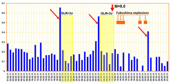
Figure 11.
Variations in the semi-transparence coefficient of the sporadic E-layer ΔfbEs around the time of the Tohoku M9 earthquake on 11 March 2011 and after explosions at Fukushima NPP. The maximal peaks of ΔfbEs are marked by burgundy arrows.
According to [62], the coefficient ΔfbEs, reflecting the effect of turbulization of the sporadic Es layer, can be expressed as
where fbEs and foEs are the screening and critical frequencies of Es.
In Figure 11, the daily mean values of ΔfbEs variations are demonstrated for the period from 1 February until the end of March 2011. During this period, we see three extremums of ΔfbEs marked by burgundy arrows. The first two coincide with the start of the period of thermal precursors of the Tohoku earthquake arising in the form of OLR emission, while the third one appears after the series of explosions at Fukushima NPP. This is one more confirmation that the observed effects are connected with air ionization from different sources but with the same physical mechanism and not any external currents proposed in the cited models.
One of the remarkable effects observed before earthquakes was described first in [63]. The authors proposed the physical mechanism of the formation of the layers of metallic aerosols at altitudes slightly higher than a normal altitude of Es due to the penetration of the seismogenic electric field. One of the recent examples of such an effect is demonstrated in Figure 12 [49] and was registered by the Petropavlovsk-Kamchatsky vertical ionosonde before the M7.5 earthquake on 25 April 2020 at northern Kurils.
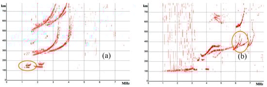
Figure 12.
(a) Formation of elevated Es at 120 km altitude (orange oval) in comparison with (b) Es normal position at 100 km altitude [49].
The observed effect was confirmed by more extended and comprehensive model calculations [64].
2.6. Summary of the Electromagnetic Branch of the LAIC Model
The discussion presented in the previous sections aimed to demonstrate that only the effect of air ionization can provide the foundation to explain all of the complex phenomena observed in all layers of the ionosphere, which are interpreted as short-term earthquake precursors. These effects have the same nature as other natural and anthropogenic phenomena arising under the action of ionization. Different sources of ionization exist and among them, radon is responsible for the generation of the chain of processes leading to the formation of ionospheric precursors. The most important conclusions are the following:
- Ions created by radon ionization and consequent ion’s hydration locally modify the GEC parameters, which leads to the generation of atmospheric electric field (positive and negative depending on atmospheric conditions) and air conductivity (increasing or decreasing with time due to ion’s hydration);
- These processes change the conditions for the subionospheric propagation of VLF waves mainly by increasing the electron concentration in the D-layer of the ionosphere, which is detected by variations in amplitude and phase of VLF signal, mainly during night-time and sunrise-sunset conditions;
- Seismogenic electric field penetrating in the E-layer of the ionosphere creates additional sporadic layers of metallic ions at altitude ~120 km and provides turbulization of the ionosphere detected by the semi-transparency coefficient ΔfbEs;
- By modification of atmospheric electric field and air conductivity, the large-scale irregularities of electron concentration (positive and negative) are formed in the F-layer of the ionosphere through changes in the IP over the earthquake preparation zone;
- Large-scale irregularities modify the geomagnetic tube loaned on this area. The stretched irregularities of electron concentration are formed along the tube where the VLF emissions are scattered and due to the increased level of VLF emission, they more effectively interact through the cyclotron resonance with energetic particles of radiation belts, which causes the stimulated particle precipitation;
- In the present moment, two approaches are used to model the F-layer effects: seismogenic electric field penetration (for high and mi-latitude ionosphere) and IP variations due to air conductivity changes for low latitudes. The model waits for future improvements;
- The model of near-ground ion kinetics still waiting for its development.
3. Physics of the Pre-Seismic Thermal Anomalies
In the previous paragraph, we demonstrated how the effects of ionization produce large-scale irregularities in the ionosphere. We proposed radon as the main agent of these irregularities’ initiation. Regardless of existing publications neglecting the possibility of radon effects on the ionosphere [41,65], we have the most powerful proof of the importance of radon as the source of the earthquake precursors: it is the thermal effects that are also the consequences of the air ionization together with the ionospheric ones. The high correlation between radon variations and large-scale pre-seismic effects in the atmosphere and the direct cause–effect relationship will be demonstrated in this paragraph.
3.1. Air Ionization Latent Heat Release and Atmosphere Reaction
The first description in our LAIC model development of the processes produced by radon ionization and subsequent hydration was described in [45] but thermal effects were not yet clearly emphasized there. A more detailed description was made in [20,56] where the high energy effectiveness was demonstrated and we will take some information from there with some modifications.
The latent heat of water evaporation per molecule (chemical potential and work function of the droplet) can be estimated from the evaporation heat Q = 40,683 kJ/mol at boiling point (T = 100 °C) U0 = Q/NA = 0.422 eV where NA = 6.022 1023/mol. So, during condensation, every molecule changing its phase state from free to bonded in a water droplet emits 0.422 eV of latent heat. Hydration is not equivalent to condensation because water molecules become attached to the ion through electrostatic attraction but still change their phase state and also emit latent heat. The theoretical consideration [56] confirmed by experimental measurements shows that in the case of hydration, the water molecule emits a larger amount of latent heat (later we will demonstrate this difference).
Radon (here we mean the main isotope Rn222) decays in the following reaction:
86Rn222 → 84Po218 + 2He4 + 5.49 MeV
In turn, polonium also emits the α-particle with an energy of 5.99 MeV
84Po218 → 82Pb214+ 2He4 + 5.99 MeV
It means that every atom of Rn222 in the result of double decay produces 11.48 MeV, which can be spent for air ionization. Taking into account that the ionization potential of air molecules is between 10 and 30 eV, every radon decay produces 5 ÷ 6 × 10⁵ ion–electron pairs.
If taking radon activity, which is usually measured in the seismically active areas of the order of ~2000 Bq/m3, then, in view of the ionization capacity of radon α-particles of ~3 × 10⁵ electron–ion pairs, the ion-formation rate is ~6 × 10⁸ m−3 s−1. A hydrated ion of a size of around 1–3 μm (particles of this size range are observed by the AERONET network a few days before the earthquake) contains around 0.4 × 10¹² water molecules. The latent heat constant U0 is U0 ~40.68 × 10³ J/mole (1 mole = 6.022 × 10²³).
For a given radon activity and the formation of hydrated ions of a size of ~1 μm, we obtain the release of latent s ~16 W/m2, which is consistent with experimentally recorded fluxes of outgoing longwave infrared radiation [14]. Since 1 eV = 1.6 × 10⁻¹⁹ J, a given radon activity of 2000 Bq/m3 leads to an expenditure on ionization of 1.7 × 10⁻⁹ J/m3 s. The ratio of IIN-induced heat to the energy spent on the ionization of atmospheric gases is then 16/(1.7 × 10−9) ~ 1010, which is evidence that the energetic efficiency of the process is extremely high.
According to [46], the H3O+(H2O)n complex ions named hydronium formed as a result of IIN playing the role of catalyzer; the process looks like an autocatalytic reaction producing more and more cluster ions capturing the water molecules from the air. We called this process thermodynamic instability [66] because we deal with the autocatalytic exothermic reaction with the transformation of energy and fast transition of water molecules from one phase state to another, which violates the thermodynamic equilibrium and leads to the formation of large-scale meteorologic anomalies in air temperature, relative humidity, and pressure.
Let us discuss what effects we may expect that accompany the latent heat release.
- Increase in the air temperature;
- Drop of relative humidity;
- Drop of air pressure due to drop of partial pressure of the water vapor.
The last point was not considered in many publications. But according to Dalton’s law, the total atmospheric pressure is the sum of the gas constituents’ pressures. Here we can consider the sum of dry air pressure and the water vapor pressure. If we are able to register all three cases of air parameters variations, it means that we are on correct track. Figure 13 shows variations in all three parameters variations from 24 February to 20 March 2022 around the time of the M7.3 Fukushima earthquake on 16 March 2022 near the east coast of Honshu Island, Japan.
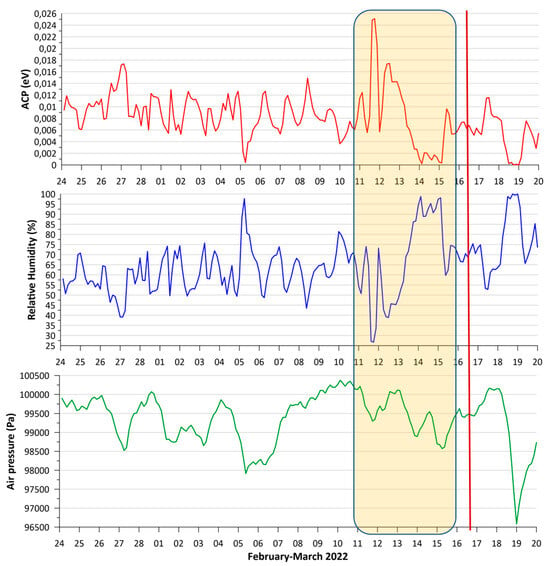
Figure 13.
From top to bottom: air temperature, relative humidity, and air pressure over the epicenter of the M7.3 Fukushima earthquake. Coordinates of the epicenter: Lat 38.23° N and Lon 141.77° E. Shadowed rectangle is the precursory period; burgundy line marks the moment of the earthquake.
It should be noted that the negative variations in the air pressure are not too prominent because of the fact that we deal with the drop of partial pressure of water vapor, and the figure reflects variations in the total air pressure. Sometimes the pre-earthquake air pressure drop is so intensive that has a blocking character for regional air movements [67].
Here may arise a question: how can we prove that the observed variations have a relation to the impending earthquake? The answer is the following: all unusual variations in environment parameters participating in the earthquake preparation process are observed within the earthquake preparation zone [68] radius, of which R is determined as
where M is the earthquake magnitude [68].
R (km) = 100.43M
As proof, we demonstrate in the Figure 14 the map of the air relative humidity (a) and air pressure (b) for measurements taken within the precursory time interval for the same M7.3 earthquake in Japan on 16 March 2022.
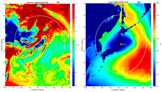
Figure 14.
(a) Relative humidity map; (b) Air pressure map.
The small size of the relative humidity drop area is probably a precursor of the Fukushima earthquake foreshock with a smaller magnitude of M6.0.
3.2. Atmosphere Chemical Potential (ACP) as an Integrated Diagnostic Parameter
The main advantage of understanding thermal precursors of earthquakes was the introduction of the conception of atmospheric chemical potential [20]. Regardless of the meteorologic parameters that demonstrate their reaction to the process of earthquake preparation, they belong to the system of global atmospheric circulation and weather anomalies. It was necessary to find parameters that, on the one hand, reflected the pre-seismic variations in atmospheric parameters and, on the other hand, were connected with some process in the Earth’s crust. The studies of the ion kinetics under action of ionization [69] demonstrated that the bond energy of the water molecule connection with the ion (chemical potential) is larger than the bond energy of the water molecule with the water drop (latent heat constant 0.422 eV). Even more, they released the dependence of the bond energy of connection with ions on the ion production rate and on the concentration of ions [20]. It means that there appeared an opportunity to estimate the intensity of ionization through the chemical potential of the water molecule attached to the ion. One more advantage is that in a moment of condensation/evaporation or attachment/detachment in reaction with an ion, the chemical potential of the water molecule equals the latent heat, which can be expressed through the atmospheric parameters (air temperature and relative humidity). It appeared that the most informative parameter is the difference in the latent heat per water molecule (or chemical potential of a water molecule) between the chemical potential of a water molecule connected with an ion and the chemical potential of connection with a water drop using the possibility to express the chemical potentials through the latent heat [20]. This parameter was called the correction of the water vapor in the atmosphere’s chemical potential. To shorten this term, in further publications, we started to use the term Atmospheric Chemical Potential (ACP). To not repeat the full derivation here (it is possible to find it in {20, 56]), we provide the final formula of the ACP as follows:
where ACP is in eV, Tg (ground temperature) in °C, and H (relative humidity)—in %.
ACP = 5.8 × 10⁻¹⁰(20Tg + 5463)2ln(100/H)
Several years of exploring ACP in earthquake precursor monitoring demonstrated its high effectiveness and established its main advantages, as follows:
- It can be used as a proxy of radon activity [56];
- It has a high correlation with the shear traction, i.e., can indicate the level of tectonic activity [66];
- Instead of traditional point measurements of radon activity, we can now track its spatial distribution and estimate the size of the earthquake preparation zone.
Continuing the presentation of Fukushima M7.3 earthquake precursor monitoring, in Figure 15a, we present a correlation between the shear traction assimilative model (red curve) and ACP (clue curve). Figure 15b shows the long-term correlation between the shear traction (rose-shadowed contour) and ACP (blue curve).
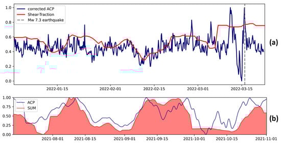
Figure 15.
(a) Average of near- and intermediate-field of ACP (corrected for pressure changes—blue) and shear-traction field (red) in the epicentral area of the 16 March 2022, Fukushima, Japan, earthquake (time shown with grey vertical line). The ACP follows the temporal evolution of the shear-traction field before the earthquake, while the spike in ACP happens close to the increase in shear-traction; (b) Long-term correlation between shear-traction field assimilative model in rose and atmospheric chemical potential (ACP) in blue, close to the Andreanof Islands, Alaska, USA.
The ACP spatial distribution before the Fukushima earthquake at 0600 UTC on 11 March is shown in Figure 16. We can see that the increased level of ACP from burgundy to light green color with yellow splashes is inside the Dobrovolsky earthquake preparation zone shown by the white circle. A strong anomaly outside the preparation zone in the north-west is the thermal wave from China, which means that ACP should be calibrated for different geographic areas. The blue arc passing through the epicenter follows the Japan trench passing into the Kuril-Kamchatka trench in the north-east.
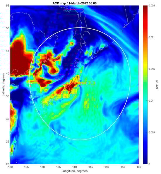
Figure 16.
Map of ACP spatial distribution within the zone of Fukushima M7.3 earthquake preparation acquired on 11 March 2022, 5 days before the earthquake.
3.3. Effects of Ionization from Other Sources (Chernobyl NPP and Fukushima NPP Emergencies)
As was mentioned in the Introduction, the effects of ionization are not unique for earthquakes and radon as a source but are the same for any source of ionization. The simplest way to check is again to study thermal effects as results of emergencies at Chernobyl 1986 and Fukushima 2011 emergencies. Figure 17 shows atmospheric parameters measured over the Fukushima NPP in March 2011.
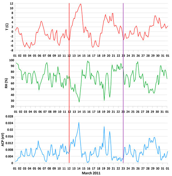
Figure 17.
From top to bottom: air temperature, relative humidity, and ACP over Fukushima NPP in March 2011. Vertical lines indicate the period of explosions.
The initial release of radioactive substances into the atmosphere occurred from March 12 to 14 and was caused by the release of pressure from the containment and explosions at blocks No. 1 and 3 [70]. This is clearly seen in Figure 17 for all parameters. We see an increase in the air temperature, a drop in relative humidity, and an increase in ACP. Other variations relate to consequent explosions at different reactors.
The power of ACP was demonstrated in the Chernobyl case and was described in [71]. The French company Institute for Radiation Protection and Nuclear Safety made measurements and modeled the dynamics of propagation of the radioactive Cs137 cloud in Europe in the form of a movie [72]. Taking into account the fact that we cannot insert the movie in the publication, we took one frame from this movie and compared it with the ACP distribution calculated for the same day. This comparison is presented in Figure 18. The position of Chernobyl NPP is shown by a yellow star. The high similarity is observed while comparing the distributions. Some details are connected by red arrows to underline this similarity. This figure confirms the power of ACP as an instrument of environment monitoring when, 36 years after the catastrophe, we are able to reconstruct the physical phenomena in detail and dynamics. This case confirms once more that the effects we observe before earthquakes have the same physical mechanism of radiation impact on the atmosphere.
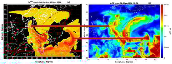
Figure 18.
(a) Spatial distribution of Cs137 on 6 May 1986 at 12:00 UTC; (b) Spatial distribution of ACP on 6 May 1986 at 12:00 UTC. Asterisks show the position of Chernobyl NPP and arrows and ovals show similarities in distributions.
3.4. Summary of the Thermal Branch of the LAIC Model
In paragraph 3, we presented the physical mechanism of the effects of ionization produced by radon emanation in the atmosphere. This is the process of energy extraction from the atmosphere due to launching the exothermic autocatalytic reaction. It should be underlined that regardless of the large individual energy of α-particles emitted by radon, in general, it is negligible in comparison with energy, which is released after the launch of this reaction. This is the main point which (if not considered) leads many authors to neglect radon impacts as the main agent of earthquake precursors generation to the wrong conclusion. We do not describe other types of thermal effects before the earthquake here [56] because they are derived from the main source—radon emanation and primary latent heat release.
The LAIC model is a multi-branch composition of many processes/precursors that were described in our previous publications [20,21,56]. The task of this paper is to provide the main physical background for precursor generation initiation. The main consequences of ionization are the electromagnetic effects created by the local modification of GEC parameters through the modulation of near-ground air electric conductivity and generation of additional vertical electric field (sometimes leading to the overturn of the electric field in relation to its natural direction). These modifications induce the formation of large-scale irregularities in the F-layer of the ionosphere (positive and negative), the formation of additional sporadic layers in the ionosphere, and the modification of the D-layer, leading to anomalies in the propagation of VLF waves within the sub-ionospheric waveguide. The development of these irregularities leads to the modification of the magnetospheric tube in which the ELF/VLF emissions are scattered and the increased level of VLF emissions stimulates the precipitation of energetic particles from the radiation belt.
The thermal branch of the LAIC model describes the formation of large-scale atmospheric irregularities through the release of latent heat extracted from the atmosphere by the IIN process. Due to the large scale of the earthquake preparation zone, we observe not only observe small anomalies over the area of the epicenter but the large meteorological anomalies occupying thousands of square kilometers. The schematic diagram of the LAIC is presented in Figure 19.
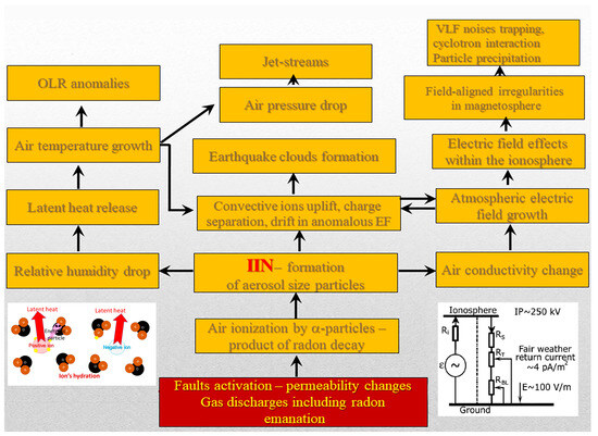
Figure 19.
Schematic presentation of the LAIC model.
4. Precursor’s Identification
In this paragraph, we will talk only about the physical precursors. Probably, the first publications determining the physical precursors were [2,73]. All of them were characterized by specific behavior during the seismic cycle and indicated the approaching of the final phase (period of short-term precursors) lasting two weeks/few days before the main event. We can mention the ground conductivity, seismic wave velocity, ground deformation, groundwater level, etc. Radon emanation also is a member of this family. Their main feature was that they were distributed within the area, which was called the “Earthquake preparation zone” by the authors [68]. This distribution has a logarithmic dependence on the magnitude of the impending earthquake (8). The dependence (8) needs explanation. The radius of the earthquake preparation zone indicates the maximal distance at which the precursors of a given earthquake can be registered but it does not mean that the whole zone should be homogeneously filled by precursors. They may appear in any place in this zone.
Radon perfectly meets these conditions. Even more, a special study of radon spatial distribution was conducted [74] and it turned out that it perfectly fits the Dobrovolsky magnitude–space relationship (Figure 20).
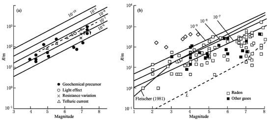
Figure 20.
(a) Determination of the size of the earthquake preparation zone in relation to magnitude according to [71]. (b) Radon and geochemical precursors of earthquake distribution versus magnitude according to [74]. The single bold line characterizes the empirical relationship of [75] who calibrated the maximum distance of a radon anomaly for a given magnitude on the basis of a shear dislocation of an earthquake. Dashed line L characterizes the typical rupture length of active faults as a function of magnitude by using the empirical law of [76]. Modified from [45].
4.1. Absolute Precursory Signatures
Here, we should determine the precursor’s features, which are absolutely necessary to be a precursor. From the introduction text of this paragraph, we already mentioned two of them: the locality of precursors (within the earthquake preparation zone) and the characteristic behavior within the seismic cycle.
One more signature follows from the physical nature of the precursor itself. It was described in [61]. For example, the equatorial anomaly in the ionosphere is formed due to the appearance of an east-directed electric field at the geomagnetic equator. This field appears in the afternoon hours of the local time and it follows that, for example, it cannot be formed during the downing hours of the local time. But before the M8.3 Illapel earthquake in Chile on 16 September 2015, the two-hump structure of the equatorial anomaly was detected by the Swarm-B satellite over the earthquake preparation zone two days before the earthquake. The same feature was regularly registered by the French DEMETER satellite at 10 LT, while the satellite passed over the preparation zone of the Wenchuan (China) M7.9 earthquake on 12 May 2008 earthquake [77].
Another property that may be classified in this category is the reaching of some environmental parameters to a magnitude that cannot be reached in natural conditions. Such an effect was registered around the time of the M6.3 earthquake close to the Chilean coast in the open ocean on 1 April 2023. The relative humidity, the drop of which is characteristic of a precursory phenomenon, reached a value 2% of what is an absolute impossible value over the open ocean.
The ionospheric precursor mask of the night-time increase in electron density in the F-layer a few days before the earthquake, demonstrated in Figure 4b and Figure 8a, is also a signature of earthquake preparation. Just this behavior of the ionosphere before the Hector Mine M7.1 earthquake in California on 16 October 1999 permitted the revelation of the ionospheric precursor in a highly disturbed ionosphere and the distinguishment of this variation from variations during the geomagnetic storm that happened a few days later [78].
The formation of an additional sporadic E-layer at an altitude of 120 km [63] is also a unique event characteristic of pre-earthquake processes.
In conclusion, we can say that absolute precursors demonstrate themselves by the unique physical characteristics not observed without earthquakes.
4.2. Precursors’ Identification
In the first decade of the XXI century when interest in ionospheric precursors grew sharply, the main technique of the precursor’s identification was statistical analysis using the interquartile range [79]. This technology has been used up to now by many researchers [80]. In addition, many other statistical technologies were proposed. As interquartile analysis, these technologies are (regardless, some of them are very sophisticated) still on the floor of usual statistics not considering the specific features of parameters connected with the earthquake preparation process and their physical nature. Nevertheless, technologies providing absolute confidence in precursor identification appeared just using the main feature of the precursor—its locality [81], Figure 21.
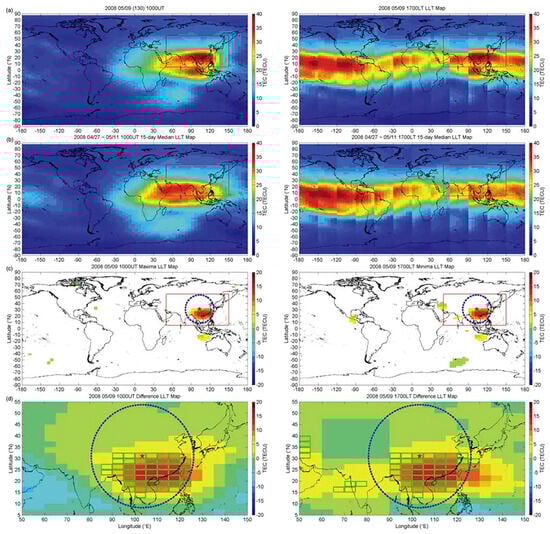
Figure 21.
(a) Left panel—UT GIM map for 1000 UT on 9 May 2009, 3 days before the Wenchuan M7.9 earthquake in China; right panel—combined LT map for 1700 LT corresponding to 1000 UT in China; (b) Left panel—15-day median GIM map for 1000 UT; right panel—combined LT map for 1700 LT corresponding to 1000 UT in China; (c) Left panel and right panel—differences between the (a,b) corresponding maps; (d) Left panel and right panel—increased images outlined by red rectangles in the corresponding images (c). Blue circle—earthquake preparation zone. At all panels red star indicates the position of the Wenchuan earthquake epicenter.
This is a very powerful and important result. First of all, this is because it undoubtedly testifies that the detected positive large-scale formation is a precursor of the Wenchuan earthquake. It demonstrates that this is a long-lived formation. This conclusion is based on the fact that the LT map has the same shape and intensity as the UT map. For the construction of an LT map, it is necessary to take several GIM maps and select the longitudinal sector corresponding to 1700 LT from them (that is why at the right panels we see the vertical strips corresponding to different GIM maps taken every 2 h). The Wenchuan precursor occupies three strips, which means that it lasts at least 6 h. Moreover, this is because the UT map occupies two time zones by 15 degrees in longitude. It confirms the possibility of constructing the maps by interpolation of data from consecutive orbits of low-orbiting satellites as we conducted topside sounding monitoring of ionospheric precursors [45]. The result perfectly shows how the Dobrovolsky earthquake preparation zone works to estimate the earthquake magnitude. And finally, it perfectly confirms the proposed physical mechanism of ionospheric precursor generation on low latitudes proposed in [40]. One can see the excitation of the equatorial anomaly: the ionospheric irregularity is located south-east from the epicenter and occupies the northern crest of the equatorial anomaly; simultaneously, the south crest of it is seen as the yellow spot at the crest latitude on the southern hemisphere. Actually, the change in the sign of electron concentration deviation was also registered in [81]: the maps are similar as in Figure 21 but 2 days earlier a negative effect was also registered and this overturn is also described in [40].
In [81], one more powerful technology is proposed based on ionospheric tomography showing the formation of additional layers at different altitudes of the F-layer. But, it needs to have a dense network of GPS receivers, which limits its application to geographic areas with such networks.
Because of growing interest in earthquake precursor studies and the corresponding volume of available information, it is possible to bring more and more recipes for precursor detection and identification. But we should remember that we deal with the nonlinear system with multivariant behavior and that obtained information is always probabilistic. Here, it can help the synergetic approach describing the system behavior in critical situations [28]. In the case of the final stage of the earthquake cycle, it manifests itself as a concentration of different types of precursors in time and space, indicating the location and time of the future seismic event [56]. That is why the only way to “catch” this process is by providing the multiparameter measurements in real-time [25,82]. This approach becomes more and more popular but it leads to an erroneous approach: registering everything you can get your hands on regardless of the physical mechanism and synergetic coupling between the precursors. We consider that only precursors with a known physical mechanism and their correspondence to the LAIC model can give a positive result; otherwise, it can lead to chaos and mistakes.
5. Practical Applications and Problems of the Earthquake Forecast
For many years now, the short-term earthquake forecast has been a painful and pressing problem. We will not start a discussion about this again; it is enough to look through the introductions to our monographs [45,56,61]. We will start from what is necessary to do.
Taking into account that our approach is based on the use of physical precursors of earthquakes, except for fundamental knowledge of seismology, we should understand the physical mechanism of precursor generation, which was the subject of previous paragraphs. Except with regard to physics, usually, the questions are raised on the precursors’ statistical reliability and credibility. For this purpose, the error diagram [23] or ROC criterion [24] are used, as was already mentioned in the Introduction. Frankly speaking, for every precursor, such a study should be performed only once to have proof of its statistical credibility because, for the real forecast, they are absolutely not necessary.
Real forecasting requires giving the answers here and now in real-time on the earthquake probability and its three parameters: time, location, and magnitude. For operative monitoring, we need to automate the process of the precursors’ registration, processing, and purification in case other factors interfere with the precursor information.
5.1. Determination of the Earthquake Parameters
Precursors described in previous paragraphs give the possibility of determining all three parameters of earthquakes with reasonable accuracy. We prepared the synthetic figure demonstrating different possibilities to determine the earthquake location and magnitude using different types of precursors and the Dobrovolsky relationship (Figure 22).
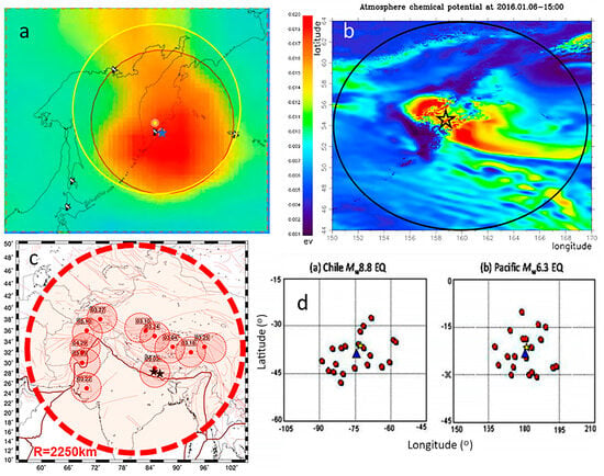
Figure 22.
(a) Differential GIM TEC map registered 4 days before the Kamchatka M6.9 earthquake on 3 March 2023. Epicenter position is marked by a yellow spot, software detected epicenter position is marked by blue star; (b) ACP spatial distribution for Kamchatka M7.2 earthquake registered a few weeks before the main shock on 30 January 2016, Dobrovolsky zone is marked by black oval; (c) The series of OLR thermal spots positions (small circles) registered before the Nepal M7.8 earthquakes in 2015; black stars indicate positions of the Nepal M7.8 earthquakes on 25 April and 17 May 2015 [83], Dobrovolsky zone is marked by red circle; (d) Distribution of electron concentration large deviations along the DEMETER satellite orbits before the Chile M8.8 earthquake on 27 February 2010 and the Chile M6.3 earthquake on 19 November 2007; red circles indicate the ionospheric anomalies detected by DEMETER satellite while passing over the earthquake preparation zone, blue triangles indicate the position of epicenter determined automatically by the data processing software, yellow stars indicate the real epicenter position [84].
Figure 22 presents precursory spatial distributions acquired by different technologies and the different precursors. Figure 22a demonstrates the result of semi-automatic processing of differential GIM maps at the Kamchatka region. The software automatically detected the epicenter (blue star) and outlined the earthquake preparation zone (burgundy circle) and the real parameters of the earthquake are shown in yellow color. Figure 22b shows the results for the same Kamchatka region but with the use of the ACP parameter. The more complex picture is presented in the Figure 22c [83]. It shows the movements of OLR precursor spots with a time of approaching Nepal 2015 M7.8 earthquakes. The earthquake epicenters are marked by black asterisks. It can be associated with the movement of a strange attractor while approaching the critical point. As was mentioned in the discussion of Figure 21, the lifetime of ionospheric precursors is long enough to be registered by several consecutive passes of the low-orbiting satellite. It gives the opportunity to outline the area of earthquake preparation from several passes as it was conducted by the DEMETER satellite [84]. More detailed analysis of DEMETER data [85] confirmed our result that that the maximum affected area in the ionosphere does not coincide with the vertical projection of the epicenter of the impending earthquake and is shifted toward the equator in low and middle latitudes as one can see in Figure 21.
Several factors reduce the accuracy of the epicenter location determination:
- 4.
- The large size of the earthquake preparation zone and the fact that the precursor may appear at any point in this zone. If taking into account that for the M7 earthquake the Dobrovolsky radius is 1000 km, the error can be quite significant;
- 5.
- The equatorward shift of ionospheric precursors for the low and middle-low latitude events where the geomagnetic field lines inclination should be considered;
- 6.
- The low spatial resolution of satellite techniques of monitoring. It is a very rare occasion that the low-orbiting satellite passes exactly over the earthquake epicenter. For OLR measurements, the anomaly location is determined within the circle of 2.5°, which is too much for the desired accuracy of 50 km.
Here, the fusion of physical precursors with seismology may help to monitor the areas with the Gutenberg–Richter relationship b-value drop [21].
As concerns the time of the earthquake, this information can be extracted from data of statistical processing. But there are two different types of statistics: the first one is for fixed sites, for example, Taiwan [9], and the second one is global, which is possible only with the help of satellite measurements [84]. Of course, if taking into account the earthquake magnitude, the distance of the GPS receiver to the epicenter, or the longitudinal distance of the satellite orbit to the epicenter, the distributions of precursors become more complex and multidimensional [85]. Nevertheless, as a result of the more comprehensive analysis of the DEMETER satellite data, the statistically most probable leading time of ionospheric precursors for earthquakes M > 5 was determined as 5 days (Figure 23a) [86], which was established as early as 1998 [45]. The first years of Langmuir probe statistical data processing at the China Seismo-Electromagnetic Satellite CSES 1 launched in 2018 gave the same 5 days of leading time, which [87] makes us more than confident that this is the most probable value for the earthquake time forecast using the ionospheric precursors (Figure 23b).
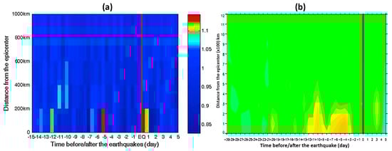
Figure 23.
(a) Statistical distribution of the number of registered ionospheric signals as a function of time in relation to the day of earthquake and distance of satellite orbit from the epicenter for the DEMETER satellite (5426 earthquakes M > 5) [86]; (b) Statistical distribution of the number of registered ionospheric signals as a function of time in relation to the day of earthquake and distance of satellite orbit from the epicenter for the CSES 1 satellite [87].
It should be noted that the leading time of different types of precursors is different, which can be used for the purpose of multiparameter monitoring. For example, the leading time of thermal precursors, including ACP, is larger than ionospheric ones [14].
It is quite natural to put the following question forward: how accurate are the earthquake parameters obtained using the proposed technologies and how large is the percentage of false alarms? These questions, up to now, have no definite answer. It is necessary to organize the real-time continuous monitoring of precursors described above, which was never performed up to now. The only exception are the data of DEMETER and CSES 1 satellites but they also have a limitation: it was not real-time but post-event analysis. In addition, we should underline that both DEMETER and CSES-1 statistics are limited by the local time of the solar synchronized orbits of both satellites: 10 AM and 10 PM for DEMETER and 2 AM and 2 PM for CSES-1. What happened at other local times remains the secret. What we need to undertake to correct this situation will be discussed in the last paragraph.
5.2. Data Purification from Other Types of Variations in Atmosphere and Ionosphere to Reveal the Earthquake Precursors
In the first 4 paragraphs, the reader accepted information not only on the physical aspect of their generation but also on how these precursors look in different ways of their presentation. A lot of publications exist on the earthquake precursors, adding that they were registered and studied in quiet solar and geomagnetic conditions. It looks like parents protect their children from any complexities of real life and they will go out into independent life infantile and helpless. If we are talking about the real earthquake forecast, we should be ready to recognize precursors at any time and in any geophysical condition.
Let us consider the main factors that interfere with physical processes generating precursors. Let us consider the interfering factors from the ground surface to the upper layers of the ionosphere and magnetosphere. Usually, there is calm weather before earthquakes but in stormy areas, such as the Pacific near the Kamchatka peninsula, the series of cyclones can blow away the radon that happened before the M7.5 earthquake east of the Kuril Islands on 25 March 2020 and we were not able to register the ACP over the epicenter. Geomagnetic storms usually change conditions of propagation of electromagnetic waves and in data of VLF signals propagating in subionospheric waveguide appear anomalies, similar to the pre-earthquake effects. During geomagnetic storms, the additional sporadic layers in E-regions of the ionosphere could form, which could be confused with the pre-earthquake sporadic layers. Simultaneously geomagnetic storms create positive and negative anomalies in the F-layer depending on the phase of the geomagnetic storm, which also interferes with the pre-seismic effects. Sharp changes in the short-ultraviolet radiation monitored with the help of the F10.7 index of solar activity can also suddenly increase or decrease electron concentration in the F-layer. As a result of geomagnetic storms, the energetic particles precipitate from radiative belts similar to pre-earthquake precipitations [60].
We developed different technologies of data processing permitting to sift out interferences and identify precursors. They are published in several tens of papers, some summary ones can be found in [8,45]. Here, we will mention only the main principles.
- Even a very strong earthquake is still a local event, so ionospheric effects will be observed only within the earthquake preparation zone, while the ionospheric effects of the geomagnetic storm are global;
- A geomagnetic storm, as a compelling force, increases the correlation between the remote areas of the ionosphere while pre-seismic effects increase the small-scale variability of the ionosphere;
- Strong variations in F10.7 can be filtered and the precursory variations may be identified due to their locality;
- Pre-earthquake variations in the ionosphere strongly depend on the local time (precursor mask) and are shorter than the ionospheric effects of the geomagnetic storm;
- The formation of sporadic layers at an altitude of 120 km in the E-region of the ionosphere is characteristic only to pre-earthquake effects;
- Multiparameter monitoring strongly helps to reveal precursors. Geomagnetic storms do not create thermal anomalies or variations in the relative humidity.
5.3. Cognitive Recognition and Automation of the Precursors’ Identification and Forecast
We developed several algorithms for the precursors’ recognition, which use the main principles mentioned above and are named based on cognitive recognition, because we use our knowledge of the physical mechanism of precursor generation as well as pattern recognition technique and machine learning. Below, the algorithms used for the cognitive recognition of the ionospheric precursors are numbered [27]:
- Analysis of ΔTEC (or ΔfoF2) data sets with the pattern–recognition method for the correspondence of the ionospheric precursor mask to changes in the ionosphere current over the seismically active region [37];
- Correlation analysis of arrays of the daily TEC values (or critical frequency foF2) between a pair of adjacent GPS/GLONASS receivers (or ground stations for vertical sounding of the ionosphere) [61];
- Calculation of the coefficient of regional variability of the ionosphere in the presence of a dense local network of stationary GPS/GLONASS receivers [61];
- Calculation and construction of differential maps of the global TEC ΔTECGIM to determine the position of the epicenter of the future earthquake and its magnitude [64]. If there is a dense local network of stationary GPS/GLONASS receivers, differential maps can be calculated with local data rather than GPS GIMs;
- Comparison of variations in the global TEC with the local TEC with reference to the solar activity index F10.7 [61];
- Calculation of the correction of the chemical potential of water vapor (ACP) according to the local temperature and relative humidity data to determine the time of the seismic event [20];
- Construction of maps of the distribution of the correction of the chemical potential according to the data of local temperature and relative humidity to determine the position of the epicenter of the future earthquake and to estimate its magnitude [61];
- Analysis of the dynamics of the equatorial anomaly (EA) for low-latitude earthquakes in order to detect the absolute anomaly and the longitudinal effect in the EA [40,61];
- Multiparameter analysis using operational data on other physical precursors, if there are any (radon activity, crustal conductivity, OLR, and anomalous cloud structures) [82].
All these algorithms were compiled in the common software system presented in Figure 24.
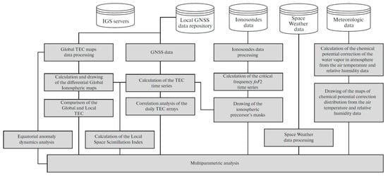
Figure 24.
Schematic diagram of the machine processing of ionosphere monitoring and space weather data for the purpose of cognitive identification of earthquake precursors.
6. Discussion and Conclusions
This publication is an attempt to present the pathway from the physical idea to the practical applications using the technologies developed during the proposed idea studies. Not one of the parts presented here does not have a finished look but there is a wise saying: “The one who walks masters the road”. But any road should have a clear goal. It can be to solve some complex problem or develop advanced technology. But some goals exist that are important to the whole of humanity and this is an earthquake forecast that we have not been able to resolve for almost two centuries. This road has bifurcation points and dead ends as in 1997 when seismologists decided that the short-term earthquake forecast was impossible [3].
Here, we try to demonstrate that the true way to the goal consists of three steps: firstly, understanding of physical background of the earthquake precursors’ generation; secondly, developing technologies for their reliable identification, and, with their help, determining the main earthquake parameters, namely time, place, and magnitude; and thirdly, in a more complex step, organization of real-time monitoring with development of the short-term forecast.
The first step was very complex. Prof. Seiya Uyeda, who left us last year, is a full member of the Japan Emperor Academy of Sciences, foreign member of American and Russian Academy of Sciences, founder of the Inter Association Working Group on Electromagnetic Studies of Earthquakes and Volcanoes (EMSEV) of IAGA/IASPEI/IAVSEI, and told me many years ago that the real earthquake forecast will be possible only after we understand the physics of the precursor’s generation. Almost 20 years passed that were spent on understanding the physics of the pre-earthquake atmospheric and ionospheric phenomena and the LAIC model [56] was created, part of which was presented in this paper.
Only after this, were we able to study the main morphological features of earthquake precursors and to develop the technologies of their definite identification.
But we cannot look at the future with optimism because the last step still looks like an impossible thing. The difficulty is not in technological problems and even not in financing: it is in human brains and politics. There is no consensus between the physicists and seismologists, the majority of whom stand on positions of the year 1997. It seems here that the problem is not only in a scientific position but also a fear of responsibility. Who will be responsible for the unfulfilled forecast and what will be the measure of responsibility? It seems that the problem can be resolved only in the way of changing the paradigm of earthquake forecast and responsibility. It should be put on the same level of responsibility as the weather forecast. It is necessary to put into the minds of the authorities that the forecast is a probabilistic value and that it can never reach 100%. We need to free seismologists from this fear and then perhaps the problem resolution will improve. The earthquake forecast should have the status of state services like medical or fire services. The earthquake forecast as a subject should be taught in universities and colleges in order to have enough specialists serving the forecast service.
Author Contributions
S.P.: Conceptualization, methodology, supervision, visualization; V.M.V.H.: Management activity, validation, review & editing, funding acquisition. All authors have read and agreed to the published version of the manuscript.
Funding
The work was carried out with the support of the Ministry of Science and Higher Education of the Russian Federation (theme/Monitoring, state registration No. 122042500031-8). Velasco Herrera thanks the UNAM Institute of Geophysics for its support.
Data Availability Statement
Data are available on request.
Acknowledgments
The authors want to acknowledge his many years of scientific collaborators: Dimitar Ouzounov, Alexander Karelin, and Valery Hegai, whose ideas and support helped to create this publication, and Pavel Budnikov who created powerful software for data processing.
Conflicts of Interest
The authors declares no conflicts of interest.
References
- Main, I. Statistical physics, seismogenesis, and seismic hazard. Rev. Geophys. 1996, 34, 433–462. [Google Scholar] [CrossRef]
- Scholz, C.H.; Sykes, L.R.; Aggarwal, Y.P. Earthquake Prediction: A Physical Basis. Science 1973, 181, 803–810. [Google Scholar] [CrossRef] [PubMed]
- Geller, R.J.; Jackson, D.D.; Kagan, Y.Y.; Mulargia, F. Earthquakes Cannot Be Predicted. Science 1997, 275, 1616–1617. [Google Scholar] [CrossRef]
- Larkina, V.I.; Migulin, V.V.; Molchanov, O.A.; Khar’kov, I.P.; Inchin, A.S.; Schvetcova, V.B. Some statistical results on very low frequency radiowave emissions in the upper ionosphere over earthquake zones. Phys. Earth Planet. Inter. 1989, 57, 100–109. [Google Scholar] [CrossRef]
- Akhmamedov, K. Interferometric measurements of the temperature of the F2 region of the ionosphere during the period of the Iranian Earthquake of June 20, 1990. Geomagn. Aeron. 1993, 33, 135–137. [Google Scholar]
- Davies, K.; Baker, D.M. Ionospheric effects observed around the time of the Alaskan earthquake of March 28, 1964. J. Geophys. Res. 1965, 70, 2251–2253. [Google Scholar] [CrossRef]
- Molchanov, O.A.; Hayakawa, M. VLF Monitoring of atmosphere-ionosphere boundary as a tool to study planetary waves evolution and seismic influence. Phys. Chem. Earth 2001, 26, 453–458. [Google Scholar]
- Pulinets, S.A.; Legen’ka, A.D.; Gaivoronskaya, T.V.; Depuev, V.K. Main phenomenological features of ionospheric precursors of strong earthquakes. J. Atmos. Sol. Terr. Phys. 2003, 65, 1337–1347. [Google Scholar] [CrossRef]
- Le, H.; Liu, J.-Y.; Liu, L. A statistical analysis of ionospheric anomalies before 736 M6.0+ earthquakes during 2002–2010. J. Geophys. Res. Space Phys. 2011, 116, A02303. [Google Scholar] [CrossRef]
- Hattori, K. ULF Geomagnetic Changes Associated with Large Earthquakes. Terr. Atmos. Ocean. Sci. 2004, 15, 329–360. [Google Scholar] [CrossRef]
- Smirnov, S. Association of the negative anomalies of the quasistatic electric field in atmosphere with Kamchatka seismicity. Nat. Hazards Earth Syst. Sci. 2008, 8, 745–749. [Google Scholar] [CrossRef]
- Hayakawa, M.; Kasahara, Y.; Nakamura, T.; Muto, F.; Horie, T.; Maekawa, S.; Hobara, Y.; Rozhnoi, A.A.; Solovieva, M.; Molchanov, O.A. A statistical study on the correlation between lower ionospheric perturbations as seen by subionospheric VLF/LF propagation and earthquakes. J. Geophys. Res. 2010, 115, A09305. [Google Scholar] [CrossRef]
- Genzano, N.; Aliano, C.; Filizzola, C.; Pergola, N.; Tramutoli, V. Robust satellite technique for monitoring seismically active areas: The case of Bhuj-Gujarat earthquake. Tectonophysics 2007, 431, 197–210. [Google Scholar] [CrossRef]
- Ouzounov, D.; Liu, D.; Kang, C.; Cervone, G.; Kafatos, M.; Taylor, P. Outgoing long wave radiation variability from IR satellite data prior to major earthquakes. Tectonophysics 2007, 431, 211–220. [Google Scholar] [CrossRef]
- Parrot, M.; Berthelier, J.J.; Lebreton, J.-P.; Sauvaud, J.A.; Santolík, O.; Blęcki, J. Examples of unusual ionospheric observations made by the DEMETER satellite over seismic regions. Phys. Chem. Earth 2006, 31, 486–495. [Google Scholar] [CrossRef]
- Němec, F.; Santolík, O.; Parrot, M. Decrease of intensity of ELF/VLF waves observed in the upper ionosphere close to earthquakes: A statistical study. J. Geophys. Res. 2009, 114, A04303. [Google Scholar] [CrossRef]
- Anagnostopoulos, G.C.; Vassiliadis, E.; Pulinets, S. Characteristics of flux-time profiles, temporal evolution, and spatial distribution of radiation-belt electron precipitation bursts in the upper ionosphere before great and giant earthquakes. Ann. Geophys. 2012, 55, 21–36. [Google Scholar]
- Parrot, M. DEMETER Satellite and Detection of Earthquake Signals. In Natural Hazards, 1st ed.; Singh, R., Bartlett, D., Eds.; Taylor & Francis Group: Boca Raton, FL, USA, 2018; pp. 115–138. [Google Scholar]
- Pulinets, S.; Ouzounov, D. Lithosphere-Atmosphere-Ionosphere Coupling (LAIC) model—An unified concept for earthquake precursors validation. J. Asian Earth Sci. 2011, 41, 371–382. [Google Scholar] [CrossRef]
- Pulinets, S.A.; Ouzounov, D.P.; Karelin, A.V.; Davidenko, D.V. Physical Bases of the Generation of Short-Term Earthquake Precursors: A Complex Model of Ionization-Induced Geophysical Processes in the Lithosphere–Atmosphere–Ionosphere–Magnetosphere System. Geomagn. Aeron. 2015, 55, 540–558. [Google Scholar] [CrossRef]
- Pulinets, S.; Ouzounov, D.; Karelin, A.; Davidenko, D. Lithosphere–Atmosphere–Ionosphere–Magnetosphere Coupling—A Concept for Pre-Earthquake Signals Generation. In Pre-Earthquake Processes: A Multidisciplinary Approach to Earthquake Prediction Studies; Ouzounov, D., Pulinets, S., Hattori, K., Taylor, P., Eds.; John Wiley & Sons, Inc.: Hoboken, NJ, USA, 2018; pp. 77–98. [Google Scholar]
- Zhima, Z.; Yan, R.; Lin, J.; Wang, Q.; Yang, Y.; Lv, F.; Huang, J.; Cui, J.; Liu, Q.; Zhao, S.; et al. The Possible Seismo-Ionospheric Perturbations Recorded by the China-Seismo-Electromagnetic Satellite. Remote Sens. 2022, 14, 905. [Google Scholar] [CrossRef]
- Molchan, G.M. Earthquake prediction as a decision-making problem. Pure Appl. Geophys. 1997, 147, 233–247. [Google Scholar] [CrossRef]
- Junge, M.R.; Dettori, J.R. ROC Solid: Receiver Operator Characteristic (ROC) Curves as a Foundation for Better Diagnostic Tests. Glob. Spine J. 2018, 8, 424–429. [Google Scholar] [CrossRef] [PubMed]
- Ouzounov, D.; Pulinets, S.; Liu, J.-Y.; Hattori, K.; Han, P. Multiparameter Assessment of Pre-Earthquake Atmospheric Signals. In Pre-Earthquake Processes: A Multidisciplinary Approach to Earthquake Prediction Studies; Ouzounov, D., Pulinets, S., Hattori, K., Taylor, P., Eds.; John Wiley & Sons, Inc.: Hoboken, NJ, USA, 2018; pp. 339–359. [Google Scholar] [CrossRef]
- Akhoondzadeh, M. Genetic algorithm for TEC seismo-ionospheric anomalies detection around the time of the Solomon (Mw = 8.0) earthquake of 06 February 2013. Adv. Space Res. 2013, 52, 581–590. [Google Scholar] [CrossRef]
- Pulinets, S.A.; Davidenko, D.V.; Budnikov, P.A. Method for Cognitive Identification of Ionospheric Precursors of Earthquakes. Geomagn. Aeron. 2021, 61, 14–24. [Google Scholar] [CrossRef]
- Knyazeva, E.N.; Kurdiumov, S.P. Peculiar properties of nonequilibrium processes in open dissipative media. In The Problems of XXI Century Geophysics, 1st ed.; Nikolaev, A.A., Ed.; Nauka Publ.: Moscow, Russia, 2003; pp. 37–65. [Google Scholar]
- Mironova, I.A.; Aplin, K.L.; Arnold, F.; Bazilevskaya, G.A.; Harrison, R.G.; Krivolutsky, A.A.; Nicoll, K.A.; Rozanov, E.V.; Turunen, E.; Usoskin, I.G. Energetic Particle Influence on the Earth’s Atmosphere. Space Sci. Rev. 2015, 194, 1–96. [Google Scholar] [CrossRef]
- Hoppel, W.A.; Anderson, R.V.; Willet, J.C. Atmospheric electricity in the planetary boundary layer. In The Earth’s Electrical Environment; National Academic Press: Cambridge, MA, USA, 1986; pp. 149–165. [Google Scholar]
- Tölgyessy, M.; Harangozó. RADIOCHEMICAL METHODS|Natural and Artificial Radioactivity. In Encyclopedia of Analytical Science, 2nd ed.; Worsfold, P., Townshend, A., Poole, C., Eds.; Elsevier: Amsterdam, The Netherlands, 2005; pp. 8–15. [Google Scholar]
- Williams, E.R.; Mareev, E. Recent progress on the global electrical circuit. Atmos. Res. 2014, 135–136, 208–227. [Google Scholar] [CrossRef]
- Slyunyaev, N.N.; Mareev, E.A.; Zhidkov, A.A. On the variation of the ionospheric potential due to large-scale radioactivity enhancement and solar activity. J. Geophys. Res. Space Phys. 2015, 120, 7060–7082. [Google Scholar] [CrossRef]
- Fux, I.M.; Shubova, R.S. VLF signal anomalies as response on the processes within near-earth atmosphere. Geomagn. Aeronom. 1995, 34, 130–135. [Google Scholar]
- Rozhnoi, A.; Solovieva, M.; Molchanov, O.; Schwingenschuh, K.; Boudjada, M.; Biagi, P.F.; Maggipinto, T.; Castellana, L.; Ermini, A.; Hayakawa, M. Anomalies in VLF radio signals prior the Abruzzo earthquake (M = 6.3) on 6 April 2009. Nat. Hazards Earth Syst. Sci. 2009, 9, 1727–1732. [Google Scholar] [CrossRef]
- Martynenko, S.I.; Fuks, I.M.; Shubova, R.S. Ionospheric electric-field influence on the parameters of VLF signals connected with nuclear accidents and earthquakes. J. Atmos. Electr. 1996, 16, 259–269. [Google Scholar]
- Pulinets, S.A.; Davidenko, D.V. The Nocturnal Positive Ionospheric Anomaly of Electron Density as a Short-Term Earthquake Precursor and the Possible Physical Mechanism of its Formation. Geomagn. Aeron. 2018, 58, 559–570. [Google Scholar] [CrossRef]
- Tramutoli, V.; Marchese, F.; Falconieri, A.; Filizzola, C.; Genzano, N.; Hattori, K.; Lisi, M.; Liu, J.-Y.; Ouzounov, D.; Parrot, M.; et al. Tropospheric and Ionospheric Anomalies Induced by Volcanic and Saharan Dust Events as Part of Geosphere Interaction Phenomena. Geosciences 2019, 9, 177. [Google Scholar] [CrossRef]
- Pulinets, S.A.; Davidenko, D.V.; Pulinets, M.S. Atmosphere-ionosphere coupling induced by volcanoes eruption and dust storms and role of GEC as the agent of geospheres interaction. Adv. Space Res. 2022, 69, 4319–4334. [Google Scholar] [CrossRef]
- Pulinets, S. Low-Latitude Atmosphere-Ionosphere Effects Initiated by Strong Earthquakes Preparation Process. Int. J. Geophys. 2012, 2012, 131842. [Google Scholar] [CrossRef]
- Denisenko, V.V.; Rozanov, E.V.; Belyuchenko, K.V.; Bessarab, F.S.; Golubenko, K.S.; Klimenko, M.V. The Ionospheric Electric Field Perturbation with an Increase in Radon Emanation. Russ. J. Phys. Chem. B Focus. Phys. 2024, 18, 837–843. [Google Scholar] [CrossRef]
- Bliokh, P. Variations of Electric Fields and Currents in the Lower Ionosphere Produced by Conductivity Growth of the Air above the Future Earthquake Center. In Atmospheric and Ionospheric Electromagnetic Phenomena Associated with Earthquakes; Hayakawa, M., Ed.; TERRAPUB: Tokyo, Japan, 1999; pp. 829–838. [Google Scholar]
- Kathmann, S.M.; Schenter, G.K.; Garrett, B.C. Ion-induced nucleation: The importance of chemistry. Phys. Rev. Lett. 2005, 94, 116104. [Google Scholar] [CrossRef] [PubMed]
- Svensmark, H.; Enghoff, M.B.; Shaviv, N.J.; Svensmark, J. Increased ionization supports growth of aerosols into cloud condensation nuclei. Nat. Commun. 2017, 8, 2199. [Google Scholar] [CrossRef] [PubMed]
- Pulinets, S.A.; Boyarchuk, K.A. Ionospheric Precursors of Earthquakes, 1st ed.; Springer: Berlin/Heidelberg, Germany, 2004; Volume 315. [Google Scholar] [CrossRef]
- Timofeev, V.E.; Grigoryev, V.G.; Morozova, E.I.; Skryabin, N.G.; Samsonov, S.N. Action of cosmic rays on the latent energy of the atmosphere. Geomag. Aeron. 2003, 43, 636–640. [Google Scholar]
- Hõrrak, U. Air Ion Mobility Spectrum at A Rural Area. Ph.D. Thesis, Tartu Ülikooli Kirjastuse, Trükikoda, Tartu City, Estonia, 2001. [Google Scholar]
- Gavrilov, V.A.; Panteleev, I.A.; Deshcherevskii, A.V.; Lander, A.V.; Morozova, Y.V.; Buss, Y.Y.; Vlasov, Y.A. Stress–Strain State Monitoring of the Geological Medium Based on The Multi-instrumental Measurements in Boreholes: Experience of Research at the Petropavlovsk-Kamchatskii Geodynamic Testing Site (Kamchatka, Russia). Pure Appl. Geophys. 2020, 177, 397–419. [Google Scholar] [CrossRef]
- Bogdanov, V.; Gavrilov, V.; Pulinets, S.; Ouzounov, D. Responses to the preparation of strong Kamchatka earthquakes in the lithosphere–atmosphere–ionosphere system, based on new data from integrated ground and ionospheric monitoring. E3S Web Conf. 2020, 196, 03005. [Google Scholar] [CrossRef]
- Smirnov, S. Negative Anomalies of the Earth’s Electric Field as Earthquake Precursors. Geosciences 2020, 10, 10. [Google Scholar] [CrossRef]
- Han, R.; Cai, M.; Chen, T.; Yang, T.; Xu, L.; Xia, Q.; Jia, X.; Han, J. Preliminary Study on the Generating Mechanism of the Atmospheric Vertical Electric Field before Earthquakes. Appl. Sci. 2022, 12, 6896. [Google Scholar] [CrossRef]
- Holzer, R.E. Atmospheric electrical effects of nuclear explosions. J. Geophys. Res. 1972, 77, 5845–5855. [Google Scholar] [CrossRef]
- Khegai, V.V. Analytical model of a seismogenic electric field according to data of measurements in the surface layer of the midlatitude atmosphere and calculation of its magnitude at the ionospheric level. Geomagn. Aeron. 2020, 60, 507–520. [Google Scholar] [CrossRef]
- Sorokin, V.; Novikov, V. A model of TEC perturbations possibly related to seismic activity. Ann. Geophys. 2023, 66, SE642. [Google Scholar] [CrossRef]
- Kuo, C.L.; Lee, L.C.; Huba, J.D. An improved coupling model for the lithosphere-atmosphere-ionosphere system. J. Geophys. Res. Space Phys. 2014, 119, 3189–3205. [Google Scholar] [CrossRef]
- Pulinets, S.; Ouzounov, D.; Karelin, A.; Boyarchuk, K. Earthquake Precursors in the Atmosphere and Ionosphere; Springer Nature: Dordrecht, The Netherlands, 2022; Available online: https://link.springer.com/book/10.1007/978-94-024-2172-9 (accessed on 30 July 2024).
- Hegai, V.; Zeren, Z.; Pulinets, S. Seismogenic Field in the Ionosphere before Two Powerful Earthquakes: Possible Magnitude and Observed Ionospheric Effects (Case Study). Atmosphere 2023, 14, 819. [Google Scholar] [CrossRef]
- Liu, J.-Y.; Chao, C.-K. An observing system simulation experiment for 1 FORMOSAT-5/AIP detecting seismoionospheric precursors. Terr. Atmos. Ocean. Sci. 2017, 28, 117–127. [Google Scholar] [CrossRef]
- Morozov, V.N. Mathematical Modeling of Atmospheric-Electrical Processes Taking into Account the Influence of Aerosol Particles and Radioactive Substances; Russian State Hydrometeorological University Publishing: Saint-Petersburg, Russia, 2011. [Google Scholar]
- Pulinets, S.; Krankowski, A.; Hernandez-Pajares, M.; Marra, S.; Cherniak, I.; Zakharenkova, I.; Rothkaehl, H.; Kotulak, K.; Davidenko, D.; Blaszkiewicz, L.; et al. Ionosphere Sounding for Pre-seismic Anomalies Identification (INSPIRE): Results of the Project and Perspectives for the Short-Term Earthquake Forecast. Front. Earth Sci. 2021, 9, 610193. [Google Scholar] [CrossRef]
- Pulinets, S.; Ouzounov, D. The Possibility of Earthquake Forecasting: Learning from Nature; IOP Publishing: Bristol, UK, 2018; Available online: https://iopscience.iop.org/book/978-0-7503-1248-6 (accessed on 30 July 2024).
- Liperovskaya, E.V.; Pokhotelov, O.A.; Hobara, Y.; Parrot, M. Variability of sporadic E-layer semi transparency (foEs − fbEs) with magnitude and distance from earthquake epicenters to vertical sounding stations. Nat. Hazards Earth Syst. Sci. 2003, 3, 279–284. [Google Scholar] [CrossRef]
- Kim, V.P.; Khegai, V.V.; Illich-Svitych, P.V. Probability of formation of a metallic ion layer in the nighttime midlatitude ionospheric E-region before strong earthquakes. Geomagn. Aeron. 1993, 33, 114–119. [Google Scholar]
- Xu, T.; Hu, Y.; Deng, Z.; Zhang, Y.; Wu, J. Revisit to sporadic E layer response to presumably seismogenic electrostatic fields at middle latitudes by model simulation. J. Geophys. Res. Space Phys. 2020, 125, e2019JA026843. [Google Scholar] [CrossRef]
- Surkov, V.V.; Pilipenko, V.A.; Silina, A.S. Can Radioactive Emanations in a Seismically Active Region Affect Atmospheric Electricity and the Ionosphere? Izv. Phys. Solid Earth 2022, 58, 297–305. [Google Scholar] [CrossRef]
- Pulinets, S.; Budnikov, P.; Karelin, A.; Žalohar, J. Thermodynamic instability of the atmospheric boundary layer stimulated by tectonic and seismic activity. J. Atmos. Sol. Terr. Phys. 2023, 246, 106050. [Google Scholar] [CrossRef]
- Daneshvar, M.R.M.; Tavousi, T.; Khosravi, M. Atmospheric blocking anomalies as the synoptic precursors prior to the induced earthquakes: A new climatic conceptual model. Int. J. Environ. Sci. Technol. 2015, 12, 1705–1718. [Google Scholar] [CrossRef]
- Dobrovolsky, I.R.; Zubkov, S.I.; Myachkin, V.I. Estimation of the size of earthquake preparation zones. Pure Appl. Geophys. 1979, 117, 1025–1044. [Google Scholar] [CrossRef]
- Boyarchuk, K.A.; Karelin, A.V.; Shirokov, R.V. Bazovaya model’ kinetiki ionizirovannoi atmosfery. In The Reference Model of Ionized Atmospheric Kinetics; VNIIEM Publ.: Moscow, Russia, 2006. [Google Scholar]
- Tsuruda, T. Nuclear power plant explosions at Fukushima-Daiichi. Procedia Eng. 2013, 62, 71–77. [Google Scholar] [CrossRef]
- Pulinets, S.; Budnikov, P. Atmosphere Critical Processes Sensing with ACP. Atmosphere 2022, 13, 1920. [Google Scholar] [CrossRef]
- Expansion of Radioactive Cloud after Chernobyl Disaster. Available online: https://www.youtube.com/watch?v=mqu_l29WioM (accessed on 6 June 2024).
- Bolt, B.A. Earthquakes: A Primer; W.H. Freeman: San Francisco, CA, USA, 1978; p. 241. [Google Scholar]
- Toutain, J.-P.; Baubron, J.-C. Gas geochemistry and seismotectonics: A review. Tectonophysics 1998, 304, 1–27. [Google Scholar] [CrossRef]
- Fleischer, R.L. Dislocation model for radon response to distant earthquakes. Geophys. Res. Lett. 1981, 8, 477–480. [Google Scholar] [CrossRef]
- Aki, K.; Richards, P.G. Quantitative Seismology. Theory and Methods; Freeman: New York, NY, USA, 1980. [Google Scholar]
- Ryu, K.; Parrot, M.; Kim, S.G.; Jeong, K.S.; Chae, J.S.; Pulinets, S.; Oyama, K.-I. Suspected seismo-ionospheric coupling observed by satellite measurements and GPS TEC related to the M7.9 Wenchuan earthquake of 12 May 2008. J. Geophys. Res. Space Phys. 2014, 119, 305–323. [Google Scholar] [CrossRef]
- Pulinets, S.; Tsidilina, M.; Ouzounov, D.; Davidenko, D. From Hector Mine M7.1 to Ridgecrest M7.1 Earthquake. A Look from a 20-Year Perspective. Atmosphere 2021, 12, 262. [Google Scholar] [CrossRef]
- Liu, J.Y.; Chen, Y.I.; Chuo, Y.J.; Chen, C.S. A statistical investigation of preearthquake ionospheric anomaly. J. Geophys. Res. 2006, 111, A05304. [Google Scholar] [CrossRef]
- Liu, J.-Y.; Hattori, K.; Chen, Y.-I. Application of Total Electron Content Derived from the Global Navigation Satellite System for Detecting Earthquake Precursors. In Pre-Earthquake Processes: A Multidisciplinary Approach to Earthquake Prediction Studies; Ouzounov, D., Pulinets, S., Hattori, K., Taylor, P., Eds.; John Wiley & Sons, Inc.: Washington DC, USA, 2018; pp. 305–317. [Google Scholar] [CrossRef]
- Liu, J.Y.; Chen, Y.I.; Chen, C.H.; Liu, C.Y.; Chen, C.Y.; Nishihashi, M.; Li, J.Z.; Xia, Y.Q.; Oyama, K.I.; Hattori, K.; et al. Seismoionospheric GPS total electron content anomalies observed before the 12 May 2008 Mw7.9 Wenchuan earthquake. J. Geophys. Res. 2009, 114, A04320. [Google Scholar] [CrossRef]
- Ouzounov, D.; Pulinets, S.; Hattori, K.; Kafatos, M.; Taylor, P. Atmospheric signals associated with major earthquakes. A multi-sensor approach. In The Frontier of Earthquake Prediction Studies; Hayakawa, M., Ed.; Nihon-Senmontosho-Shuppan: Tokyo, Japan, 2012; pp. 510–531. [Google Scholar]
- Ouzounov, D.; Pulinets, S.; Davidenko, D.; Rozhnoi, A.; Solovieva, M.; Fedun, V.; Dwivedi, B.N.; Rybin, A.; Kafatos, M.; Taylor, P. Transient Effects in Atmosphere and Ionosphere Preceding the 2015 M7.8 and M7.3 Gorkha–Nepal Earthquakes. Front. Earth Sci. 2021, 9, 757358. [Google Scholar] [CrossRef]
- Li, M.; Parrot, M. Statistical analysis of an ionospheric parameter as a base for earthquake prediction. J. Geophys. Res. 2013, 3731–3739. [Google Scholar] [CrossRef]
- He, Y.; Yang, D.; Qian, J.; Parrot, M. Response of the Ionospheric Electron Density to Different Types of Seismic Events. Nat. Hazards Earth Syst. Sci. 2011, 11, 2173–2180. [Google Scholar] [CrossRef]
- Yan, R.; Parrot, M.; Pinçon, J.-L. Statistical study on variations of the ionospheric ion density observed by DEMETER and related to seismic activities. J. Geophys. Res. 2017, 122, 12,421–12,429. [Google Scholar] [CrossRef]
- Shen, X. From CSES to IMCP. In Proceedings of the IMCP International Workshop, NSSC-Huairou Campus, Beijing, China, 14–17 September 2023. [Google Scholar]


Disclaimer/Publisher’s Note: The statements, opinions and data contained in all publications are solely those of the individual author(s) and contributor(s) and not of MDPI and/or the editor(s). MDPI and/or the editor(s) disclaim responsibility for any injury to people or property resulting from any ideas, methods, instructions or products referred to in the content. |
© 2024 by the authors. Licensee MDPI, Basel, Switzerland. This article is an open access article distributed under the terms and conditions of the Creative Commons Attribution (CC BY) license (https://creativecommons.org/licenses/by/4.0/).