Abstract
This study is aimed at a comprehensive assessment of the chemical composition of surface waters in the Turkestan region and their impact on regional landscapes. The primary objective of the research is to systematically evaluate the level of chemical pollution in the region’s water resources and determine its indirect effects on landscape-ecological stability. In August 2024, water samples from eight sampling points (S1–S8) were analyzed for 24 physicochemical parameters, including total hardness (mg*eq/L), pH, dry residue (mg/L), electrical conductivity (µS/cm), total salinity (mg/L), Al, As, B, Ca, Cd, Co, Cr, Ti, Fe, Pb, Cu, Mg, K, Mn, Na, Ni, Zn, SO42−, and C6H5OH. To determine the degree of pollution, variational-statistical analysis, principal component analysis (PCA), as well as the calculation of the OIP, NPI, and HPI indices were performed. For land use and land cover change (LULC) analysis, LULC classification was carried out based on Landsat data from 2000 to 2020, forming the basis for land resource management and planning. The research results showed a deterioration in the ecological condition of water resources and an increasing anthropogenic impact. Specifically, at point S8, the concentration of Al was found to be 56 times higher than the maximum allowable limit, while the concentration of Fe was 42 times higher. High levels of pollution were also recorded at points S1, S4, S5, and S6, where the increase in Al and Na concentrations caused a sharp rise in the OIP value. The main factors influencing water pollution include industrial effluents, agricultural waste, and irrigation drainage waters. The pollution’s negative impact on regional landscapes has led to issues related to the distribution of vegetation, soil fertility, and landscape stability. To improve the current ecological situation and restore natural balance, the phytoremediation method is proposed. The research results will serve as the foundation for developing water resource management strategies for the Turkestan region and making informed decisions aimed at ensuring ecological sustainability.
1. Introduction
Due to the increasing anthropogenic pressure and the effects of global climate change, there is a growing need to reassess the chemical pollution of surface waters, which significantly impacts the stability of landscape systems. The preservation of the natural environment and ecological balance has become a critical issue at present [1,2,3,4,5]. In recent decades, the pollution of natural water resources has intensified as a result of human economic and industrial activities [6]. Especially in arid and semi-arid regions, including the Turkestan region, the change in the chemical composition of surface water sources has indirect effects on landscape processes, making it one of the key areas for interdisciplinary research [7].
The deterioration of surface water quality disrupts biogeochemical cycles and geochemical equilibrium, negatively affecting ecological sustainability and landscape morphodynamics. The entry of pollutants (such as heavy metals and organic and inorganic contaminants) into aquatic ecosystems alters natural feedback mechanisms, damaging landscape morphology and stability [8].
The diversity of geological and hydroclimatic conditions in the Turkestan region creates complex factors that affect landscapes and ecological systems. Land use and land cover changes negatively impact the chemical quality of surface waters and influence soil properties and vegetation structure [9,10,11,12]. These processes are exacerbated by the effects of climate change, making regional landscapes more vulnerable to natural stressors [13]. Pollutants have a long-term negative impact on both aquatic and terrestrial landscapes, leading to changes in landscape structure and function.
Heavy metals, resulting from agricultural and industrial activities, enter surface waters, degrading landscapes and reducing water quality in the Turkistan region. Fertilizers and pesticides used in agriculture are washed into rivers through runoff, increasing the levels of NO3− and PO43−. This intensifies eutrophication, leading to the destabilization of aquatic ecosystems [14,15,16]. Waste from construction, industry, and livestock farming enters rivers through precipitation, further deteriorating water quality.
A systematic analysis of the dynamics of water quality and its impact on landscape stability is crucial. The distribution of pollutants alters the chemical properties of soils, the availability of nutrients to plants, and their structure, leading to significant changes in landscape morphology [17,18,19,20,21,22,23]. To ensure water quality and landscape stability, comprehensive measures must be taken.
Previously, several physicochemical and biological parameters such as total hardness, pH, dry residue, electrical conductivity, and total salinity were studied to assess water quality [24,25,26]. Various organizations have adopted indices based on mathematical and statistical methods [27,28,29]. To effectively assess the variability in heavy metals in water samples for water quality evaluation, principal component analysis (PCA) was used, employing variational-statistical indicators based on scientific principles. The overall pollution index (OIP) is applied as it reflects the cumulative effect of multiple pollutants [30]. Additionally, the Nemerov pollution index (NPI) allows for the assessment of the cumulative impact of several parameters affecting water quality [31,32,33]. The heavy metal pollution index (HPI) is used to assess heavy metal pollution, comparing the concentration of heavy metals with standard thresholds to determine their ecological impact [34]. For the analysis of the landscape features in the Turkestan region, land use and land cover (LULC) classification was performed based on satellite data from Landsat between 2000 and 2020. This method facilitates the effective management and planning of land resources.
In the Turkestan region, the presence of heavy metals such as Cd and Pb has increased the HPI value, indicating that water resources are polluted to levels that pose a health risk. Heavy metals negatively impact ecosystem stability, leading to the slowdown of natural processes and degradation [35,36,37,38,39]. Such pollution is associated with natural mineral decay, soil erosion, industrial effluents, agricultural waste, rainwater, and construction activities [40,41]. These factors degrade water quality and cause long-term damage to landscapes.
Several projects are being implemented in the Turkestan region to improve the quality of the surface waters. In 2023, major repairs were carried out on a 62-kilometer canal, and 488 kilometers of drainage systems underwent mechanical cleaning. These measures improved the meliorative condition of 19.4 thousand hectares of irrigated land. Additionally, monitoring was conducted at 143 water bodies, including 93 rivers and 31 lakes. As a result, the level of chemical pollution in the Syr Darya, Eginsu, and Katta-Bogen rivers confirmed the deterioration of water quality [42,43,44,45]. The importance of small-scale studies to identify factors affecting landscapes is increasing. Such studies help in developing measures to improve water quality and in creating pollution prevention strategies. However, despite initiatives to improve water quality in the region, programs aimed at completely eliminating chemical pollution have yet to yield full results. To address these issues, additional investments and the enhancement of ecological monitoring mechanisms are necessary. A systematic analysis of the factors affecting water quality and landscape stability will form the basis for maintaining landscape balance and the sustainable use of natural resources.
The main objective of the study is to systematically analyze the level of chemical pollution in surface waters of the Turkestan region and determine their indirect effects on regional landscapes.
To achieve this goal, the following tasks were set:
- Evaluate water quality based on chemical parameters obtained from various sampling points;
- Perform variational-statistical analysis, principal component analysis (PCA), and calculate the OIP, NPI, and HPI indices to determine the pollution level;
- Identify land use and land cover changes (LULC);
- Apply statistical methods to explore the relationships between water quality and land use.
The expansion of such studies allows for the integrated consideration of landscape and ecological factors. The obtained results will serve as the basis for developing new strategies for water resource management and improving the ecological monitoring system in the region.
2. Materials and Methods
2.1. Study Area
This study focused on the Turkestan region, aiming to systematically analyze the level of chemical pollution in surface waters and assess their potential indirect effects on regional landscapes. The Turkestan region is located in the middle latitudes of Central Eurasia, in the southern part of Kazakhstan, and covers the eastern part of the Turan Depression and the western slopes of the Tian Shan Mountains. The area spans approximately 117,300 km2 and borders the Ulytau, Kyzylorda, and Zhambyl regions, as well as the Republic of Uzbekistan [46]. The study area is characterized by its terrain, shaped by various geological and geomorphological processes.
Surface waters in the Aral-Syrdarya Basin include the Shardara Reservoir and the Syr Darya, Arys, Bogen, Keles, Badam, Aksu, and Kurkeles rivers. The main components of the rivers’ annual flow are as follows: groundwater (50%), snowmelt (45%), and rainfall (5%). In the Karatau mountain range, annual runoff can reach up to 500 mm, and river valleys are mostly distinct at the foothills. The low permeability of Paleozoic marl and clayey limestones contributes to an increase in surface runoff. Surface waters are classified as freshwaters, with a mineralization level, i.e., the total concentration of dissolved salts in the water, reaching up to 1 g/L. This level is characterized by the predominance of bicarbonates, calcium, and magnesium ions. Chemically, surface waters are typically of the bicarbonate-calcium or bicarbonate-calcium-magnesium type. Through the irrigation system, waters originating from the foothills are distributed across the Syr Darya alluvial plain.
The annual average flow volume of surface waters in the Turkestan region is 37.203 km3, with the total useful volume of reservoirs amounting to 5232 million m3. Ninety percent of the river flow is used for agricultural needs, and reservoirs have increased the flow regulation level up to 0.94 [47]. Surface waters play a crucial role in agriculture, fishing, forestry, tourism, and industry. However, these resources face ecological issues such as contamination with heavy metals, a decrease in groundwater levels, soil erosion, and the reduction of sand deposits.
This study included eight sampling locations (S1–S8) for water quality analysis. The sampling points were determined based on the potential impact of anthropogenic factors on natural landscapes, using land use maps and 2023 Maxar high-resolution satellite imagery (Figure 1, Table 1).
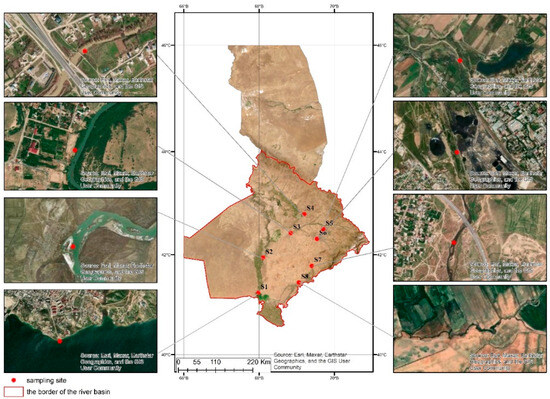
Figure 1.
Map of surface water sampling locations.

Table 1.
Locations and Geocoordinates of surface water sampling points in the Turkestan region.
2.2. Water Sampling and Analytical Methods
Field research on surface waters was conducted in August 2024. Water samples were collected from eight locations (S1–S8) using a selective sampling method. The sampling locations were chosen based on anthropogenic factors, such as industrial discharges, agricultural runoff, and domestic wastewater, which significantly affect surface water quality. The samples were taken from a depth of 15–20 cm from the water surface and stored in polyethylene bottles.
During the study, 24 chemical parameters were analyzed three times, and their average values were calculated. The samples were analyzed at the certified “Structural and Biochemical Materials” engineering testing laboratory in Shymkent. The quantitative and qualitative analysis of microelements in water samples was performed using the X-ray fluorescence energy-dispersive microanalysis (XRF-EDMA) method. The analysis was conducted with the Spectroscan MAX GF—2E X-ray spectrometer(Russia, St. Petersburg.).
This method ensures high precision and reproducibility while determining the atomic composition of samples. The XRF-EDMA technique is based on the principles of spectral analysis, studying the absorption or emission of X-rays by elements. The research was carried out under standardized laboratory conditions: temperature: 20 °C; humidity: 78%; atmospheric pressure: 716 mmHg.
The samples were prepared while preserving their physicochemical properties. To minimize deviations in the data and ensure analysis accuracy, all apparatus and containers were washed with a 10% HCl solution and rinsed with double-deionized water. When filtration was applied, samples were processed using a 0.45 µm membrane filter. If no filtration was conducted, the samples were analyzed directly to determine the total concentration.
Chemical solutions were prepared using Merck-GR grade reagents. For proper calibration of the instrument, stock solutions of each heavy metal were used to prepare calibration standards. Each sample was analyzed in triplicate, and after every three measurements, instrument deviations were checked.
The analysis was conducted using the Spectroscan GF spectrometer (St. Petersburg, Russia), capable of detecting a wide range of elements from light (Mg) to heavy (U). Calibration was performed in compliance with international standards: limit of detection (LOD): 1–20 ppm; limit of quantification (LOQ): 1–20 ppm. To accurately measure 0.001 mg/L levels of Co and Cd, specific calibration and standardization procedures were implemented. Instrument responses were monitored during each measurement to ensure the reliability of the results.
The accuracy and reproducibility of the results were ensured through the use of certified reference standards and compliance with ISO 17025 standards[*]. These measures enhanced the reliability and scientific validity of the analysis results. The concentration of sulfates (SO42−) in water samples was determined using the spectrophotometric method. This method is based on the quantitative measurement of sulfate concentrations through spectrophotometric analysis in the presence of specific reagents. To ensure the accuracy of the method, calibration was performed using standard solutions.
2.3. Variational-Statistical Analysis
First, the chemical parameters of the surface water samples collected from the Turkestan region were processed using variational-statistical analysis with MS Excel 2016. The following variational-statistical indicators were used during data processing. Each variational-statistical indicator has its own specific formula [49,50]. Below are their formulas (1):
Mean ± standard error (X ± Sx):
where
X—mean value;
σ—standard deviation;
n—number of observations.
Limit rate (lim): This indicator represents the range between the highest and lowest values (2):
Difference of limits (p): This is also used to determine the difference between the limits (3):
Standard deviation (σ): The standard deviation describes how far the data points are from the mean (4):
where
—each observation;
X—mean value;
n—number of observations.
Coefficient of variation (CV%): The coefficient of variation indicates the level of dispersion in the data (5):
where
σ—standard deviation;
X—mean value.
Principal component analysis (PCA): The principal component analysis (PCA) method was used to reduce the dimensionality of the data and identify the primary sources of variability. The method consists of the following steps:
Data standardization: To enable the comparison of variables with different units and ranges, the data were standardized using the z-score (6):
where
—the i-th observation value of the j-th variable;
—the mean value of the variable;
—the standard deviation.
Constructing the correlation matrix: To analyze the relationships between standardized variables, the correlation matrix (R) was calculated (7):
where
Z—standardized data matrix,
n—number of observations..
Eigen decomposition: Eigenvalues () and eigenvectors (v) were derived from the correlation matrix using the following Equation (8):
The eigenvalues represent the variance explained by each principal component, while the eigenvectors define the directions of these components.
Projection of data onto principal components: The standardized data were projected onto the eigenvector space to compute the principal components (9):
where PC is the matrix of principal components, and V is the matrix of eigenvectors.
PC = ZV
Explained variance: The contribution of each principal component to the total variance was calculated as follows (10):
where is the eigenvalue of the i–th principal component.
The study employed variational-statistical analysis and principal component analysis (PCA) to examine the physicochemical parameters of surface waters, including potential sources of heavy metals. Initial statistical parameters (mean, minimum, and maximum values) were calculated using MS Excel 2016. Subsequently, data analysis was performed in Python, utilizing libraries such as NumPy, Pandas, Matplotlib, and Seaborn for efficient processing and visualization.
PCA Method and Its Features
PCA identifies correlations among variables and determines their contribution to the principal components. Widely used in hydrological studies, this method reduces dataset dimensionality while retaining significant information. Only components with eigenvalues greater than 1 were considered. The Kaiser varimax rotation method was applied to clarify the contribution of components to variance and identify the primary sources of parameter variation.
Explanation of Principal Components:
PC1 (Principal component 1): Explains the largest portion of variance in the data and represents the most significant variation.
PC2 (Principal component 2): Explains the remaining variance and is orthogonal (uncorrelated) to PC1.
The values of the sampling sites reflect their direction and magnitude of influence on the components:
Positive values indicate a strong association with the component, contributing to overall variation.
Negative values indicate a reverse effect, reducing variation.
These steps facilitated the identification of the most influential components, a deeper understanding of relationships among variables, and effective dimensionality reduction. The results provide a crucial scientific basis for identifying key factors influencing surface water quality.
2.4. Water Quality Analysis
2.4.1. Overall Pollution Index (OIP)
The overall pollution index (OIP) is an important indicator for the comprehensive assessment of water resource quality. This index determines the quality of water by comparing various parameters within the water and allows for the safe use of water resources.
The OIP is calculated by determining the ratio between the actual value and the standard value of each parameter. Water quality is assessed in accordance with the water resource evaluation system in Kazakhstan (Table 2) [51]. The calculation is carried out using formula (11), with the pollution index for each parameter determined based on the average value.
Table 2.
General structure of the water quality assessment system in Kazakhstan.
The OIP characterizes the overall condition of water quality and plays a crucial role in ecological monitoring and the development of strategies for improving water quality [52].
Formula for calculating the OIP:
where
OIP—overall pollution index;
n—number of parameters considered;
—pollution index for the i-th parameter.
The pollution index for each parameter is determined using the following formula (12):
where
—measured value of the parameter;
—standard allowable value of the parameter (MAC).
This ratio determines how much each pollutant affects the water quality.
OIP Interpretation:
OIP ≤ 1.9—very clean water (C1 Class). The quality of the water source is excellent, meeting ecological and sanitary standards.
1.9 < OIP ≤ 3.9—satisfactory quality (C2 Class). The quality of the water resources is generally acceptable, but some pollutants may be present in small amounts.
3.9 < OIP ≤ 7.9—moderate pollution (C3 Class). The water resources are moderately polluted, affecting ecological stability.
7.9 < OIP ≤ 15.9—significant pollution (C4 Class). The water quality is considerably degraded, potentially leading to ecological hazards.
OIP > 15.9—highly polluted (C5 Class). The water resources do not meet ecological and sanitary standards and may pose significant risks to human health and the environment.
2.4.2. Nemerov Pollution Index (NPI)
The Nemerov pollution index (NPI) [53] is one of the important methods for assessing water quality. The NPI allows for determining the overall pollution level by calculating various water indicators and comparing them with standards. This method quantitatively describes the environmental quality, making it an effective tool in ecological monitoring and water quality assessment.
To calculate the NPI, the following formula is used for each indicator (13):
where
— the actual value of each chemical parameter in your water sample (e.g., aluminum, calcium, etc.).
— the maximum allowable concentration (MAC) of the parameter, i.e., the maximum permissible concentration.
In other words, for each parameter, the actual concentration (MAC) is divided by the maximum allowable concentration to determine how much the parameter exceeds the permissible concentration.
Interpretation of NPI values:
NPI < 1—The parameter does not exceed the allowable limit. This indicates that the water quality is good and there is no pollution.
NPI = 1—The parameter is at the allowable concentration level. This parameter is within the safe limit, but it is approaching the maximum permissible concentration.
NPI > 1—The parameter exceeds the maximum permissible concentration. This indicates that the parameter negatively affects the water quality, showing a high pollution level. The higher the NPI value, the stronger the water pollution.
2.4.3. Heavy Metal Pollution Index (HPI)
The heavy metal pollution index (HPI) is a quantitative indicator used to assess the overall pollution level of heavy metals in water. The HPI determines the contribution of each chemical parameter to water quality and was first proposed in the literature by [54].
HPI allows for studying the cumulative effect of heavy metals and determining their impact on water quality. The method evaluates the toxicity and significance of heavy metals using a weighted arithmetic mean, considering their effects on human health and river ecosystems. When calculating HPI, all analyzed metals are considered, and their compliance with the maximum allowable concentration (MAC) standards is assessed.
The formula for calculating HPI is as follows (14):
In this equation represents the weight assigned to each heavy metal, and refers to the sub-index for that heavy metal. The value of is calculated using the following Equation (15):
In this context, k is the proportionality constant (typically assumed to be k = 1k = 1k = 1), and represents the allowable standard value for the heavy metal. The variable ranges between 0 and 1. The sub-index is calculated using the following Equation (16):
In this equation, represents the value obtained through laboratory analysis, represents the ideal value, and represents the standard value for that heavy metal.
Interpretation Scale for HPI Values:
HPI < 50—safe and clean water: The concentration of heavy metals complies with ecological and sanitary standards. Such water is considered safe for ecosystems and human health.
50 ≤ HPI < 100—moderately polluted water: At this level, the concentration of heavy metals is close to the allowable limits but still acceptable. However, prolonged use may have an impact on ecosystems and health.
HPI ≥ 100—highly polluted water: The water is significantly polluted, and the concentration of heavy metals is far above the allowable limits. Such water is harmful to ecosystems and poses a significant health risk, so its use should be restricted or completely prohibited.
2.5. Land Use and Land Cover (LULC) Classification
The land use/land cover (LULC) classification for the Turkestan region is an effective method for analyzing the landscape features of the region using thematic information derived from satellite data [55]. The global land cover and land use change dataset from 2000 to 2020, obtained from the Landsat archive, was used [56]. The data obtained through LULC contribute to the effective management of land resources and land use planning, as they allow for a broad-scale assessment of land use types [57].
3. Results and Discussion
3.1. Physicochemical Indicators of Surface Waters in the Turkestan Region
Table 3 provides a variational-statistical analysis of the surface water quality analysis. Based on the variational-statistical indicators, PCA (principal component analysis) was conducted to effectively evaluate the variability of heavy metal concentrations in the water samples. For PCA analysis, a correlation matrix was used because the variables were measured in different units. This approach allowed for effective evaluation of relationships between variables by standardizing them. Table 4 shows that PCA identified two principal components, explaining 64.8% of the total variability in the dataset. Table 5 presents the factor loadings for each parameter, describing their relationships with the two principal components. These factor loadings represent the contribution of each parameter to the two main components. Positive or negative values indicate the direction of the relationship between the parameters and the components.
Table 3.
Variational-statistical data of physicochemical indicators of surface waters in the Turkestan region (2024).
Table 4.
Statistical indicators of surface water samples based on principal components (PC1 and PC2).
Table 5.
Factor loadings of parameters in principal component analysis (PCA) for surface water quality.
The climate of the Turkestan region is distinctly continental, with very hot summers and relatively cool winters. In July, temperatures exceed 40 °C, and in winter, the average temperature drops between −5 °C and −10 °C. The water temperature in the summer months ranges from 22 °C to 30 °C [47], which affects biological activity.
In the temperate climatic conditions, especially in summer, water parameters such as acidity (pH), hardness, and dissolved oxygen remain mostly stable. Seasonal fluctuations are relatively small, but the high summer temperatures affect plants and animals.
The Turkestan region is a very arid area, with annual precipitation ranging from 150 to 300 mm, which is a critical factor for water resources and landscape stability.
The PCA results identified two principal components of the water samples: PC1 and PC2. Each component’s loadings describe the major variations and changes in water composition.
PC1 component: PC1 defines the mineral composition of the water. The main loadings of this component are closely associated with parameters such as total hardness, total dissolved solids (TDSs), and mineral elements like Al, Ca, and Mg. For example, total hardness (−0.35) and TDS (−0.32) indicate a high level of water mineralization. The loadings for Ca and Mg are −0.33 and −0.35, respectively, confirming that these are the primary elements contributing to water hardness.
PC2 component: PC2 reflects the presence of heavy metals and pollutants, such as Ti, Fe, Pb, and Cu. The loadings for this component are as follows: Fe has a value of 0.59, indicating a high concentration of iron in the water. The loadings for Pb and Cu are 5.57 and 2.44, respectively, which clearly signify contamination with heavy metals.
Description of water samples: Based on the PCA results, the water samples from the Turkestan region can be clustered according to the values of the two principal components as follows: S1: (PC1 = −1.46, PC2 = −1.82)—ecologically clean water with low concentrations of mineral elements. S2: (PC1 = −0.99, PC2 = −0.20)—moderate levels of mineral elements, minimal heavy metals. S3: (PC1 = −0.85, PC2 = 0.08)—potential presence of heavy metals and pollutants at low levels. S4: (PC1 = 0.77, PC2 = 1.51)—high levels of mineral and metallic pollutants. S5: (PC1 = 0.89, PC2 = −0.93)—elevated mineral content, low levels of heavy metals. S6: (PC1 = 0.30, PC2 = 0.38)—low levels of both mineral content and heavy metals. S7: (PC1 = −0.38, PC2 = 2.32)—high concentration of heavy metals. S8: (PC1 = 3.50, PC2 = −1.18)—high levels of both mineral and metallic pollutants.
Coefficient of variation (CV%) and standard deviation: The Al parameter shows a CV% of 137.99%, indicating significant variability in its concentration. The pH parameter has a CV% of 1.71%, reflecting its stability. Parameters such as total hardness (σ = 3.08) and TDS (σ = 382.40) exhibit high standard deviations, suggesting notable variation.
Insights and implications: The PCA method provides a deeper understanding of the chemical composition of water samples from the Turkestan region. Variations in mineral and metallic pollutants highlight the importance of environmental monitoring. Each water source has distinct chemical characteristics, requiring targeted measures to improve water quality [58,59]. This study identifies changes in contamination and mineral composition in the water sources of the Turkestan region, offering valuable data for ecological monitoring [60]. The elevated levels of heavy metals (e.g., Fe, Pb) necessitate appropriate measures to improve water quality [61,62,63]. Such actions contribute to maintaining ecosystem stability and the sustainable management of regional water resources.
3.2. Water Quality Analysis
3.2.1. Water Quality Analysis Through the Overall Pollution Index (OIP)
Water quality evaluation was conducted through the overall pollution index (OIP). This index includes the analysis of 24 physicochemical parameters: total hardness, pH, total dissolved solids, electrical conductivity, total salt content, Al, As, B, Ca, Cd, Co, Cr, Ti, Fe, Pb, Cu, Mg, K, Mn, Na, Ni, Zn, SO42−, and C6H5OH. These parameters are based on the analyses conducted at the sampling sites in the Turkestan region.
These parameters were selected as key factors affecting water quality and assist in determining the suitability of the chemical composition and physical properties for ecological safety and industrial use. The OIP is calculated by considering the maximum allowable concentrations (MAC) of substances in water and their potential impacts on landscapes (Figure 2, Table 6).
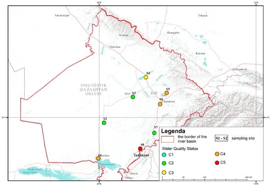
Figure 2.
Map of the overall pollution index (OPI) values for surface waters in the Turkestan region.
Table 6.
Overall pollution index (OPI) values for surface waters in the Turkestan region.
The results of the water quality analysis of the main rivers in the Turkestan region showed that the quality of surface waters is directly dependent on both natural processes and anthropogenic factors. The water quality at the S1–S8 sampling points is characterized by various indicators. The study identified differences in the chemical composition, physical, and microbiological indicators of the water, as well as the level of pollution at each sampling point.
The water quality at the sampling sites S2 (OPI = 0.56), S3 (OPI = 0.43), and S7 (OPI = 0.73) is at a satisfactory level. The good water quality at these points is primarily due to the absence of Al, with its concentration being 0.00 mg/L. The absence of Al prevents the negative impact of heavy metals on landscapes, contributing to the higher water quality. Additionally, high levels of total hardness were recorded in these rivers, indicating a high degree of mineralization of the water. However, the abundance of Ca and Mg2+ ions can lead to equipment wear and increased maintenance costs [64].
The high level of electrical conductivity indicates the presence of a large number of dissolved ions and salts in the water, which can lead to soil salinization. For example, the sodium concentration at the S7 sampling point is 180.05 mg/L, which increases the risk of soil salinization [65]. Although the water quality is rated as satisfactory according to the OIP indicators, the high levels of Ca, Mg2+, Na+, and Cl− ions could negatively impact the quality of water resources in the long term.
At the S4 sampling point (OIP = 1.27), the water quality is considered to be at a moderate pollution level. The concentration of Al is 2.42 mg/L, which is the main cause of water contamination. The high level of aluminum contributes to the increase in the OIP value. The presence of high levels of Al in the water ecosystem negatively affects the stability of landscapes [66,67,68,69]. The low electrical conductivity value (555 µS/cm) indicates that the water contains fewer dissolved ions and salts, which is an important factor for agriculture.
At the S1 (OIP = 3.1), S5 (OIP = 2.38), and S6 (OIP = 3.68) sampling points, the water quality indicates a high level of pollution, confirming their classification as Class 4. The concentration of Al is 6.68 mg/L at S1, 5.47 mg/L at S5, and 6.15 mg/L at S6. Total hardness is 10.64 mg-equiv/L at S1, 7.36 mg-equiv/L at S5, and 8.07 mg-equiv/L at S6, with electrical conductivity recorded as 1635 µS/cm, 617 µS/cm, and 825 µS/cm, respectively. These values indicate a high level of mineralization [70,71].
At S1, the Na+ concentration is recorded at 146.35 mg/L, leading to an increase in salinity. The SO42− concentration is 639 mg/L at S1, 92.2 mg/L at S5, and 153 mg/L at S6, which are indicators of mineralization.
At the S8 (OIP = 12.14) sampling point, the water quality shows an extreme level of pollution. The Al concentration (22.38 mg/L) is several times higher than the maximum allowable concentration (MAC), which has a toxic effect on the water ecosystem and plants.
The high level of total hardness (10.92 mg-equiv/L) indicates a significantly high degree of mineralization in the water. The elevated Na+ concentration (157.42 mg/L) presents a salinity issue.
The Cd concentration (0.001 mg/L) and Co concentration (0.001 mg/L) pose a threat to the water ecosystem, while the Cr concentration (0.003 mg/L) could negatively affect water quality. The Fe concentration (12.76 mg/L) leads to excessive algae growth and a reduction in oxygen levels [71].
The water quality indicators at the sampling points in the Turkestan region reflect the impact of both geological and anthropogenic factors. High concentrations of Al and Fe are the result of natural erosion and industrial waste. The study highlights the need for proper fertilizer use in agriculture, control of industrial pollution, and enhanced anti-erosion measures [72].
3.2.2. Analysis Using the Nemerov Pollution Index (NPI)
The pollution index (NPI) values for the sampling points show significant variation in the pollution levels of different chemical elements (Table 7). The results for the S8 sampling point indicate very poor water quality, while other points show moderate levels of pollution. The concentration of Al exceeded the threshold at all sampling points, with particularly high levels observed at S1 (NPI = 26) and S8 (NPI = 45). Such high concentrations of Al are harmful to landscapes, agriculture, and human health, presenting a significant risk for water resource use. The high levels of Al indicate a persistent pollution source, which could be due to natural erosion or anthropogenic influences [73].
Table 7.
Nemerov pollution index (NPI) values of surface waters in the Turkestan region.
The concentration of Fe was highest at the S8 sampling point (NPI = 43), indicating ecological hazards associated with the water. The Fe pollution at S5 (NPI = 8) was also notably high, exceeding the standard limits. Excessive Fe can disrupt ecological balance, alter the taste and color of the water, and negatively impact living organisms [72].
Total hardness (CaCO3) remains within the allowable limits at all sampling points (NPI < 1), indicating that the water quality is good. The pH levels are within the permissible range, meaning the water’s acid–base balance is normal. High electrical conductivity values were recorded at the S1 and S7 sampling points (NPI = 1.6 and 1.7), indicating a high degree of mineralization in the water.
The elevated levels of Al and Fe in the water significantly lower water quality and make it ecologically hazardous. At the S8 sampling point (OIP = 12.14), the water quality was found to be at an extreme level of pollution. The Al concentration (22.38 mg/L) is several times higher than the MAC, which has a toxic effect on the water ecosystem and plants.
The deterioration in water quality is associated with the high concentration of Al, while the high levels of Fe (12.76 mg/L) and total hardness (10.92 mg-equiv/L) indicate a high degree of mineralization. The concentrations of Cd (0.001 mg/L) and Co (0.001 mg/L) can harm the ecosystem, while Cr (0.003 mg/L) has carcinogenic effects.
Both NPI and OIP provide valuable information for assessing water quality, but each reflects pollution levels from different perspectives. NPI highlights the impact of specific parameters (e.g., Al, Fe) on water quality, while OIP describes the overall quality. A comparison of the two indices shows an increase in pollution levels, which helps to understand the factors influencing water quality [74]. It is crucial to take necessary actions for water resource management and to reduce pollution levels.
3.2.3. Heavy Metal Pollution Index (HPI)
The heavy metal pollution index (HPI) was calculated individually for each sampling point, allowing for a comparison of pollution loads and an assessment of water quality (Table 8). HPI reflects the cumulative effect of various heavy metals. According to the MAC (2016) standards, if the HPI value exceeds 100, the water is considered significantly polluted.
Table 8.
Heavy metal pollution index (HPI) values of the Turkistan region.
In the study, the HPI values for the S4 and S8 sampling points significantly exceeded 100, reaching 120.38 and 4253.33, respectively. These values indicate high levels of pollution with heavy metals and confirm that the water sources are ecologically and health-wise hazardous to human health [75].
The analyzed data allow for the assessment of heavy metal pollution levels at various points. The HPI indicator clearly distinguishes between high and low levels of pollution.
The S8 sampling point falls under the category of extremely dangerous pollution, with an HPI value of 4253.33, the highest value in the region. This high value is primarily due to the very high concentration of Fe (12.76 mg/L), which is 42 times above the maximum allowable concentration (MAC) level of 0.3 mg/L. Such pollution renders the water source unsuitable for ecological and agricultural purposes. Therefore, urgent measures are needed at the S8 sampling point to address pollution sources and implement water treatment.
At the S4 sampling point, the HPI value is 120.38, indicating a dangerous level of pollution. The concentration of Fe at this point is 12.76 mg/L, significantly exceeding the MAC level. While the pollution level is lower than at S8, this area is still categorized as highly polluted.
At the S1, S2, S3, and S5 sampling points, water quality is good, with HPI values below 50. These water sources are safe for both ecological and agricultural use. At these points, the concentration of heavy metals is at its lowest, which results in good water quality. However, continued monitoring is important to ensure that pollution levels remain under control [76,77].
At the S8 and S4 sampling points, extremely high levels of pollution were recorded, while S1, S2, and S5 showed moderate pollution, and S3 had the least pollution. At the most polluted points, restrictions on water use should be implemented, and measures to eliminate pollution sources need to be taken. Even in moderately polluted areas, it is important to strengthen monitoring efforts.
Principal component analysis (PCA) was conducted based on the correlation matrix for the Turkestan region. The analysis resulted in the identification of four principal components, with eigenvector values above 1, explaining 92.34% of the total variance [78]. Factor loadings above 0.5 were considered significant, and the correlation coefficients between the metals ranged from 0.87 to 1, indicating that the metals were appropriately distributed across the identified factors.
3.3. Land Use Changes and Water Quality
Changes in land use affect the stability of landscapes and directly impact the quality of water resources. The deterioration of water ecosystems poses risks to biodiversity, agricultural productivity, and public health. In the Turkestan region, landscape changes and anthropogenic factors contribute to the decline in water quality. Based on global land cover and land use change data from 2000 to 2020 obtained from the Landsat archive, the land cover classification in the Turkestan region was divided into the following categories: short vegetation, permanent tree cover, trees after degradation, seasonal water bodies, permanent snow/ice, permanent water, permanent agricultural land, and permanent structures. This map is shown in Figure 3.

Figure 3.
Land use and land cover (LULC) classification map of surface waters in the Turkestan region.
The study results showed that the expansion of agriculture and urbanization has caused significant changes in land cover. The excessive use of fertilizers in agriculture, increased construction, and the expansion of grazing lands have had negative impacts on water bodies. Soil erosion, chemical pollution, and salinization processes have contributed to the deterioration of water quality.
The overall pollution index (OIP) was used to assess water quality. Water samples were taken from eight points (S1–S8) for analysis. At the S4 sampling point, the OIP was 1.27, indicating that the water was moderately polluted (Class 3). The main cause of pollution was the Al concentration reaching 2.42 mg/L. Other indicators, such as hardness and Na levels, showed lower values and had less impact on the OIP [79,80,81].
At the S8 sampling point, the OIP reached 12.14, indicating an extremely high level of pollution (Class 5). The water contamination at this point is primarily due to the concentration of Al (22.38 mg/L), which is several times higher than the maximum allowable concentration (MAC). Additional indicators showed that total hardness was 10.92 mg-equiv/L, electrical conductivity was 1493 µS/cm, and Na concentration was 157.42 mg/L. These results confirm that the water at the S8 point is unsuitable for ecological and agricultural purposes [82].
To assess the concentration of heavy metals, the heavy metal pollution index (HPI) was used. The HPI was calculated based on the concentrations of Cd, Co, Cr, and Fe. At the S8 point, the Fe concentration reached 12.76 mg/L, which is significantly higher than the MAC (0.3 mg/L). Such a high level of Fe poses a significant threat to the water ecosystem and makes the water unsafe for use.
Other metals, such as Cd and Cr, were within permissible limits at several points, but it is important to consider their cumulative effects. The study results showed that inefficient land use negatively impacts water resources. The excessive use of fertilizers and chemicals in agriculture contributed to the increase in heavy metals and chemical indicators [83].
The expansion of construction and urbanization has increased the electrical conductivity and hardness of the water, leading to salinization issues. The increase in grazing areas has intensified soil erosion and contributed to the influx of solid waste into the water. The exceedance of these indicators from quality standards was mainly due to domestic, industrial, and agricultural runoff [84,85,86,87,88]. Table 9 shows pollutants that require attention, their sources, impacts, and management methods.
Table 9.
Natural and anthropogenic sources of pollutants, their ecological impacts, and technical solutions for mitigation [36,89,90,91,92,93].
3.4. Indirect Effects of Chemical Pollution Load in Surface Waters on Landscapes
Key water quality indicators (total hardness, Al, electrical conductivity, Na) directly affect soil fertility and vegetation cover. The increase in Al levels (S8: 22.38 mg/L) enhances soil acidity, reducing the quality of land suitable for agriculture. This accelerates soil salinization and degradation processes, increasing the risk of desertification.
The high electrical conductivity value (1493 µS/cm) indicates significant accumulation of sodium salts, which contributes to the degradation of soil structure. This negatively impacts the growth of agricultural crops and weakens ecosystem function. The S8 sampling point indicates that the ecosystem has surpassed its resilience threshold (OIP = 12.14), demonstrating that the water is unsuitable for use [94].
The accumulation of heavy metals, particularly Fe and Cd, accelerates landscape degradation. The Fe concentration at the S8 point reached 12.76 mg/L, causing eutrophication and oxygen depletion in aquatic ecosystems. Although Cd is found in low concentrations (S1, S2, S5: 0.001 mg/L), it can bioaccumulate in living organisms over time.
3.5. Water Pollution’s Impact on Local Hydrological Cycles and Landscapes
Water pollution affects local hydrological cycles and alters the chemical composition of groundwater. The pollution levels at the S4 and S8 sampling points (OIP: 1.27 and 12.14) influence river flows and groundwater levels. These changes may lead to soil swampification or desertification, particularly observed near the S6 sampling point [95].
At S2, water quality (OIP = 0.56) is normal, but long-term monitoring is necessary to prevent future increases in pollution [96,97]. The Fe concentration at S4 and S8 points (2.42–12.76 mg/L) slows down plant growth and degrades fish habitats. As a result, vegetation along riverbanks becomes sparse, forcing birds and animals to migrate.
The interconnection between water quality and landscapes is a critical factor for the stability of ecosystems in the Turkestan region. High concentrations of heavy metals and physicochemical indicators exacerbate landscape degradation and disrupt ecological balance.
Reducing water pollution through long-term ecological monitoring and implementing restoration strategies is essential to preserve the stability of natural ecosystems and enable adaptation to climate change [57].
3.6. Purification of River Water Contaminated with Heavy Metals
Purifying rivers contaminated with heavy metals is crucial for maintaining ecological balance and protecting public health. Cd, Pb, and Fe are harmful to the environment and biological organisms, causing various diseases when accumulated in the human body. The effectiveness of purification technologies depends on the level of contamination and economic costs. The primary methods used include adsorption, ion exchange, membrane filtration, and advanced oxidation processes (AOPs).
Kosar Hama Aziz et al. (2023) [98] demonstrated that biochar and zeolite effectively adsorb heavy metals such as Cd, Pb, and Cr. Similarly, Inglezakis V.J. (2003) [99] investigated the use of clinoptilolite for heavy metal removal via ion exchange; however, resin contamination posed challenges for long-term applications. Mashangwa T.D. (2016) [100] investigated the effectiveness of using egg shells as a low-cost adsorbent to remove heavy metals. Roongtanakiat and colleagues (2007) [101] determined the effectiveness of vetiver grass in accumulating Pb, Cd, and Cr. Kidd and Monterroso (2005) [102] studied the hyperaccumulation properties of this plant. Ingole and Bhole (2003) [103] demonstrated the Pb and Cd absorption capabilities of water hyacinth.
Analyzing these studies, we focus on biological methods for heavy metal purification and propose phytoremediation. This method offers an ecologically safe and economically efficient solution by using plants with high effectiveness in accumulating heavy metals.
Phytoremediation is a method of purifying water using plants capable of accumulating heavy metals. Plants such as Populus spp., Tamarix spp., Phragmites australis, Carex spp., Medicago sativa, Lupinus spp., Typha latifolia, and Salix spp. are recommended for use in the riverbanks of the Turkestan region [104]. These plants absorb metals like Fe, Cd, and Zn, and help protect the banks from erosion (Table 10). The use of the rhizofiltration method, where plant roots are directed towards wastewater, can enhance the process of metal absorption. Aquatic plants—whether emergent, floating, or submerged—have unique roots and shoots that increase their ability to absorb substances from their growth environment, helping to reduce the concentration of pollutants in targeted water bodies.
Table 10.
Accumulation capacity of heavy metals by different aquatic plants [105,106,107].
Phytoremediation involves physical, chemical, and biological processes. This method helps reduce heavy metal levels in water ecosystems and restores natural balance.
The phytoremediation process relies on several key mechanisms:
- Accumulation of pollutants (phytoextraction and rhizofiltration);
- Immobilization of pollutants (phytostabilization);
- Biodegradation (rhizodegradation and phytodegradation);
- Dissipation (phytovolatilization).
These mechanisms help limit the spread of pollutants in the environment, promote their degradation, or transform them into a more stable form.
The combination of mechanisms used with macrophytes for the removal and degradation of pollutants primarily depends on the plant species, the properties of the pollutant, and the location of the pollution within the water body (water column, lake, or sediment at the bottom of flowing water).
To assess the potential for phytoremediation, it is necessary to calculate the bioconcentration factor (BCF) by comparing the concentration of the pollutant in the plant and the water body. This coefficient is expressed in L/kg and describes the plant’s ability to absorb the pollutant. The phytoremediation mechanisms commonly found in aquatic plants are summarized in Table 11 [108,109,110,111].
Table 11.
Mechanisms used in phytoremediation with aquatic plants and pollutants [112,113,114,115,116,117].
By applying this method, the potential for comprehensive water purification and ensuring the stability of river ecosystems increases. This approach will not only improve the water quality of the rivers in the Turkestan region but also help maintain ecological balance and allow for the efficient use of water resources. Recycling plant biomass for bioenergy production or using it as fertilizer will enhance economic efficiency. Additionally, utilizing plant species adapted to the local climate will contribute to maintaining the ecosystem’s stability.
In conclusion, the following actions are recommended for the phytoremediation of water resources in the Turkestan region:
- Continuous water quality monitoring: Use sensors to monitor the dynamics of heavy metals.
- Adaptation of local plant species: Utilize plants adapted to the local climatic conditions.
- Recycling plant biomass: Use the biomass obtained after purification as a source of bioenergy.
- Conduct additional scientific research: Continue research to find effective solutions adapted to different ecosystems.
- These recommendations will allow for the ecological, safe, and sustainable restoration of the water resources in the Turkestan region.
3.7. Limitations of This Study
Currently, there are several limitations in the methods used to assess water quality, which complicates the practical application of research results. Firstly, assessment methods often focus on individual indicators and do not employ a comprehensive approach. Researchers typically focus on changes in pollutant levels and the physical-chemical properties of water but fail to provide a holistic evaluation of the overall ecosystem. This approach reduces the effectiveness of project management and remediation measures and hinders the development of accurate solutions. The lack of real-world examples of these methods also limits the applicability of the research. In terms of this study’s limitations, there is a clear need to gather additional data on organic pollutants and incorporate them into various index systems. This would ensure the comprehensiveness and integrity of the research methods, thereby enhancing the effectiveness of environmental monitoring. Furthermore, the failure to account for the accumulation characteristics of heavy metals in ecosystems remains a critical issue. Specifically, the interactions of heavy metals with biological systems, particularly tissues, and their ecotoxicological effects are still underexplored. These interactions may complicate their impact, necessitating further investigation and analysis. Thus, enhancing the data on both organic and inorganic pollutants and exploring their connections with ecological systems is essential for developing scientifically sound solutions and effective remediation measures. Additionally, the failure to account for the accumulation characteristics of heavy metals in ecosystems remains a major issue. For instance, some metals accumulate in biological tissues and pose a threat to ecosystems and human health. However, more detailed analysis is needed regarding the interactions of metals with each other and other chemicals, as their effects may depend on their interactions. These findings highlight the need to acknowledge the shortcomings in heavy metal monitoring and remediation techniques and emphasize the importance of employing a multidimensional approach to address pollution problems [57,117,118].
3.8. Future Research Needs
Future studies should focus on fully assessing temporal changes by collecting samples across different seasons. This will provide a deeper understanding of the seasonal dynamics of water quality and its impact on landscapes.
Including additional rivers and water sources in the study will help better understand the spatial distribution patterns of water quality. It will also contribute to identifying ecologically vulnerable areas in the region.
Future research should also incorporate the analysis of BOD, nitrates, and phosphates, as they are crucial for evaluating the health of water ecosystems. These data will enhance the understanding of the ecological functions of water bodies.
The use of remote sensing, GIS technologies, and climate models will help determine the connections between water quality, land use, and climate change. This approach will enable a more detailed analysis of the development patterns of landscapes.
Assessing the impact of changes in water quality on biodiversity and ecosystem services will be an important direction for future research. Long-term biological monitoring will help define the irreversible thresholds of changes in ecosystems.
Establishing a sustainable monitoring system will allow for continuous tracking of water quality and landscape changes over time. This will contribute to the effective management of natural resources in the region and the development of scientifically based policies.
Considering these limitations and following the proposed future research directions will deepen the understanding of the interconnection between water quality and landscapes in the Turkestan region and will contribute to the sustainable development of the region.
4. Conclusions
The comprehensive hydrochemical analysis of the surface waters in the Turkestan region has revealed the deterioration of the water resources’ ecological status under the influence of anthropogenic factors. The assessment based on the overall pollution index (OIP), Nemerov pollution index (NPI), and heavy metal pollution index (HPI) indicated that the concentrations of aluminum (Al) and iron (Fe) significantly exceeded the permissible limits. At sampling point S8, the OIP value reached 12.14, confirming an extreme level of pollution (Al—22.38 mg/L, Fe—12.76 mg/L), rendering the water unsuitable for ecological and economic purposes.
The spatial distribution of heavy metals demonstrated that at sampling points S1, S5, and S6, Al concentrations ranged between 5.47 and 6.68 mg/L, contributing to landscape degradation and disrupting ecosystem balance. Additionally, elevated concentrations of sodium (Na), magnesium (Mg), and sulfates (SO42−) increased water mineralization and accelerated secondary salinization processes, adversely affecting agricultural activities and reducing the efficiency of irrigation systems.
The HPI and NPI indices confirmed that the level of heavy metal pollution in the studied water bodies poses a significant environmental risk. Analysis of water samples revealed a high potential for long-term accumulation of Fe, Cd, and Pb in biotic environments. Furthermore, anthropogenic activities led to increased NO3− and PO43− levels, intensifying eutrophication processes. The expansion of urbanization and construction activities exacerbated soil erosion and land degradation.
The study results indicate that heavy metal contamination in the surface waters of the Turkestan region severely impacts water quality and poses a considerable threat to ecosystem stability. To mitigate pollution and improve water quality, plant-based purification technologies (phytoremediation) are proposed as an effective solution. These findings provide a scientific basis for decision-making in resource management and environmental protection, ensuring the long-term sustainability of natural ecosystems.
Author Contributions
Conceptualization—D.A. and Z.O.; methodology—N.R. and Z.K.; software—N.R. and Z.K.; validation—D.A., S.S., Z.I. and R.A.; formal analysis—S.S. and R.A.; investigation—D.A., R.K. and Z.S. (Zhadra Shingisbayeva); resources—Z.O. and M.A.; data curation—Z.I. and Z.S. (Zhadra Shingisbayeva); writing—original draft preparation—D.A. and Z.S. (Zhadra Shingisbayeva); writing—review and editing—Z.O., N.R., R.A. and Z.S. (Zhamila Sikhynbayeva); visualization—S.S. and Z.S. (Zhamila Sikhynbayeva). All authors have read and agreed to the published version of the manuscript.
Funding
This research received no external funding.
Data Availability Statement
The data used in this study are contained within the article. Additional data are available upon request from the corresponding author.
Acknowledgments
The samples were analyzed at the certified “Structural and Biochemical Materials” engineering testing laboratory at M. Auezov South Kazakhstan State University in Shymkent.
Conflicts of Interest
The authors declare no conflicts of interest. The funders had no role in the design of the study; in the collection, analyses, or interpretation of data; in the writing of the manuscript; or in the decision to publish the results.
References
- Bunn, S.E.; Davies, P.M.; Mosisch, T.D. Ecosystem measures of river health and their response to riparian and catchment degradation. Freshw. Biol. 1999, 41, 333–345. [Google Scholar] [CrossRef]
- Newson, M. Understanding ‘hot-spot’ problems in catchments: The need for scale-sensitive measures and mechanisms to secure effective solutions for river management and conservation. Aquat. Conserv. Mar. Freshw. Ecosyst. 2010, 20, S62–S72. [Google Scholar] [CrossRef]
- Guermazi, E.; Milano, M.; Reynard, E.; Zairi, M. Impact of climate change and anthropogenic pressure on the groundwater resources in arid environment. Mitig. Adapt. Strat. Glob. Chang. 2018, 24, 73–92. [Google Scholar] [CrossRef]
- Bracken, L.J.; Croke, J. The concept of hydrological connectivity and its contribution to understanding runoff-dominated geomorphic systems. Hydrol. Process. 2007, 21, 1749–1763. [Google Scholar] [CrossRef]
- Fernandes, A.C.P.; de Oliveira Martins, L.M.; Pacheco, F.A.L.; Fernandes, L.F.S. The consequences for stream water quality of long-term changes in landscape patterns: Implications for land use management and policies. Land Use Policy 2021, 109, 105679. [Google Scholar] [CrossRef]
- Ba, W.; Du, P.; Liu, T.; Bao, A.; Chen, X.; Liu, J.; Qin, C. Impacts of climate change and agricultural activities on water quality in the Lower Kaidu River Basin, China. J. Geogr. Sci. 2020, 30, 164–176. [Google Scholar] [CrossRef]
- Alamri, D.A.; Al-Solaimani, S.G.; Abohassan, R.A.; Rinklebe, J.; Shaheen, S.M. Assessment of water contamination by potentially toxic elements in mangrove lagoons of the Red Sea, Saudi Arabia. Environ. Geochem. Health 2021, 43, 4819–4830. [Google Scholar] [CrossRef] [PubMed]
- Quan, J.; Xu, Y.; Ma, T.; Wilson, J.P.; Zhao, N.; Ni, Y. Improving surface water quality of the Yellow River Basin due to anthropogenic changes. Sci. Total Environ. 2022, 836, 155607. [Google Scholar] [CrossRef] [PubMed]
- Hussein, A. Impacts of land use and land cover change on vegetation diversity of tropical highland in Ethiopia. Appl. Environ. Soil Sci. 2023, 2023, 1–11. [Google Scholar] [CrossRef]
- Pandey, P.C.; Koutsias, N.; Petropoulos, G.P.; Srivastava, P.K.; Ben Dor, E. Land use/land cover in view of earth observation: Data sources, input dimensions, and classifiers—A review of the state of the art. Geocarto Int. 2021, 36, 957–988. [Google Scholar] [CrossRef]
- Chaemiso, S.E.; Kartha, S.A.; Pingale, S.M. Effect of land use/land cover changes on surface water availability in the Omo Gibe basin, Ethiopia. Hydrol. Sci. J. 2021, 66, 1936–1962. [Google Scholar] [CrossRef]
- Emenike, P.C.; Tenebe, I.T.; Neris, J.B.; Omole, D.O.; Afolayan, O.; Okeke, C.U.; Emenike, I.K. An integrated assessment of land-use change impact, seasonal variation of pollution indices and human health risk of selected toxic elements in sediments of River Atuwara, Nigeria. Environ. Pollut. 2020, 265, 114795. [Google Scholar] [CrossRef] [PubMed]
- Phanmala, K.; Lai, Y.; Xiao, K. Impact of land use change on the water environment of a key marsh area in Vientiane Capital, Laos. Water 2023, 15, 4302. [Google Scholar] [CrossRef]
- Qiu, Z.; Kennen, J.G.; Giri, S.; Walter, T.; Kang, Y.; Zhang, Z. Reassessing the relationship between landscape alteration and aquatic ecosystem degradation from a hydrologically sensitive area perspective. Sci. Total Environ. 2019, 650, 2850–2862. [Google Scholar] [CrossRef]
- Bhat, S.U.; Khanday, S.A.; Islam, S.T.; Sabha, I. Understanding the spatiotemporal pollution dynamics of highly fragile montane watersheds of Kashmir Himalaya, India. Environ. Pollut. 2021, 286, 117335. [Google Scholar] [CrossRef] [PubMed]
- Mello, K.D.; Taniwaki, R.H.; Paula, F.R.D.; Valente, R.A.; Randhir, T.O.; Macedo, D.R.; Leal, C.G.; Hughes, R.M. Multiscale land use impacts on water quality: Assessment, planning, and future perspectives in Brazil. J. Environ. Manag. 2020, 270, 110879. [Google Scholar] [CrossRef] [PubMed]
- Ma, B.; Wu, C.; Jia, X.; Zhang, Y.; Zhou, Z. Predicting water quality using partial least squares regression of land use and morphology (Danjiangkou Reservoir, China). J. Hydrol. 2023, 624, 129828. [Google Scholar] [CrossRef]
- Mitchell, M.G.E.; Bennett, E.M.; Gonzalez, A. Linking Landscape Connectivity and Ecosystem Service Provision: Current Knowledge and Research Gaps. Ecosystems 2013, 16, 894–908. [Google Scholar] [CrossRef]
- Zhang, J.; Li, S.; Dong, R.; Jiang, C.; Ni, M. Influences of land use metrics at multi-spatial scales on seasonal water quality: A case study of river systems in the Three Gorges Reservoir Area, China. J. Clean. Prod. 2019, 206, 76–85. [Google Scholar] [CrossRef]
- Abazeri, M. Women of the Sun: Mediating Co-Production in Iranian Agrarian Systems. Ph.D. Thesis, University of Miami, Coral Gables, FL, USA, 2023. Available online: https://scholarship.miami.edu/esploro/outputs/991031786017502976 (accessed on 1 December 2024).
- Mrabet, R. Sustainable agriculture for food and nutritional security. In Sustainable Agriculture and the Environment; Mrabet, R., Ed.; Elsevier: Amsterdam, The Netherlands, 2023; pp. 25–90. [Google Scholar]
- Nwachukwu, B.C. Microbial Diversity, Community Structure and Functional Characteristics of Sunflower Rhizospheric Soil. Ph.D. Thesis, North-West University, Potchefstroom, South Africa, 2023. Available online: https://repository.nwu.ac.za/dissertations/nwachukwu-2023 (accessed on 1 December 2024).
- Ding, J.; Jiang, Y.; Liu, Q.; Hou, Z.; Liao, J.; Fu, L.; Peng, Q. Influences of the land use pattern on water quality in low-order streams of the Dongjiang River basin, China: A multi-scale analysis. Sci. Total Environ. 2016, 551–552, 205–216. [Google Scholar] [CrossRef]
- Barroso, G.R.; Pinto, C.C.; Gomes, L.N.L.; Oliveira, S.C. Assessment of water quality based on statistical analysis of physical chemical, biomonitoring and land use data: Manso River supply reservoir. Sci. Total Environ. 2024, 912, 169554. [Google Scholar] [CrossRef]
- Chattopadhayay, R.; Ghosh, A.K. Performance appraisal based on a forced distribution system: Its drawbacks and remedies. Int. J. Product. Perform. Manag. 2012, 61, 881–896. [Google Scholar] [CrossRef]
- Uddin, M.G.; Nash, S.; Olbert, A.I. A review of water quality index models and their use for assessing surface water quality. Ecol. Indic. 2021, 122, 107218. [Google Scholar] [CrossRef]
- Dawood, A.S. Using of Nemerow’s Pollution Index (NPI) for water quality assessment of some Basrah Marshes, South of Iraq. J. Babylon Univ. Pure Appl. Sci. 2017, 25, 1708–1720. [Google Scholar]
- Subagiyo, L.; Nuryadin, A.; Sulaeman, N.F.; Widyastuti, R. Water quality status of Kalimantan water bodies based on the pollution index. Pollut. Res. 2019, 38, 536–543. [Google Scholar]
- Hu, B.; Shao, S.; Ni, H.; Fu, Z.; Hu, L.; Zhou, Y.; Min, X.; She, S.; Chen, S.; Huang, M.; et al. Current status, spatial features, health risks, and potential driving factors of soil heavy metal pollution in China at province level. Environ. Pollut. 2020, 266, 114961. [Google Scholar] [CrossRef]
- Mitra, S.; Chakraborty, A.J.; Tareq, A.M.; Bin Emran, T.; Nainu, F.; Khusro, A.; Idris, A.M.; Khandaker, M.U.; Osman, H.; Alhumaydhi, F.A.; et al. Impact of heavy metals on the environment and human health: Novel therapeutic insights to counter the toxicity. J. King Saud Univ. Sci. 2022, 34, 101865. [Google Scholar] [CrossRef]
- Munir, N.; Jahangeer, M.; Bouyahya, A.; El Omari, N.; Ghchime, R.; Balahbib, A.; Aboulaghras, S.; Mahmood, Z.; Akram, M.; Shah, S.M.A.; et al. Heavy metal contamination of natural foods is a serious health issue: A review. Sustainability 2021, 14, 161. [Google Scholar] [CrossRef]
- Sharma, R.; Agrawal, P.R.; Kumar, R.; Gupta, G. Current scenario of heavy metal contamination in water. In Contaminants in Water; Elsevier: Amsterdam, The Netherlands, 2021; pp. 49–64. [Google Scholar]
- Zaynab, M.; Al-Yahyai, R.; Ameen, A.; Sharif, Y.; Ali, L.; Fatima, M.; Khan, K.A.; Li, S. Health and environmental effects of heavy metals. J. King Saud Univ. Sci. 2022, 34, 101653. [Google Scholar] [CrossRef]
- Ali, M.M.; Hossain, D.; Al-Imran, A.; Khan, M.S.; Begum, M.; Osman, M.H. Environmental pollution with heavy metals: A public health concern. In Heavy Metals—Their Environmental Impacts and Mitigation; IntechOpen: London, UK, 2021; pp. 771–783. [Google Scholar]
- Authman, M.M.; Zaki, M.S.; Khallaf, E.A.; Abbas, H.H. Use of fish as bio-indicator of the effects of heavy metals pollution. J. Aquac. Res. Dev. 2015, 6, 1–13. [Google Scholar] [CrossRef]
- Briffa, J.; Sinagra, E.; Blundell, R. Heavy metal pollution in the environment and their toxicological effects on humans. Heliyon 2020, 6, e04691. [Google Scholar] [CrossRef]
- Engwa, G.A.; Ferdinand, P.U.; Nwalo, F.N.; Unachukwu, M.N. Mechanism and health effects of heavy metal toxicity in humans. In Poisoning in the Modern World—New Tricks for an Old Dog; IntechOpen: London, UK, 2019; pp. 70–90. [Google Scholar] [CrossRef]
- Patel, N.; Chauhan, D.; Shahane, S.; Rai, D.; Khan, Z.A.; Mishra, U.; Chaudhary, V.K. Contamination and health impact of heavy metals. In Water Pollution and Remediation: Heavy Metals; Springer: Berlin/Heidelberg, Germany, 2021; pp. 259–280. [Google Scholar]
- Ustaoğlu, F.; Tepe, Y.; Aydin, H. Heavy metals in sediments of two nearby streams from Southeastern Black Sea coast: Contamination and ecological risk assessment. Environ. Forensics 2020, 21, 145–156. [Google Scholar] [CrossRef]
- Ustaoğlu, F.; Taş, B.; Tepe, Y.; Topaldemir, H. Comprehensive assessment of water quality and associated health risk by using physicochemical quality indices and multivariate analysis in Terme River, Turkey. Environ. Sci. Pollut. Res. 2021, 28, 62736–62754. [Google Scholar] [CrossRef] [PubMed]
- Egbueri, J.C.; Unigwe, C.O. Understanding the extent of heavy metal pollution in drinking water supplies from Umunya, Nigeria: An indexical and statistical assessment. Anal. Lett. 2020, 53, 2122–2144. [Google Scholar] [CrossRef]
- Alam, S.S.; Chakraborty, S.; Jain, F.C.; Deb, S.; Singh, R.; Weindorf, D.C. Proximal sensor integration for land use classification and soil analysis in a coastal environment. Case Stud. Chem. Environ. Eng. 2025, 11, 101079. [Google Scholar] [CrossRef]
- OKG.KZ. Implementation of Water-Saving Technology—An Urgent Matter. 2024. Available online: https://okg.kz/post?id=35356&slug=su-unemdeu-tehnologiyasyn-engizu-kezek-kuttirmeitin-is (accessed on 11 October 2024).
- Environmental Initiatives, Improvement of Legislation, and Government Support Measures: Development of Kazakhstan's Geology and Natural Resources Sector Based on the 2020 Results. Available online: https://primeminister.kz/news/reviews/ekologiyalyk-bastamalar-zannamany-zhetildiru-zhane-memlekettik-koldau-sharalary-2020-zhyldyn-korytyndysy-boyynsha-kazakstannyn-geologiya-zhane-tabigi-resurstar-salasynyn-damuy-1813013 (accessed on 11 October 2024).
- Quality Kazakhstan. The Issue of Environmental Pollution with Wastewater and Its Solutions. 2024. Available online: https://standard.kz/kz/post/qorsagan-ortany-agyndy-sularmen-lastau-maselesi-zane-ony-sesu (accessed on 11 October 2024).
- Akhmetova, D.S.; Ramazanova, N.E.; Yeginbayeva, A.E.; Kenzhebay, N.R. Pollution of the soil cover of Turkestan region landscapes due to the impact of anthropogenic factors. Geogr. Water Resour. 2024, 3, 96–107. [Google Scholar] [CrossRef]
- Ogar, N.P. Project for the Scientific Substantiation of the Expansion of the Syrdarya-Turkestan State Regional Natural Park; Center for Remote Sensing and GIS “Terra”: Almaty, Kazakhstan, 2018. [Google Scholar]
- Gorshkov, S.P. Exodynamic Processes of Developed Territories; Nedra: Moscow, Russia, 1982; 286p. [Google Scholar]
- Akhmetova, D. Anthropogenic impact on soil and vegetation in Turkistan region: Chemical composition and heavy metal contamination. J. Geogr. Inst. Jovan Cvijic SASA 2024, 13. [Google Scholar] [CrossRef]
- Ozgeldinova, Z.; Mukayev, Z.; Ramazanova, N.; Bektemirova, A.; Zhanguzhina, A.; Ulykpanova, M. Spatial distribution of potentially toxic elements in soils and water bodies of the Kostanay region in Kazakhstan. Scott. Geogr. J. 2024, 140, 277–290. [Google Scholar] [CrossRef]
- Approval of the Unified System for Water Quality Classification in the Water Bodies of the Republic of Kazakhstan. Adilet. 2016. Available online: https://adilet.zan.kz/kaz/docs/V1600014513 (accessed on 3 December 2024).
- Liu, D.; Huang, F.; Kang, W.; Du, Y.; Cao, Z. Water pollution index evaluation of lake based on principal component analysis. IOP Conf. Ser. Earth Environ. Sci. 2019, 300, 032010. [Google Scholar] [CrossRef]
- El Mountassir, O.; Bahir, M.; Ouazar, D.; Chehbouni, A.; Carreira, P.M. Temporal and spatial assessment of groundwater contamination with nitrate using nitrate pollution index (NPI), groundwater pollution index (GPI), and GIS (case study: Essaouira basin, Morocco). Environ. Sci. Pollut. Res. 2022, 29, 17132–17149. [Google Scholar] [CrossRef] [PubMed]
- Kumar, V.; Parihar, R.D.; Sharma, A.; Bakshi, P.; Sidhu, G.P.S.; Bali, A.S.; Karaouzas, I.; Bhardwaj, R.; Thukral, A.K.; Gyasi-Agyei, Y.; et al. Global evaluation of heavy metal content in surface water bodies: A meta-analysis using heavy metal pollution indices and multivariate statistical analyses. Chemosphere 2019, 236, 124364. [Google Scholar] [CrossRef]
- Potapov, P.; Hansen, M.C.; Pickens, A.; Hernandez-Serna, A.; Tyukavina, A.; Turubanova, S.; Zalles, V.; Li, X.; Khan, A.; Stolle, F.; et al. The Global 2000-2020 Land Cover and Land Use Change Dataset Derived from the Landsat Archive: First Results. Front. Remote. Sens. 2022, 3, 856903. [Google Scholar] [CrossRef]
- Debnath, J.; Saha, S.; Sharma, R.; Tiwari, K.; Deka, P. Geospatial modeling to assess the past and future land use-land cover changes in the Brahmaputra Valley, NE India, for sustainable land resource management. Environ. Sci. Pollut. Res. 2023, 30, 106997–107020. [Google Scholar] [CrossRef] [PubMed]
- Aziz, K.H.H.; Mustafa, F.S.; Omer, K.M.; Hama, S.; Hamarawf, R.F.; Rahman, K.O. Heavy metal pollution in the aquatic environment: Efficient and low-cost removal approaches to eliminate their toxicity: A review. RSC Adv. 2023, 13, 17595–17610. [Google Scholar] [CrossRef]
- Wong, C.S.; Li, X.; Thornton, I. Urban environmental geochemistry of trace metals. Environ. Pollut. 2005, 142, 1–16. [Google Scholar] [CrossRef]
- Gong, C.; Wang, L.; Wang, S.-X.; Zhang, Z.-X.; Dong, H.; Liu, J.-F.; Wang, D.-W.; Yan, B.-Q.; Chen, Y. Spatial differentiation and influencing factor analysis of soil heavy metal content at town level based on geographic detector. Environ. Sci. 2022, 43, 4566–4577. [Google Scholar] [CrossRef]
- Pham-Duc, B.; Nguyen, H.; Nguyen-Quoc, H. Unveiling the research landscape of planetscope data in addressing earth-environmental issues: A bibliometric analysis. Earth Sci. Inform. 2025, 18, 52. [Google Scholar] [CrossRef]
- Byers, E.N.; Messer, T.L.; Unrine, J.; Agouridis, C.; Miller, D.N. The occurrence and persistence of surface water contaminants across different landscapes. Sci. Total Environ. 2025, 958, 177837. [Google Scholar] [CrossRef]
- Ferreira, V.R.S.; Cunha, E.J.; Calvão, L.B.; Michelan, T.S.; Juen, L. Amazon streams impacted by bauxite mining present distinct local contributions to the beta diversity of aquatic insects, fish, and macrophytes. Sci. Total Environ. 2024, 955, 177292. [Google Scholar] [CrossRef] [PubMed]
- Miao, Z.; Yu, H.; Jiang, R.; Wang, C.; Cao, J. Unveiling the lifeblood of cities: Identifying urban ecological networks from the perspective of biodiversity conservation. Sci. Total Environ. 2024, 955, 177055. [Google Scholar] [CrossRef] [PubMed]
- Mousavi, M.; Emrani, J.; Teleha, J.C.; Shamshiripour, A.; Fini, E.H. Health risks of asphalt emission: State-of-the-art advances and research gaps. J. Hazard. Mater. 2024, 480, 136048. [Google Scholar] [CrossRef] [PubMed]
- Al-Raeei, M. Artificial intelligence for climate resilience: Advancing sustainable goals in SDGs 11 and 13 and its relationship to pandemics. Discov. Sustain. 2024, 5, 513. [Google Scholar] [CrossRef]
- Zhang, Y.; Qin, W.; Qiao, L. Characteristics of the vertical variation in water quality indicators of aquatic landscapes in urban parks: A case study of Xinxiang, China. PLoS ONE 2024, 19, e0314860. [Google Scholar] [CrossRef] [PubMed]
- Pascuali, N.; Tobias, F.; Valyi-Nagy, K.; Salih, S.; Veiga-Lopez, A. Delineating lipidomic landscapes in human and mouse ovaries: Spatial signatures and chemically-induced alterations via MALDI mass spectrometry imaging: Spatial ovarian lipidomics. Environ. Int. 2024, 194, 109174. [Google Scholar] [CrossRef]
- Sun, H.; Hu, Z.; Wang, S.; Song, D. Long-term effects of underground mining on surface soil moisture and vegetation environment: Evidence from the Xishan mining area. Environ. Monit. Assess. 2024, 196, 1280. [Google Scholar] [CrossRef] [PubMed]
- Moussaoui, T.; Derdour, A.; Abdelkarim, B.; Reghais, A.; de-los-Santos, M.B. A novel comprehensive approach to soil and water conservation: Integrating morphometric analysis, WSA, PCA, and CoDA-PCA in the Naama sub-basins case study, Southwest of Algeria. Environ. Monit. Assess. 2024, 196, 1258. [Google Scholar] [CrossRef]
- Huang, B.; Yuan, Z.; Li, D.; Zheng, M.; Nie, X.; Liao, Y. Effects of soil particle size on the adsorption, distribution, and migration behaviors of heavy metal(loid)s in soil: a review. Environ. Sci. Process. Impacts 2020, 22, 1596–1615. [Google Scholar] [CrossRef] [PubMed]
- Lavelle, P.; Bignell, D.; Lepage, M.; Wolters, V.; Roger, P.; Ineson, P.; Heal, O.W.; Dhillion, S. Soil function in a changing world: The role of invertebrate ecosystem engineers. Eur. J. Soil Biol. 1997, 33, 159–193. [Google Scholar]
- Pen-Mouratov, S.; Shukurov, N.; Steinberger, Y. Influence of industrial heavy metal pollution on soil free-living nematode population. Environ. Pollut. 2008, 152, 172–183. [Google Scholar] [CrossRef] [PubMed]
- Nagajyoti, P.C.; Lee, K.D.; Sreekanth, T.V.M. Heavy metals, occurrence and toxicity for plants: A review. Environ. Chem. Lett. 2010, 8, 199–216. [Google Scholar] [CrossRef]
- Ali, H.; Khan, E.; Ilahi, I. Environmental Chemistry and Ecotoxicology of Hazardous Heavy Metals: Environmental Persistence, Toxicity, and Bioaccumulation. J. Chem. 2019, 2019, 6730305. [Google Scholar] [CrossRef]
- Sall, M.L.; Diaw, A.K.D.; Gningue-Sall, D.; Aaron, S.E.; Aaron, J.-J. Toxic heavy metals: Impact on the environment and human health, and treatment with conducting organic polymers, a review. Environ. Sci. Pollut. Res. 2020, 27, 29927–29942. [Google Scholar] [CrossRef]
- Xiao, Y.; Guo, M.; Li, X.; Luo, X.; Pan, R.; Ouyang, T. Spatial distribution, pollution, and health risk assessment of heavy metal in agricultural surface soil for the Guangzhou-Foshan urban zone, South China. PLoS ONE 2020, 15, e0239563. [Google Scholar] [CrossRef]
- Zhou, M.C. Current status and prospects of research on heavy metal pollution risk in the Qinghai-Tibet Plateau. Environ. Ecol. 2022, 4, 47–50. [Google Scholar]
- Bo, L.J.; Li, B.; Zhang, R.Q.; Li, Y.P.; Li, Y.; Duan, G.; Gao, X.H. Characteristics and potential ecological risk assessment of heavy metals in garlic producing areas of Jinxiang. Chin. J. Soil Sci. 2021, 52, 434–442. [Google Scholar] [CrossRef]
- Yang, A.; Wang, Y.; Hu, J.; Liu, X.; Li, J. Evaluation and source of heavy metal pollution in surface soil of Qinghai-Tibet Plateau. Environ. Sci. 2020, 41, 886–894. [Google Scholar] [CrossRef]
- Zhou, Q.; Yang, N.; Li, Y.; Ren, B.; Ding, X.; Bian, H.; Yao, X. Total concentrations and sources of heavy metal pollution in global river and lake water bodies from 1972 to 2017. Glob. Ecol. Conserv. 2020, 22, e00925. [Google Scholar] [CrossRef]
- Javed, M.T.; Saleem, M.H.; Aslam, S.; Rehman, M.; Iqbal, N.; Begum, R.; Ali, S.; Alsahli, A.A.; Alyemeni, M.N.; Wijaya, L. Elucidating silicon-mediated distinct morpho-physio-biochemical attributes and organic acid exudation patterns of cadmium stressed Ajwain (Trachyspermum ammi L.). Plant Physiol. Biochem. 2020, 157, 23–37. [Google Scholar] [CrossRef] [PubMed]
- Singh, R.; Gautam, N.; Mishra, A.; Gupta, R. Heavy metals and living systems: An overview. Indian J. Pharmacol. 2011, 43, 246–253. [Google Scholar] [CrossRef]
- Zhang, B.C.; Jia, T.Z.; Peng, S.Z.; Yu, X.H.; She, D. Spatial distribution, source identification, and risk assessment of heavy metals in the cultivated soil of the Qinghai-Tibet Plateau region: Case study on Huzhu County. Glob. Ecol. Conserv. 2022, 35, e02073. [Google Scholar] [CrossRef]
- Wu, J.; Duan, D.; Lu, J.; Luo, Y.; Wen, X.; Guo, X.; Boman, B.J. Inorganic pollution around the Qinghai-Tibet Plateau: An overview of the current observations. Sci. Total Environ. 2016, 550, 628–636. [Google Scholar] [CrossRef]
- Zhang, Z.S.; Zheng, D.M.; Xue, Z.S.; Wu, H.T.; Jiang, M. Identification of anthropogenic contributions to heavy metals in wetland soils of the Karuola Glacier in the Qinghai-Tibetan Plateau. Ecol. Indic. 2019, 98, 678–685. [Google Scholar] [CrossRef]
- Guan, Z.H.; Li, X.G.; Wang, L. Heavy metal enrichment in roadside soils in the eastern Tibetan Plateau. Environ. Sci. Pollut. Res. 2018, 25, 7625–7637. [Google Scholar] [CrossRef] [PubMed]
- Liu, Y.R.; He, Z.Y.; Yang, Z.M.; Sun, G.X.; He, J.Z. Variability of heavy metal content in soils of typical Tibetan grasslands. RSC Adv. 2016, 6, 105398–105405. [Google Scholar] [CrossRef]
- Bachand, S.M.; Kraus, T.E.C.; Stern, D.; Liang, Y.L.; Horwath, W.R.; Bachand, P.A.M. Aluminum- and iron-based coagulation for in-situ removal of dissolved organic carbon, disinfection byproducts, mercury, and other constituents from agricultural drain water. Ecol. Eng. 2019, 134, 26–38. [Google Scholar] [CrossRef]
- Kumar, R.; Chawla, J.; Kaur, I. Removal of cadmium ion from wastewater by carbon-based nanosorbents: A review. J. Water Health 2019, 17, 589–602. [Google Scholar] [CrossRef]
- Lawler, D.; Katz, L.; Yeo, S.; Stewart, T.; Gee, I.; Herrboldt, J. Evaluation of Aluminum- and Iron-Based Coagulants for Removal of Inorganic Contaminants; Center for Water and the Environment, University of Texas: Austin, TX, USA, 2024; Available online: https://cwe.engr.utexas.edu/researchpage/pollutant-exposure-impacts-and-remediation/evaluation-of-aluminum-and-iron-based-coagulants-for-removal-of-inorganic-contaminants/ (accessed on 14 December 2024).
- Liu, C.; Zhang, D.; Liu, Y. Distribution and impact of calcium in agricultural ecosystems. Environ. Sci. Pollut. Res. 2015, 22, 2518–2525. [Google Scholar] [CrossRef]
- Sun, W.; Zhao, H.; Xu, Z. Magnesium dynamics in agricultural soils: Implications for ecosystem function. J. Soil Water Conserv. 2018, 73, 157–165. [Google Scholar] [CrossRef]
- Richards, L.A. Diagnosis and Improvement of Saline and Alkali Soils; U.S. Department of Agriculture Handbook No. 60; United States Department of Agriculture: Washington, DC, USA, 1954.
- Latif, M.; Nasim, I.; Ahmad, M.; Al-Hussain, S.A.; Zaki, M.E.A. Human health risk assessment of drinking water using heavy metal pollution index: A GIS-based investigation in mega city. Appl. Water Sci. 2025, 15, 12. [Google Scholar] [CrossRef]
- UNEP. Global Resources Outlook 2024: UNEP Report on the State of Natural Resource Extraction and Pollution Impacts; UNEP: Nairobi, Kenya, 2024; Available online: https://www.unep.org/resources/global-resources-outlook-2024 (accessed on 15 December 2024).
- Ceballos, R.F.; Gallano, R.C.; Visaya, L.D. Assessing the relationship and effect of air pollution [PM2.5] on child respiratory illness and mortality in the Philippines. Appl. Environ. Res. 2024, 46, 29–42. [Google Scholar]
- Kruasilp, J.; Pattanakiat, S.; Lawawirojwong, S. Unveiling long-term impacts of forest cover changes and carbon storage assessment in Nan Province, Thailand. Appl. Environ. Res. 2024, 46, 38–50. [Google Scholar] [CrossRef]
- Inglezakis, V.J.; Grigoropoulou, H.P. Modeling of ion exchange of Pb2+ in fixed beds of clinoptilolite. Microporous Mesoporous Mater. 2003, 61, 273–282. [Google Scholar] [CrossRef]
- Mashangwa, T.D. An Investigation into the Efficacy of Eggshells as a Low-Cost Adsorbent for the Removal of Potentially Toxic Inorganic Elements from Aqueous Solutions. Ph.D. Thesis, University of South Africa, Pretoria, South Africa, 2016. Available online: http://hdl.handle.net/10500/22963 (accessed on 14 December 2024).
- Roongtanakiat, N.; Tangruangkiat, S.; Meesat, R. Utilization of Vetiver Grass (Vetiveria zizanioides) for removal of heavy metals from industrial wastewaters. Sci. Asia 2007, 33, 397–403. [Google Scholar] [CrossRef]
- Kidd, P.S.; Monterroso, C. Metal extraction by Alyssum serpyllifolium ssp. lusitanicum on mine-spoil soils from Spain. Sci. Total Environ. 2005, 336, 1–11. [Google Scholar] [CrossRef]
- Ashok, I.; Balaji, R.; Sakthivel, S.; Sasikumar, S. Efficacy of accumulation on heavy metals from aqueous solution using water hyacinth (Eichhornia crassipes). Asian J. Microbiol. Biotechnol. Environ. Sci. 2014, 16, 115–120. [Google Scholar]
- Islam, M.M.; Saxena, N.; Sharma, D. Phytoremediation as a green and sustainable prospective method for heavy metal contamination: A review. RSC Sustain. 2024, 2, 1269–1288. [Google Scholar] [CrossRef]
- Bhandari, G.; Gangola, S.; Bhatt, P.; Rafatullah, M. Editorial: Potential of the plant rhizomicrobiome for bioremediation of contaminants in agroecosystems. Front. Plant Sci. 2024, 15, 1397360. [Google Scholar] [CrossRef]
- Ayu Kristanti, R.; Hadibarata, T. Phytoremediation of contaminated water using aquatic plants, its mechanism and enhancement. Curr. Opin. Environ. Sci. Health 2023, 32, 100451. [Google Scholar] [CrossRef]
- Fletcher, T.D.; Deletic, A.; Hatt, B.E. The role of aquatic plants in the removal of contaminants from water. Water Res. 2020, 172, 115550. [Google Scholar] [CrossRef]
- Dhote, S.; Dixit, S. Phytoremediation of heavy metals: A review. Int. J. Environ. Sci. 2009, 1, 569–577. [Google Scholar]
- Sivaramakrishnan, M.; Sivarajasekar, N.; Js, V.; Thanaraj, P.; Naushad, M.; Prakashmaran, J.; Gayathri, V.; Al-Duaij, K. Phytoremediation of heavy metals: Mechanisms, methods and enhancements. Environ. Chem. Lett. 2018, 16, 1339–1359. [Google Scholar] [CrossRef]
- McIntyre, T. Phytoremediation of Heavy Metals from Soils. In Phytoremediation; Tsao, D.T., Ed.; Advances in Biochemical Engineering/Biotechnology; Springer: Berlin/Heidelberg, Germany, 2003; Volume 78. [Google Scholar] [CrossRef]
- Brix, H. Dias, V., Vymazal, J., Eds.; Plants used in constructed wetlands and their functions. In 1st International Seminar on the use of Aquatic Macrophytes for Wastewater Treatment in Constructed Wetlands; Instituto da Conservação da Natureza: Instituto da Água: Lisboa, Portugal, 2003; pp. 81–109. [Google Scholar]
- Dhir, B. Phytoremediation: A green technology for environmental cleanup. Environ. Ecol. 2013, 31, 1399–1406. [Google Scholar]
- Rezanian, A.; Hossain, M.B.; Kadir, M.O. Phytoremediation of heavy metals using aquatic plants. Environ. Eng. Manag. J. 2016, 15, 1293–1300. [Google Scholar]
- Fletcher, J.; Willby, N.; Oliver, D.M.; Quilliam, R.S. Phytoremediation Using Aquatic Plants. In Phytoremediation. Concepts and Strategies in Plant Sciences; Shmaefsky, B., Ed.; Springer: Cham, Switzerland, 2020. [Google Scholar] [CrossRef]
- Dhir, B.; Sharmila, P.; Pardha-Saradhi, P. Potential of aquatic macrophytes for removing contaminants from the environment. Crit. Rev. Environ. Sci. Technol. 2009, 39, 754–781. [Google Scholar] [CrossRef]
- McAndrew, B.A.; Reddy, M.E.R.; Kumar, K.D. The role of aquatic plants in the remediation of contaminated water: A review. Water Sci. Technol. 2016, 73, 2263–2272. [Google Scholar] [CrossRef]
- Zhang, Y.; Sun, H.; Li, M.; Kalinowski, M.; Cao, Y. Directed Assembly of Proteinaceous-Polysaccharide Nanofibrils to Fabricate Membranes for Emerging Contaminant Remediation. MIT News. 2024. Available online: https://news.mit.edu/2024/new-filtration-material-remove-contaminants-0912 (accessed on 14 December 2024).
- American Chemical Society. Carbohydrate Polymers Could be a Sweet Solution for Water Purification. ScienceDaily. 2024. Available online: https://www.sciencedaily.com/releases/2024/09/240911112052.htm (accessed on 14 December 2024).
- Naorem, A.; Panwar, N.R.; Patel, A.; Saritha, M.; Kumar, S. How does land use affect soil quality and biological fertility in the arid ecosystem of Kutch, India? Environ. Monit. Assess. 2024, 196, 1241. [Google Scholar] [CrossRef]
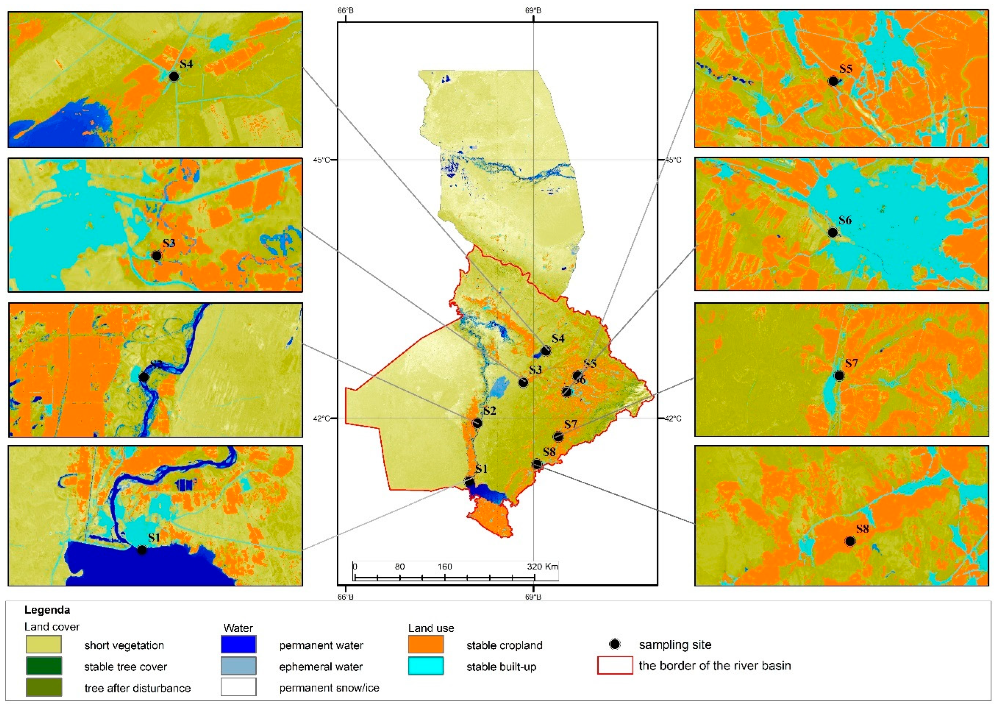
Disclaimer/Publisher’s Note: The statements, opinions and data contained in all publications are solely those of the individual author(s) and contributor(s) and not of MDPI and/or the editor(s). MDPI and/or the editor(s) disclaim responsibility for any injury to people or property resulting from any ideas, methods, instructions or products referred to in the content. |
© 2025 by the authors. Licensee MDPI, Basel, Switzerland. This article is an open access article distributed under the terms and conditions of the Creative Commons Attribution (CC BY) license (https://creativecommons.org/licenses/by/4.0/).