Abstract
In geosciences, soil–water interactions are defined by soil water potential, which provides a quantitative estimate of the soil water thermodynamic state. Due to the interactions between water and soil particles, soil water has different physical properties than free water; hence, analyzing soil water may require different methods and approaches. Typically, soil water potential is defined as the sum of three independent functions: gravitational, osmotic, and matric. However, there is a problem with this definition because the osmotic and matric potentials exhibit coupling effects. Moreover, due to its high values, the matric potential dominates the total potential, whereas the gravitational potential may appear negligible. However, gravity may lead to different flow mechanisms altering the soil’s mechanical behavior. As a result, it may not be valid to calculate the total water potential as the algebraic sum of the different potentials. There are also mathematical challenges in the common use of water potential; as soil saturation decreases, water potential can reach thousands of kPa, which requires mathematical balancing in the equations by multiplying it by a variable with a value near zero. However, multiples of numbers of different magnitudes are problematic from a mathematical perspective, especially when applied to numerical analysis. This paper discusses the strengths and limitations of the definitions and mathematical formulations of this variable.
1. Introduction
Soil water potential plays an essential role in defining soil–water interaction. In geosciences, the soil water potential value gives a quantitative estimate of the thermodynamic state of soil water, and it is a fundamental parameter in biology, chemistry, and physics.
Soil water potential controls various biological processes occurring through and across the soil–plant–atmosphere continuum [1,2,3,4,5]. There are a number of bio-physical processes that are influenced by soil water potential, including seed germination and plant growth. Gradients in soil water potential are the driving forces of water movement, affecting water infiltration, redistribution, evaporation and plants’ transpiration [6]. Monitoring soil water potential is useful for improving irrigation efficiency and designing water-saving irrigation systems [7,8].
In hydrology and hydrogeology, soil water potential is used to quantify water flow in unsaturated soils [9,10]. Water potential drives both convection (movement of the bulk solution including all phases) and diffusion (movement of water alone) [11,12]. In soil formation, groundwater flow affects dissolution and precipitation processes [13]. Water potential plays a significant role in soil mineralogy and sedimentology [14], which in turn affect structural geology [15].
Water potential plays an important role in a wide range of multiphase processes, including simultaneous movement of air and water, simultaneous transport of moisture and heat, water movement in shrinking and swelling soils, and solute transport in unsaturated soils [16].
In geological engineering, the soil water potential parameter can be used as a tool for identifying mechanical stress and volumetric changes in unsaturated soils. Based on the soil’s water potential, unsaturated soil’s constitutive laws are usually extrapolated from saturation conditions. Effective stress, defined in terms of water potential, is often assumed to determine mechanical behavior in unsaturated soils [17,18,19,20,21,22].
In other scientific disciplines, it has been shown [23,24] that the relationship between temperature and soil water potential can be used to described coupled water and heat transport. By using the water potential, it is possible to distinguish between two paths by which electrical currents flow in clayey soils: the liquid phase (free water) and the surfaces of electrocharged clay minerals absorbed in water [25].
This paper presents an overview of soil water potential, including definitions and applications in several geoscience disciplines. This paper discusses the strengths and limitations of the definitions and mathematical formulations of this variable. A number of the current concepts of matric suction, pore water pressure, and effective stress are not physically and mechanically precise enough for solving practical geotechnical and environmental engineering problems; a lack of clarity in concepts and an understanding of their limitations may lead to inadequate physical representations of soil–water interactions. Water potential is an energy potential variable, but it is also often used as a pressure variable; this causes difficulties in the mathematical formulation and theory.
2. Abnormal Behavior of Absorbed Soil Water
The soil water potential is a parameter that characterizes the potential (energy) of the water absorbed by the soil. In absorbed water, molecules of water are chemically bound to solid surfaces of soil particles. The absorbed water possesses different physical properties than free (bulk) water. Free water in an external environment (1 atm) is expected to freeze at 0 °C, have a density of 1 g/cm3, and follow the phase diagram. From the perspective of the phase diagram (Figure 1), when water’s pressure decreases, it transforms from a liquid to a vapor, and specifically, water cannot exist in tension at equilibrium.
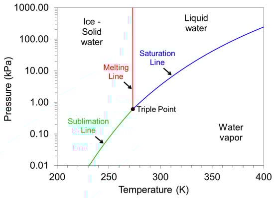
Figure 1.
Free water phase diagram.
The water absorbed by soil, however, does not follow any of the above rules. Interlayer water in clayey soils has several characteristics that are quite different from free water. In soil pores, water does not freeze at 0 °C; instead, its freezing point is depressed because of interactions between soil particles, solutes, and water [26]. Furthermore, water adsorbed on clay surfaces was determined to have a density greater than 1.4 g/cm3 in low-water content conditions (as shown in Figure 2) [27,28]. This high density is caused by an abnormally high adsorption potential occurring near soil particle surfaces or within clay’s interlayer spaces. In contrast, surface tension produces tensile pressure at the air–water interface, stretching the water molecules’ bonds, resulting in a slight decrease in the density (0.995 g/cm3) [29].

Figure 2.
Adsorbed water density curve of Na-montmorillonite, after [27].
Considering what has been described above, analyzing absorbed soil water may require different approaches and techniques than analyzing free water. The solid matrix is responsible for the different behavior of absorbed soil water; therefore, it is crucial to identify how water interacts with soils, particularly clay soils, which have a strong interaction with water because clay sheets have negatively charged surfaces that bond with water molecules. In terms of mineralogical and chemical structures, clay has two basic structural units: tetrahedral and octahedral. In the tetrahedral unit, four oxygen atoms are arranged in a tetrahedral shape around a silicon atom. In the octahedral unit, six hydroxyl ions (OH-) or oxygen are arranged in a hexagonal shape around an atom of aluminum, iron, or magnesium (Figure 3). Clay minerals (including kaolinite, illite, and montmorillonite) are composed of these basic clay structure units, and the negative charge layer arises from isomorphic substitutions of tetrahedral or octahedral metals [30,31]. A common clay mineral in expansive clay soils is montmorillonite, which attracts cations due to its negative charge, and due to the weak bond between individual montmorillonite units, water can penetrate between the sheets and cause separation and swelling [32]. Water is attracted to soil because of its soil water potential, which is characteristic of clay minerals. Often, water potential is referred to as soil pore water pressure, water tension, or soil suction.
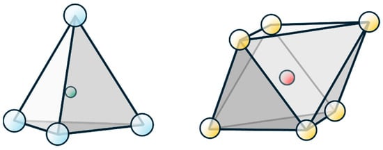
Figure 3.
Tetrahedral unit (four oxygen atoms around a silicon atom) and octahedral unit (six hydroxyl or oxygen around a metal atom).
3. Definition of Soil Water Potential
Using vertical soil columns, Briggs [33] tested the ability of soil to retain water based on the interaction between capillarity and gravitational forces. Early in the twentieth century, soil physics developed the study of soil suction. The energy concept was introduced to soil physics by Buckingham [11], who defined soil water potential as the amount of work needed to pull water away from soil. Buckingham identified soil’s ability to retain water as capillary potential, which represents the soil’s ability to attract water at a given point.
Due to the fact that soil water potential represents potential energy, it should be expressed in terms of energy per unit mass or volume of water. It is typically expressed in units of pressure, such as megapascals (MPa) or kilopascals (kPa).
In accordance with the Buckingham concept, the I.S.S.S. (the International Society of Soil Science) in 1963 defined the total water potential as the energy state of water in soil as follows [34]:
“The amount of work that must be done per unit quantity of pure water in order to transport reversibly and isothermally an infinitesimal quantity of water from a pool of pure water at a specified elevation at atmospheric pressure to the soil water (at the point under consideration)”.
Researchers (e.g., [35]) later concluded that this definition might have some deficiencies. A few years after Buckingham introduced the energy concept, by using thermodynamic functions, soil science researchers were able to better define soil water potential; thermodynamic functions can express water’s energy changes over a wide range of soil conditions. As a result, the I.S.S.S. updated its definition of total water potential from a thermodynamic perspective [36]:
“The total potential, , of the constituent water in soil at temperature , is the amount of useful work per unit mass of pure water, in J/kg, that must be done by means of externally applied forces to transfer reversibly and isothermally an infinitesimal amount of water from the state to the soil liquid phase at the point under consideration”.
The reference state represents water at the reference plane, unaffected by dissolved salts (zero osmotic pressure), free (unaffected by a solid phase), at temperature , and exposed to atmospheric pressure; i.e., while the test body of water is being transferred, the force fields acting on it determine the total potential. Generally, these forces are gravity, pressure gradient force, diffusion force, and electrical adsorption force. The potential is negative when the soil adsorbs water from the reference state. In any soil–water system in a state of rest, the total potential does not vary from point to point in the system [37].
4. Mathematical Formulation
A calculation of the soil water potential, can be made by adding up various components corresponding to different mechanisms (Equation (1)); i.e., the work done against these forces (e.g., [1,6,38,39]): (i) the gravitational potential caused by the gravitational field, (ii) the matric potential caused by solid-water interactions in the soil, and (iii) the osmotic potential caused by electrolytes and solutes dissolved in water. In some cases, the total potential expression may include additional terms.
Gravitational potential is determined by the soil water elevation relative to the chosen reference elevation. Matric potential is determined by capillary and adsorptive forces exerted on water by the soil matrix (soil particles). The osmotic potential is determined by the solutes dissolved in water, as polar water molecules are attracted to electrolyte cations and anions because of the hydration force.
Traditionally, soil water potential was decomposed into the three independent functions of gravitational potential, matric potential, and osmotic potential. However, the actual situation is more complex; matric and osmotic potentials are not independent but rather related to the soil–water interaction, creating a coupling between the two [39].
Matric potential refers to the change in the energy state of water in soil caused by physicochemical interactions between water molecules and soil particles. Matric potentials can range from zero to thousands of kPa, which makes it the primary factor in determining the total soil water potential. In particular, gravitational potential in soil systems is generally not significant, except when dealing with large-scale issues. For example, an elevation change of 1 m height leads to a gravitational potential of about 10 kPa, which is far less than the other components of soil water potential, and therefore is allegedly negligible [39]. As matric potential is probably the primary factor component of soil water potential, it is discussed in greater detail below.
5. Matric Potential—Capillarity and Adsorption
The matric potential refers to the soil matrix’s chemical potential in the three phases of soil–water–air interaction systems via capillarity (mechanical) and adsorption (physicochemical). In capillarity, a curved air–water interface (i.e., a meniscus) exists between the solid, water, and air phases; the water meniscus forms at the edges of the solid phase and shows a convex curvature towards the air phase. Water rises due to surface tension in the meniscus. Pore diameter and surface tension determine the height of this rise. When the pores are larger, capillary rise is minimal, whereas when pores are smaller, it is more pronounced. Therefore, the capillarity of the soil is determined by its texture. Because coarser soils have larger pores, capillary forces are weaker, while fine-textured soils have strong capillary forces. The capillarity is a mechanical mechanism in nature [40]. However, the mechanisms for adsorption, which include surface hydration, interlayer hydration, and multilayer adsorption, are all electromagnetic mechanisms in nature. Water molecules are attracted to the surfaces of soil particles, creating a thin film of water around the particles that is tightly held by electromagnetic forces. Water molecules are bound to soil particles at the molecular level (Figure 4). Adsorption occurs especially in soils with a high clay content, high specific surface area, and more charges. In contrast, sandy soils with a lower surface area and fewer charges have less adsorption. Mathematically, the matric potential is the superposition of capillarity potential and adsorption potential.

Figure 4.
Schematic of an unsaturated pore space showing the capillary and adsorbed water films.
Compacted clay is typically characterized by a double pore structure (Figure 5); macropores (large pores) are located between the pods, while micropores are located within the pods [41,42,43]. It has been discussed previously that water flows through macropores and micropores in different mechanisms (e.g., [44,45,46]). In comparison to macropores, micropores exhibit higher suction forces and lower hydraulic conductivity. In compacted soils, it has been found that the volume of the micropores is not altered by the compacting process; however, macropores are decreased in quantity and size due to compacting [47]. Reduced macropore counts disrupt preferential flow pathways, resulting in reduced permeability [48].
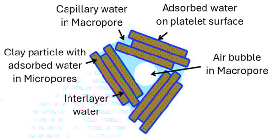
Figure 5.
Double pore structure, after [49].
Baker and Frydman [49,50] suggested that according to the double porosity model, in fine-grained soils, the adsorption potential is often the dominant component of the matric potential, whereas the capillary potential is only significant at low matric potentials down to the cavitation tension. There can be no smaller capillary potential than the cavitation potential; at lower potentials, macropore water drains into the pods, and the matric potential is solely determined by the adsorption potential. At moisture contents below optimum, macropores are essentially empty of water, and the matric potential is solely due to adsorption forces in micropores. In a study by Pedrotti and Tarantino [51], micropore distribution was found to be similar to pores in slurry samples, and macropore distribution was found to be similar to pores in samples prepared from dry powder. This has led to a view of compacted soil’s microstructure, in which macropores are just air-filled pores and micropores are just water-filled pores.
Based on the above, it appears that adsorption dominates soil–water interactions rather than capillary potential. Fine-grained soils, especially clays, generally have a large specific surface area, which favors water retention by adsorption. Additionally, clay minerals have negatively charged surfaces that attract positive cations to their surfaces and into interlayer spaces. Adsorption of water on soil particle surfaces is governed by five independent physicochemical mechanisms (all are electromagnetic in nature), including electrical field polarization, electrical double layers, van der Waals attraction, cation hydration, and hydrogen bonding. A detailed explanation for each individual component of the matric potential can be found in [39].
In many cases, researchers (e.g., [52,53,54,55]) have explained the matric potential by comparing pores in soil to capillary tubes with small radiuses. As a result of soil capillaries, absorbed soil water rises above the water table. Capillary water has a negative pressure when compared with air, which is generally atmospheric (as shown in Figure 6). Based on this logic, matric suction is commonly defined as the difference between the pore air and the pore water pressures, as shown in Equation (2) (e.g., [17,18,20,21]):
where and are the pore air and water pressures, respectively.
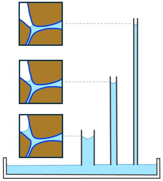
Figure 6.
Air–water interfaces in capillary tubes of various diameters and their equivalents in soils, after [52].
This identification of matric potentials as capillary potentials is incorrect, since it ignores all physicochemical mechanisms associated with water adsorption on soil surfaces and within the interlayer space. As a matter of fact, it is impossible to define the matric potential logically without considering the soil as soil rather than capillary tubes. Furthermore, the matric potential is by definition energy per unit volume, not pressure. The capillarity potential, which is a mechanical mechanism, can be expressed mathematically as pressure, but not the adsorption potential, which is an electromagnetic mechanism. However, despite these shortcomings, this idea is extremely popular and is the basis for measuring water potential using axis translation, as described next. Furthermore, it is possible that this popularity is a result of axis translation being the main experimental technique used to study unsaturated soil behavior in the previous decades [49]. Essentially, Equation (2) represents water potential as pressure and therefore retreats from Buckingham’s definition of water potential as energy.
6. Soil Water Potential Measurements
The soil water potential measurement has been discussed many times in the past (e.g., [7,38,56,57,58]). Three categories of techniques are commonly used in lab and in situ experiments based on the phase of the sensing material: solid-based (e.g., filter paper), liquid-based (e.g., tensiometer and axis translation), and vapor-based (e.g., hygrometer).
Filter paper: A porous medium, such as Whatman No. 42 filter paper, is brought to equilibrium with a soil sample either directly in contact (for matric potential) or in closed systems without contact (for total potential). Water potential is determined based on the moisture characteristic curve of the filter paper after the natural water content of the paper is measured using a drying oven [59]. In the middle range of water potentials, the filter paper method is relatively accurate; however, it is less accurate at the edges of water potentials (extremely dry or wet soils). The method requires isothermal conditions, which is not always easy to accomplish and may cause significant errors if small temperature variations occur. In general, filter paper methods are indirect, time-consuming, and difficult to automate, despite being simple and affordable.
Tensiometer: The basic elements of the tensiometer include a small water reservoir connected to a high air entry value porous stone on one side and a membrane instrumented with strain gauges on the other. Through the porous stone held directly in contact with the soil, water moves from the reservoir to the soil until it has equal energy on both sides. As a result, the membrane is tensed by a vacuum in the reservoir Tensiometer data is commonly interpreted by identifying the measured water tension with soil water tension. It should be noted, however, that at equilibrium, it is the water potential, not the water pressure, that is equal across the system. Hence, these instruments actually measure the potential energy of soil water rather than the mechanical stress. Water molecules and solute molecules pass through the porous stone, which isolates solids and air from the water reservoir; as a result, the tensiometer measures matric potential. Water inside the reservoir determines the range of the tensiometer by its capacity to resist a vacuum without cavitating. Cavitation occurs when the strong bonds of water are disrupted by surface discontinuities, such as edges or grit, which can provide nucleation points causing cavitation (which is discussed in more detail in the next chapter). Basic tensiometers cavitate at around −80 kPa. Novel tensiometers (e.g., [60,61,62]), however, have a much greater range thanks to precision engineering and meticulous construction. The devices, however, have difficulty maintaining long-term measurements due to their use of a balance in a metastable condition, as explained later.
Axis translation: In the axis translation technique, air pressure is applied to the soil to increase the pore water pressure and shift it to be positive, preventing cavitations in water drainage systems [63]. The soil water pressure is artificially increased, and the air water pressure difference is determined as the water potential. Generally, the total stress on the soil is increased simultaneously with air pressure to maintain a constant net stress (total stress minus air pressure). In unsaturated soil testing, axis translation has become the most popular method for measuring or controlling matric water potential [64]. This method provides reliable accuracy measures when calibrated properly. However, there is a fundamental limitation in the axis translation, which is that the soil’s behavior is changed by it. In contrast to field conditions, in which atmospheric pressure is usually present, applying external air pressure to unsaturated soil changes the state of the soil, thereby altering its mechanical behavior [49,50].
Hygrometer: Hygrometers measure vapor pressure, i.e., relative humidity (), which is a measure of water potential (Equation (3)). Relative humidity is measured in soil at thermal equilibrium, and converted to water potential. Water is evaluated in two equilibrium systems, the absorbed soil’s water and the air’s water (humidity). Humidity is the concentration of water vapor present in the air, whereas relative humidity is the ratio of how much water vapor is in the air to how much water vapor the air could potentially contain at a given temperature. Refining a reference state (e.g., without environmental factors), once the soil–water system is in equilibrium with water vapor in the environment, the thermodynamic relationship of the water potential can be written as follows (e.g., [55,65]):
where is the universal gas constant (8.31432 J/(mol K)), is the absolute temperature (K), is the molar volume of water (1.8 × 10⁻⁵ m3 mol−1 at a standard temperature and pressure), and is the relative humidity.
A graphical representation of Equation (3) for 30 °C can be found in Figure 7.

Figure 7.
Thermodynamic equilibrium between relative humidity and total suction at 30 °C.
The use of hygrometers for analyzing soil samples in powder form has been found to be a powerful tool, and vapor sorption analyzers are presently used to create moisture sorption isotherms and wetting–drying cycles (e.g., [66]). This method, however, is usually more suitable for distributed samples, as it cannot control confined stress or monitor soil density as moisture changes. The method is generally considered accurate, but when the relative humidity is high, it can be difficult to measure, resulting in inaccurate results for wet soils.
Another semi-empirical method for measuring water potential is by using heat dissipation sensors and dielectric sensors. A heat dissipation sensor consists of a porous ceramic cup with an embedded heating element and a temperature sensor. Once the ceramic cup has been placed in the soil, the pores in the ceramic cup will eventually reach equilibrium with those in the soil around it. A heating element is heated for a specified time interval, with the temperature sensor monitoring the change in temperature. Temperature changes in ceramic cups are time-dependent due to their thermal conductivity, which is dependent on their water content. By comparing the water content with the ceramic’s water retention curve, it is possible to determine the water potential of the cup, which is in equilibrium with the soil around it. In dielectric sensors, porous ceramic cups are placed in the soil and reach equilibrium with the soil in the same way as heat dissipation sensors. Instead of measuring thermal properties, these sensors measure the dielectric properties of the ceramic cup (dielectric permittivity). Measurements of dielectric properties can either be done in the time or frequency domain or by measuring the dielectric properties of the cup. Dielectric properties are determined by the water content, which is related to water potential through the retention curve. These methods are generally considered to be less accurate due to their semi-empirical nature.
For nearly all practice problems, water potential is determined using the above techniques. In flow equations, for example, the water potential is used to calculate the gradient. While this approach is sufficient to describe water movement in macropores (where capillarity is dominant), it will produce considerable errors in fine-grained soils characterized by micropores, since the local intermolecular water pressure cannot be directly measured due to current technological limitations. It is a matter of scale, since these devices measure bulk water pressure averaged over pores with sizes ranging from microns to millimeters at least.
7. Cavitation
The cavitation phenomenon is fundamental to the understanding of soil water potential. Generic tensiometer limitations are caused by the cavitation phenomenon. Additionally, the cavitation phenomenon led to the development of the axis translation method, in which high air pressures are applied to prevent water pressure from reaching a negative level, resulting in cavitation. The purpose of this chapter is to explain the cavitation phenomenon in more detail. Cavitation occurs when water reaches negative pressure, resulting in small bubbles that collapse easily. Therefore, cavitation can cause problematic wear and tear on propellers and pumps when repeated cavitation events are created near metal surfaces. According to this theory, water exhibits low tensile strength, causing it to cavitate and tear at low pressures.
Understanding the cavitation and boiling processes of water requires an understanding of bubble formation. Bubbles develop as part of the nucleation process. In physics, nucleation is the beginning of a phase transition or phase separation. Nucleation sites are the points at which phase transitions begin [67]. Differentiation between heterogeneous nucleation and homogeneous nucleation can be seen; heterogeneous nucleation occurs at discontinuities in the matrix on a preferred surface, while homogeneous nucleation occurs uniformly in the matrix. For example, in the nucleation of ice from supercooled water droplets, purifying the water to remove all impurities results in water droplets that freeze around −35 to −40 °C. However, when the water contains impurities, it may freeze at a much higher temperature because the impurities reduce the height of the energy barrier to nucleation [68]. Water impurities can be dust grains or simply surface contact, which makes heterogeneous nucleation much more common than homogeneous nucleation. Cavitation and boiling are two types of nucleation. Cavitation occurs when the pressure falls below a critical level, and boiling occurs when the temperature rises above a critical level.
Berthelot studied the tensile strength of water in 1850; Figure 8 illustrates his experiment [69]. Berthelot filled a cylindrical glass tube with water at room temperature, leaving a small volume of air at the end of the tube (stage 1 in Figure 8). Because water vapor in the air is in equilibrium with liquid water, it lies on the equilibrium line (coexistence line). In thermodynamics, equilibrium lines are the boundaries between phases along which two phases can exist simultaneously in equilibrium, such as water and water vapor. When the cylindrical glass tube was heated, it expanded more than the glass tube, since water’s thermal expansion coefficient was higher than the glass’s thermal expansion coefficient (stage 2). Eventually, the heating forced the all the air to dissolve in the water (stage 3). As the tube cooled, it tended to contract and the water “stuck” to its walls and tensed (stage 4). Suddenly, the tube’s volume increased with a “click” sound, revealing gas in the tube (stage 5). Essentially, this click was caused by cavitation. Since the water and the glass had different thermal expansion coefficients, the water reduced its volume more than the tube due to cooling. Yet, the water and the tube were forced to reduce their volumes identically as a result of their adhesion. Consequently, water stretched until it “broke” and cavitated. It is possible to determine the tension force prior to cavitation by measuring the tube volume change before and after the click. In fact, this tension force is water’s tensile strength. Berthelot’s experiment was the inspiration for the tensiometer device [70].
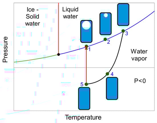
Figure 8.
Berthelot tube, after [69].
Based on Berthelot’s results, water can exist at low pressures and even under tension in a state of equilibrium beyond the standard phase diagram. Usually, when the equilibrium line between phases in the phase diagram is crossed, the material will change its phase. When the pressure on liquid water is reduced, the liquid–vapor equilibrium line is crossed, and the most stable phase of the water will be vapor. There is, however, an energetic barrier in the transition of liquid to vapor, which allows for a “metastable liquid” [71,72]. In order for the phase transition to occur, the vapor bubbles must nucleate, which requires additional energy. An energy profile is shown in Figure 9 for stable, unstable, and metastable states. The metastable state is separated by a small energy barrier. Metastable states rarely occur because random fluctuations are large enough to overcome energetic barriers. However, at the nanometer level, the barriers are large relative to the system size, so metastable states may last for a long time. This is known as the “scale effect”. The Berthelot tube shows that phase changes can be postponed even at the macro level if nucleation is prevented by special measures.

Figure 9.
Schematic of an energy profile of a system showing stable, unstable, and metastable equilibriums (separated by a very small energy barrier), after [71].
Based on hydrogen bonds in water, it can be estimated that the tensile strength of pure water can reach up to 160 MPa or more [73,74]. In order to describe these tensile forces, physicists proposed the updated phase diagram (Figure 10), where the critical spinodal pressure corresponds to the tensile strength of liquid water at a given temperature. This phase diagram revision is not as unusual as it may seem; water absorbed in soil has a different nature from free water and does not follow free water’s rules, so it makes sense that their phase diagrams would differ. Furthermore, the common phase diagram (Figure 1) is only a private case when the volume is constant. An accurate description of the phase diagram requires a three-dimensional (3D) graph of three thermodynamic quantities. Three-dimensional graphs of this type are called p-v-T diagrams since they include temperatures (T), pressures (p), and volumes (v). Equilibrium lines become curved surfaces when transformed into 3D. Orthographic projection of the 3D p-v-T graph can be used to convert the 3D plot into the standard 2D pressure–temperature diagram [75,76]. Soil-absorbed water has a much higher density than free water, so it is unlikely that it will fit the classic phase diagram.
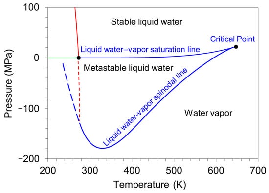
Figure 10.
Water stability diagram with localization of the metastability zone associated with tensile stabilized water, after [72].
Following the definition of water potential in soil, this paper discusses two disciplines in the geosciences field where water potential plays an important role: flow equations and geotechnics. In light of the above definitions, this paper examines how these two disciplines use water potential and discusses the problems associated with their common application.
8. Flow in Unsaturated Soil
In unsaturated non-swelling soil, the basic flow equation provides the volumetric water content, (defined as the ratio of the water volume to the total soil volume), as a function of the flux, , which enters and exits a control volume [77]. Assuming that the density of water is constant in time and space, the equation obtained is:
Equation (4) contains two variables, and ( has three components in three orthogonal directions), and therefore it cannot be solved alone. This requires an additional relationship between these variables, and a methodology based on Darcy’s law [78] is commonly used to describe the water flow.
Equation (5) shows the original form of Darcy’s law:
where is the permeability, and is the hydraulic head.
Darcy’s law was developed based on empirical evidence for saturated flows through sand; for clayey soils, and especially for unsaturated flows, this law may not be valid. However, the law has been applied to unsaturated flows (e.g., [79]) and even to non-rigid soils when solids move with liquids (e.g., [80]). To implement the law in these cases, the hydraulic head is replaced by the soil’s water potential (Equation (6)) [81,82].
In saturated flow, is constant over a wide range of hydraulic heads. In fact, Darcy was the first to discover that is constant, and that is what forms the basis of his law. However, this is not true in unsaturated flow; in unsaturated flow, varies with water content. It is generally assumed (e.g., [43,83,84]) that is equal to the saturated permeability multiplied by a function of the water potential or the volumetric water content. In the case where the volumetric water content function is selected, another equation connecting the water content to the water potential is required; this equation is the water retention curve (Figure 11).
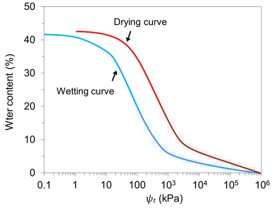
Figure 11.
Schematic water retention curve., after [55].
The water retention curve is the relationship between volumetric water content and soil water potential. Due to clay soil’s large surface area and small pores, it retains water even at high (negative) matric potentials. As a result, the curve declines relatively gradually, where a relatively small change in water content results in a relatively small change in water potential. In contrast, sand, which has larger pores, has a steeper water retention curve. Sand retains water in a relatively narrow range of low matric potentials; sand drains rapidly under gravity and cannot hold as much water at high matric potentials—where the retention curve becomes flat. Hysteresis occurs in the water retention curve when water fills and drains the pores, resulting in different wetting and drying curves.
A number of limitations are associated with the above method:
- Retention curves are based on equilibrium states rather than flow states and therefore must be altered to match non-equilibrium conditions (e.g., [85]). In addition, the retention curve is affected by the soil properties (density and void ratio) [86] and confined stress history [55,87,88], parameters that are not taken into account in the majority of cases. Moreover, in some cases, the hysteresis between wetting and drying cycles is not taken into account. Pitfalls in the interpretation of the gravimetric water content-based soil water characteristic curve for deformable porous media were reviewed by [89].
- There are some limitations to Darcy’s law, primarily for macroscopic and multi-phase fluid flow [90]. In particular, experiments [91,92,93] indicated that Darcy’s law is not valid for describing water flow in clayey soils due to highly non-linear relationships between water flux and the hydraulic gradient. Moreover, assumptions built into the law [90] need to be considered. These limitations are not taken into account in many cases.
- As soil saturation decreases, water potential can reach thousands of kPa (especially in clayey soils). A water potential with an extremely high value is accompanied by a high value derivative ( in Equation (6)); therefore, in order to obtain a reasonable water flux, it is necessary to multiply the enormous water potential by a nearly zero permeability (e.g., [43,94,95]). For example, Figure 12 shows the relative water permeability, which is the permeability in unsaturated conditions relative to saturated conditions for Boom clay (after [43]). However, multiple different magnitudes are problematic from a mathematical perspective, especially when applied to numerical analysis [96,97].
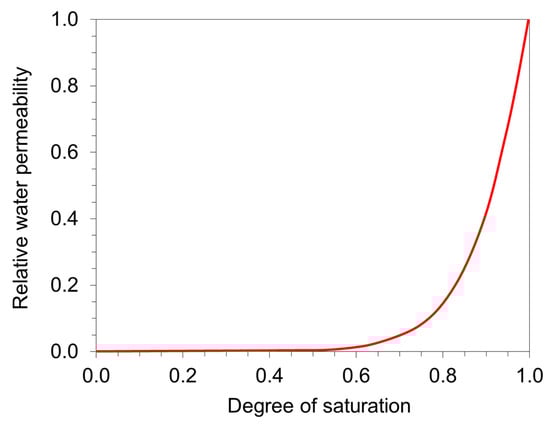 Figure 12. Relative water permeability–degree of saturation relationship for different packings at constant porosity for Boom clay at dry unit weight of 16.7 kN/m3, after [43].
There are several equations in the literature that describe retention curves, which are all based on empirical parameters that need to be calibrated for the specific soil. An equation commonly used is the Van Genuchten equation [98] because it can be adapted to a variety of soil types and retention curves. However, this equation is so flexible that it can be used with any set of measurements, even if they are not reliable measurements. Therefore, fitting between measurements and the equation does not prove the accuracy or validity of the measurements or the method. Brooks and Corey’s model [79] is another common empirical model used to describe the relationship between soil water content and matric potential. The model is simpler than the Van Genuchten model and is particularly useful for predicting soil water retention in coarse-textured soils. Assouline and Or [99] provided a review of the primary models and highlighted their physical basis, assumptions, advantages, and limitations. Updated models can be found in the literature, and some are based on hundreds of soil surveys and on advanced machine learning methods (e.g., [100,101,102]).
Returning to the flow equation, the equations and mathematical relationships between these different parameters are semi-empirical, nonlinear, and vary from soil to soil. A numerical solution to a nonlinear problem must be updated throughout the solution as the water content changes. Numerical techniques are applied in increments of space and time (e.g., [103]). Numerical solutions require soil parameters as inputs, so they must be calibrated based on soil type, boundary conditions, and initial soil conditions. Thus, solving flow problems under unsaturated conditions is a complex task.
Recent studies on unsaturated soil flow have combined an experimental framework with analytical analysis, focusing on small-scale problems and unique laboratory conditions (e.g., [104,105]). However, it is unclear how this state applies to real soil scales in situ considering that the adsorptive water flow in small pores is very different from the capillary water flow in large pores.
9. Flow in Swelling Soil
In non-rigid soil, solids are moved along with liquids. When the soil volume changes, it affects the flow equation, resulting in coupled problems. When adapting Richard’s theory to non-rigid soils, the solid phase is used to reference the water flux. Eulerian or Lagrangian frameworks can be used to describe fluid flow in a non-rigid porous medium, with the former using a fixed coordinate system (e.g., [81]) and the latter using a material-related coordinate system (e.g., [80]).
A Eulerian approach refers to the motions of water and solids in reference to the fixed coordinate system (e.g., [106,107]). According to this approach, two water fluxes are defined: an absolute water flux based on the fixed coordinate system and a water flux that flows through soil pores; for the latter, Darcy’s law is assumed to be valid.
In the Lagrangian approach based on material coordinates, water flow is defined in relation to the soil’s solids (e.g., [80,108]), and Darcy’s law is considered valid to describe water flow. However, there is still a need to describe the movement of the solids themselves.
As demonstrated by Philip [106], even though these two approaches produce different equations, they are, in fact, physically identical. Regardless of the method used for solving water flow equations, it is necessary to define how solids move as water advances.
When soil is saturated, solids’ motion can be correlated with the change in volumetric water content (e.g., [106]), resulting in a relationship between water and solid movement. Unlike saturated soil, unsaturated soil contains air within voids, so solid movement is determined by changes in the void ratio rather than the volumetric water content (e.g., [108]). Consequently, there is no one-to-one correspondence between the movement of water and solids. As a result, solids’ movement in saturated flows (two-phase), and even more so in unsaturated flows (three-phase), is complex to analyze.
When describing water movement, Keissar [109] proposed that the flux of solid particles relative to the fixed coordinate system can be negligible. Thus, water distribution in swelling soil caused by infiltration flows is similar to that in stable soils; the main difference is the rate of flow rather than its characteristics. Other approaches (e.g., [110]) suggest that swelling soils have a different water distribution than stable soils.
According to Yong [111], expansive soils that swell during infiltration have lower infiltration rates than rigid soils. In the case of expansive soil that is confined, the rate is even lower. In fully confining conditions, where volume changes are not allowed, the flow rate is the smallest (Figure 13). Therefore, in solving flow equations, confining stresses must be considered. Furthermore, unsaturated clay’s permeability was found to be stress-dependent [112], i.e., the parameters of the soil itself are stress-dependent. Water flow is affected by changes in the volume and stresses of the soil, while the volume and stresses of the soil are affected by water flow, resulting in coupled problems. Geomechanics and multiphase flow in porous media are fundamental problems in geotechnical engineering. The mathematical formulation of this problem is used in surface displacement, hydraulic fracturing, borehole collapse, etc. Typically, soil behavior can be described mathematically as a constitutive law that includes strain and stress tensors as well as soil parameters and water content. Due to the fact that water in soil is neither constant in time nor uniform in space, it is necessary to have a tool to track its state in order to formulate the constitutive law; flow equations are generally used for this purpose. As soil volume changes, the flow equation is affected, which results in coupled problems. Recent advances in computer and numerical capabilities have enabled the development of numerical methods for solving coupled geomechanics and multiphase flows (e.g., [113,114]). Surprisingly or not, Darcy’s law remains an integral part of these models (e.g., [115]).
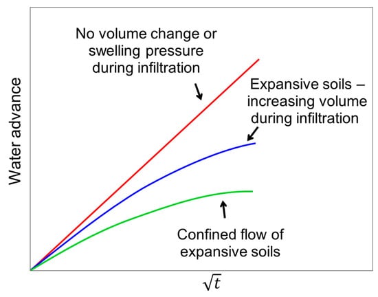
Figure 13.
Rate of wetting front advance showing the influence of volume change and confinement, after [111].
10. Soil Water Potential in the Geomechanics Field
Significant volume changes in clay soils in response to wetting and drying is a well-known phenomenon. These soils shrink and crack as they dry and swell as they wet. Volume changes in clay soil due to wetting or drying are a major source of damage to buildings, infrastructures, and roads in many parts of the world, and can be severe and costly [116,117].
Unsaturated soils have attracted increasing interest since the 1950s. Generally, it is accepted that the soil water potential influences the mechanical behavior of unsaturated soils (e.g., [17,18,19,20,21,22,118]).
The total water potential is assumed to be the algebraic sum of the matric, osmotic, and gravitational potentials. As a result of its high values, the matric potential dominates the total potential, and therefore, in many cases, only the matric potential is considered. Bishop [118] proposed the earliest and most well-known single-valued effective stress relationship. This equation (Equation (7)) is commonly referred to as Bishop’s effective stress equation for unsaturated soils.
where is the effective stress (the stress controls the strain or strength behaviour of soil), is the total stress, and is a soil parameter related to degree of saturation and ranging from 0 to 1 (e.g., Figure 14). When soil saturation decreases in clayey soils, water potentials can reach thousands of kPa (e.g., Figure 11), while Bishop’s parameter may drop to almost zero (e.g., Figure 14). There are, however, mathematical problems with multiple parameters of different magnitudes [96,97].
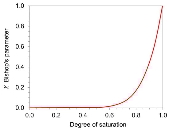
Figure 14.
Variation of Bishop’s coefficient with degree of saturation for highly active clay (Febex clay), after [119].
In Bishop’s equation, the water potential is represented as , where and are the pore air and water pressures, respectively; this representation is based on the logic shown in Equation (8).
The Bishop equation is an old model; however, is still discussed in the literature in updated studies (e.g., [119,120,121,122,123]). Likewise, advanced constitutive models define water potential similarly and determine effective stress from multiple parameters with different magnitudes. In most constitutive models, the water potential of unsaturated soils is expressed as air pressure minus water pressure (). Generally, this formulation is problematic (as detailed above), and specifically the identification of potential (energy per unit volume) with pressure (force per unit area) is problematic since these quantities possess different physical characteristics despite their similar dimensions [49].
Defining water potential as assumes that the water potential is equal to the matric potential capillary component, neglecting adsorption contribution, resulting in an unrealistic pore model [49]. It is likely that this definition was influenced by the laboratory axis translation technique; however, it is incorrect under typical field conditions, where air pressure is normally atmospheric, and cavitation prevents soil water from developing high tension. Axis translation changes the soil behavior by preventing cavitation, therefore making laboratory results from these tests less relevant to real-world conditions. There are many situations relevant to geotechnical engineering in which capillary potential seems to contribute only a small part to water potential, with water adsorption being the major contributor. The double porosity model and cavitation under tension should be taken into account when interpreting unsaturated soil behavior.
11. Numerical Methods of Unsaturated Soil Problems
The recent advancements in numerical methods for unsaturated soil mechanics have aimed at improving the accuracy, efficiency, and applicability of models used to simulate water flow (e.g., [124]), soil deformation (e.g., [125]), and other physical processes in unsaturated soils. These developments are critical for a range of geotechnical engineering applications, including soil stability analysis [125], groundwater modeling [126], irrigation management [127], and contaminant transport [128]. In agriculture, for example, new developments in numerical models have improved the simulation of evapotranspiration and root water uptake under varying environmental conditions. These models now use better representations of water stress, root distribution, and soil heterogeneity. The use of numerical methods has led to more accurate irrigation management recommendations through software, such as Hydrus-1D (4.16.0110) [129].
While traditional unsaturated soil models often separated hydraulic and mechanical processes, advances in Finite Element methods allow for the coupling of soil stress and water potential with mechanical deformation. This approach considers the effect of pore water pressure on soil deformation and vice versa, enabling more accurate predictions of unsaturated soil behavior under various loading conditions. These models have been used to simulate soil–structure interaction in unsaturated soils, particularly in the context of geotechnical slope stability [130], foundation settlement [125], and soil consolidation under drying and wetting conditions [131]. Constitutive models describe the relationship between soil stress, strain, and suction. Recent work has improved these models by incorporating nonlinearities [132] and hysteresis effects due to the different paths of soil response during wetting and drying cycles [133,134].
While the numerical methods for unsaturated soil mechanics have advanced significantly in recent years, each method has its own set of limitations and shortcomings. Understanding these limitations is crucial for selecting the right approach for specific applications and ensuring that models are used wisely. Coupling hydraulic and mechanical behaviors increases the complexity of the models. Solving coupled equations typically requires significant computational resources and longer computation times, especially for large-scale simulations. Advanced constitutive models, especially those that incorporate hysteresis or plasticity, are highly nonlinear. This nonlinearity can complicate both the solution process and the calibration of the model, requiring extensive experimental data to derive accurate material parameters. Due to these difficulties, the models often simplify complex soil processes and assume idealized boundary conditions. This can limit the models’ applicability in more complex real-world scenarios. Additionally, nonlinearity can lead to convergence issues during numerical solution. Accurate model predictions often depend on reliable experimental data for soil parameters, such as soil water characteristic curves, which may not be readily available or difficult to measure. Even with well-calibrated models, the inherent variability of soil properties (e.g., pore size distribution, degree of saturation) introduces uncertainty in the predictions, which can affect the models’ reliability. These models require detailed soil parameterization, such as root depth, soil texture, and soil water retention characteristics, which are not always available or easily measurable in the field.
The Discrete Element Method (DEM) in soil behavior modeling (e.g., [135,136,137]) is well-suited for small-scale or laboratory-scale problems, but scaling the method to model large volumes of soil or whole fields can be computationally impossible. The need to simulate each individual particle’s behavior in large-scale models requires a massive amount of computational power. DEM models typically idealize the behavior of granular materials as rigid particles or simplified contact models. This simplification may miss important aspects of soil–water interactions, such as the effect of surface tension in capillary action. These models may struggle to accurately simulate large-scale heterogeneous systems.
Machine learning in soil behavior modeling (e.g., [138,139]) has become a growing trend in predicting and simulating soil behavior, including soil–water interactions. Data-driven soil models, such as neural networks, are being employed to predict soil water characteristics (like water retention or hydraulic conductivity) based on large datasets of soil properties. These data-driven approaches can enhance the efficiency of soil modeling. However, while machine learning and Artificial Intelligence models can make predictions based on data, they often lack physical insight into governing processes (e.g., capillary pressure–saturation relationships, soil deformation), making them less interpretable compared to traditional physics-based models.
In all the methods reviewed, water potential remains one of the most fundamental variables in the analysis of unsaturated soils.
12. The Effect of Gravity Potential
The total water potential is assumed to be the algebraic sum of gravitational, osmotic, and matric potentials. As a result of its high values, the matric potential dominates the total potential, and from a mathematical perspective, the gravitational potential may seem negligible in comparison to the matric potential. There is, however, no question that gravitational potential plays an important role in the flow mechanism. In fact, even models derived from Darcy’s law can simulate the gravitational potential’s importance. The water in the soil progresses through a wetting front that separates soil at initial moisture from soil at saturation. The wetting front represents areas where soil moisture changes incrementally, and their thicknesses vary with the flow of water. At the saturated edge, the matric potential is zero, and the gravitational potential is responsible for driving fluid flow.
The influence of the gravity potential on the water flow can be demonstrated using the tests described in [140,141]. Nachum et al. [140,141] examined the effect of gravity potential on wetting in montmorillonite clay specimens. An experiment with different gravity potentials was conducted with specimens measuring 63 mm in diameter and 21 mm in height with a dry unit weight of 14 kN/m3 under a vertical confining pressure of 30 kPa. Water was supplied to the specimen from a water reservoir seated on a digital weight balance, and the reservoir weight was recorded with time, indicating the rate of inflow of water to the specimen. A set of tests was conducted using different gravity potentials by creating a difference between the water level in the reservoir and the bottom of the soil specimen. The following discussion focuses on two conditions: (i) a gravity potential of 0 mm, in which the reservoir water level is the same as the specimen’s bottom (this condition is characterized by matric forces promoting water flow in the soil, while gravity forces oppose it), and (ii) a gravity potential of 60 mm, in which the gravity potential contributes positively to the water’s advance.
A WP4C device (METER Group, Inc., Pullman, WA, USA), based on Hygrometer principles, was used to determine water potential under these initial conditions; the water potential was approximately 3000 kPa, equivalent to 300 m of water height. In relation to 300 m, a level difference of 60 mm equals 0.02%.
Figure 15 shows the intake rate versus water intake, where the symbol h represents the gravity head. With an increase in gravity potential, the rate of flow into and through the specimen increases. For example, with a gravity head of 60 mm, 3 g of water flows at 0.1 g/min, while at a zero gravity head, it flows at 0.05 g/min, i.e., 50% less.
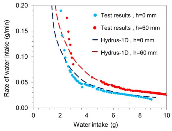
Figure 15.
Effect of gravity potential on rate of water intake, test results after [141].
A model based on Darcy’s law was examined using the Hydrus-1D software [129]. It is important to note that the numerical analyses performed using Hydrus-1D solved the flow problem for stable soils without considering volume changes. A number of empirical parameters must be defined as input parameters in the software. In this case, the parameters were adjusted based on the test results and the characteristics of montmorillonite clay. As illustrated in Figure 15, the software application can detect gravity potential effects in the experiment by utilizing flow models based on Darcy’s law. The fluid flow is continuous, and there is a correlation between different areas of the wetting front. The gravitational potential is the driving force at the saturated edge of the wetting front, and this edge affects the entire flow. Therefore, it seems that flow models based on Darcy’s law in unsaturated clays may work, even though the law is not valid for these conditions [91,92,93]. This does not prove that it is efficient or smart, but it at least works in many cases.
The gravity head differences affect not only the flow rate but also its nature. When water infiltrates under the gravity head, both macropores and micropores are filled with water, whereas infiltration under the zero-gravity head is only caused by capillary action in the macropores and subsequent adsorption in the micropores. Swelling is caused by adsorption into the micropores. Therefore, with an increasing externally applied hydraulic head, the vertical swell per unit quantity of water entering the specimen decreases. A positive external gravity head requires more water to produce a similar swell as adsorptive alone. Consequently, for a given quantity of water intake, a gravity potential of 0 mm will result in a larger swell. For example, for the tests described above in Figure 15, for 3 g of water intake, a gravity head of 60 mm would cause the soil to swell by 1.86%, while a gravity head of zero would cause the soil to swell by 2.13%. This has been described in more detail in [140,141]. However, when considering the cumulative swell magnitude, and not for a given quantity of water intake, a positive external gravity head will result in a larger amount of water being absorbed by the soil, hence resulting in a larger swell magnitude [140,141].
In geomechanics applications, since a minor change in gravity potential is expected to have a negligible effect on total water potential, its ability to affect the swelling magnitude in the constitutive models is limited. For example, Buzzi [142] proposed an equation for estimating volumetric strain using the soil initial water potential, confining stress, and initial void ratio. As a result, the elevation difference cannot impact the equation results, since it is negligible in the soil water potential. Although, the author [141,142,143,144] had found that minor changes in gravity potential may affect the soil swelling, both in its development and final magnitude. Nachum [145] conducted swell tests on montmorillonite clay under two wetting conditions, one where the specimen was inundated, and a combination of matric and gravity potentials assisted in the infiltration of water into the soil, and the other where water was brought into contact with the bottom of the soil sample, and water was absorbed in the soil due to matric forces only. The results indicated that different wetting conditions may lead to different swell magnitudes, where inundation conditions may cause greater swelling than adsorption. It was found that (i) as the initial void ratio decreases and (ii) as the initial degree of saturation increases, the difference between the swell caused by inundation and adsorption is greater. This phenomenon was explained by the unique mono-modal micropore size distribution expected under soil conditions with a low void ratio and a high degree of saturation [42]. Considering that micropores have a low hydraulic conductivity, the movement of water tends to be zero. Adsorption reduces the amount of water absorbed by the soil, which results in a lower volumetric strain. In contrast, when inundation occurs, water is applied to all the sample boundaries and may be absorbed into the soil without being dependent on matric forces. It is important to note that the increase in water intake, swelling, and swell magnitude was not limited to inundation but also correct when comparing cases when the soil was wetted from the bottom and the gravity potential was elevated by raising the level of the reservoir that supplied the soil with water, as shown and discussed in Figure 15 [140,141,143]. Wetting with a gravitational head of 60 mm had a very significant effect on the water intake and swell of soil with an initial head equivalent to about 300 m. How is this possible if water intake is due only to total potential?
The gravity head, which is commonly assumed to be negligible compared to the matric suction, becomes significant. In fact, inundation and adsorption have different water flow mechanisms. In porous media, different flow mechanisms have an enormous influence on the flow, for example, on the transport of contaminants by microorganisms in soils [144] and the multiphase flow in the oil industry [146]. Similarly, it is reasonable to conclude that different flow mechanisms may theoretically create different swell mechanisms. These results illustrate that the gravitational potential is not negligible. Therefore, calculating the total water potential as the algebraic sum of the different potentials cannot be valid.
A number of engineering guides restrict swelling potential to a certain value based on inundation tests (e.g., [32,147]). However, wetting conditions could have a significant impact on estimating the extent of damage to roads, structures, and infrastructure. Using the conventional design method, which involves inundation tests, may be economically inefficient. It may also damage roads due to different movements, such as when one section is flooded and the other section is only wet by suction. To provide a realistic estimate of swell, testing conditions should be equivalent with those expected in the field [145].
13. Summary and Conclusions
This paper presents an overview of soil–water interaction in geosciences from the perspective of the soil water potential parameter. The soil water potential gives a quantitative estimate of the thermodynamic state of soil water, and it is a fundamental parameter in biology, chemistry, and physics. It is possible to identify some weaknesses and fallacies in common perceptions of soil water potential, especially matric potential, and this paper aims to clarify incorrect perceptions. This work can be summarized as follows:
- Interactions between water and soil particles differentiate the physical properties of soil water from that of free water; water in soil pores does not freeze at 0 °C and can reach significantly higher density values than 1 g/cm3. Therefore, analyzing absorbed soil water may require different approaches and techniques than analyzing free water based on how the water interacts with soils.
- Soil water potential is typically defined as the sum of three independent potential functions: gravitational, osmotic, and matric, where three independent state variables are assumed to create the three independent potentials. This definition is questionable because osmotic and matric potentials exhibit substantial coupling effects. Furthermore, from a mathematical perspective, the matric potential dominates the total potential because of its high values, and the gravitational potential may appear to be negligible. Gravitational potential may, however, lead to different flow mechanisms that may alter the soil’s mechanical behavior. Therefore, calculating the total water potential as the algebraic sum of the different potentials may be not valid.
- By definition, soil water potential is an energy variable rather than a mechanical stress. It may not be an error to sum the matric potential with the gravity potential if the potential is a stress variable; however, since it is not a stress variable, it might be an error.
- In clayey soils, water potential can reach thousands of kPa as saturation decreases. When these conditions are considered in the flow equations, the potential of the water is multiplied by a permeability that is almost zero. Additionally, in constitutive laws in geomechanics, the water potential is multiplied by a coefficient with an almost zero value, such as Bishop’s parameter. However, multiple different magnitudes may be problematic from a mathematical perspective, especially when applied to numerical analysis.
- It is often suggested that the matric potential be defined analogously to the capillary potential (i.e., the difference between air pressure and water pressure) by comparing pores in soil to capillary tubes with small radiuses. In this definition, all the physicochemical mechanisms associated with water adsorption are ignored, i.e., the energy contribution from adsorption is not considered.
Funding
This research received no external funding.
Data Availability Statement
The original contributions presented in this study are included in the article. Further inquiries can be directed to the corresponding author.
Acknowledgments
I would like to thank and express my gratitude to Sam Frydman, who gave me the knowledge and insights on the topic of unsaturated soils. In addition, I would like to thank him for his insights and discussions in the preparation of this paper.
Conflicts of Interest
The author declares no conflicts of interest.
References
- Bhattacharya, A. Soil Water Deficit and Physiological Issues in Plants; Springer: Singapore, 2021; pp. 393–488. [Google Scholar]
- Boyer, J.S. Relationship of water potential to growth of leaves. Plant Physiol. 1968, 43, 1056–1062. [Google Scholar] [PubMed]
- Jordan, W.R.; Ritchie, J.T. Influence of soil water stress on evaporation, root absorption, and internal water status of cotton. Plant Physiol. 1971, 48, 783–788. [Google Scholar]
- Lafolie, F.; Bruckler, L.; Tardieu, F. Modeling root water potential and soil-root water transport: I. Model presentation. Soil Sci. Soc. Am. J. 1991, 55, 1203–1212. [Google Scholar]
- Ma, Y.; Liu, H.; Yu, Y.; Guo, L.; Zhao, W.; Yetemen, O. Revisiting Soil Water Potential: Towards a Better Understanding of Soil and Plant Interactions. Water 2022, 14, 3721. [Google Scholar] [CrossRef]
- Bittelli, M. Measuring soil water potential for water management in agriculture: A review. Sustainability 2010, 2, 1226–1251. [Google Scholar] [CrossRef]
- Bianchi, A.; Masseroni, D.; Thalheimer, M.; Medici, L.D.; Facchi, A. Field irrigation management through soil water potential measurements: A review. Ital. J. Agrometeorol. 2017, 22, 25–38. [Google Scholar]
- Yang, J.; Liu, K.; Wang, Z.; Du, Y.; Zhang, J. Water-saving and high-yielding irrigation for lowland rice by controlling limiting values of soil water potential. J. Integr. Plant Biol. 2007, 49, 1445–1454. [Google Scholar]
- Thamir, F.; McBride, C.M. Measurements of Matric and Water Potentials in Unsaturated Tuff at Yucca Mountain, Nevada (No. CONF-8511172-7); Goodson and Associates, Inc.: Denver, CO, USA; Western State Coll. of Colorado: Gunnison, CO, USA, 1985. [Google Scholar]
- Ringler, J.W. Monitoring the Hydrology of Soils for On-Site Wastewater Treatment Systems Using Matric Potential Sensors. Master’s Thesis, The Ohio State University, Columbus, OH, USA, 2009. [Google Scholar]
- Buckingham, E. Studies on the Movement of Soil Moisture (Bull. 38); USDA Bureau of Soils: Washington, DC, USA, 1907.
- Corey, A.T.; Kemper, W.D. Concept of total potential in water and its limitations. Soil Sci. 1961, 91, 299–302. [Google Scholar]
- Richardson, J.L.; Wilding, L.P.; Daniels, R.B. Recharge and discharge of groundwater in aquic conditions illustrated with flow net analysis. Geoderma 1992, 53, 65–78. [Google Scholar]
- Williams, J.; Prebble, R.E.; Williams, W.T.; Hignett, C.T. The influence of texture, structure and clay mineralogy on the soil moisture characteristic. Soil Res. 1983, 21, 15–32. [Google Scholar]
- Nachum, S.; Talesnick, M.; Weisberg, E.; Zaidenberg, R. Development of swelling induced shear and slickensides in Vertisols. Geoderma 2022, 409, 115629. [Google Scholar]
- Raats, P.A. Developments in soil–water physics since the mid 1960s. Geoderma 2001, 100, 355–387. [Google Scholar]
- Alonso, E.E.; Gens, A.; Josa, A. A constitutive model for partially saturated soils. Géotechnique 1990, 40, 405–430. [Google Scholar]
- Loret, B.; Khalili, N. An effective stress elastic–plastic model for unsaturated porous media. Mech. Mater 2002, 34, 97–116. [Google Scholar]
- Tarantino, A. A water retention model for deformable soils. Géotechnique 2009, 59, 751–762. [Google Scholar] [CrossRef]
- Vanapalli, S.; Lu, L. A State-of-the Art Review of 1-D Heave Prediction Methods for Expansive Soils. Int. J. Geotech. Eng 2012, 6, 15–41. [Google Scholar]
- Rahardjo, H.; Kim, Y.; Satyanaga, A. Role of unsaturated soil mechanics in geotechnical engineering. Int. J. Geo-Eng. 2019, 10, 8. [Google Scholar]
- Tarantino, A.; Roberts-Self, E. Transpiration in the water-limited regime: Soil-plant-atmosphere interactions. In Proceedings of the 8th International Conference on Unsaturated Soils (UNSAT 2023), Milos Island, Greece, 3–5 May 2023; Volume 382. [Google Scholar]
- Mohamed, A.M.; Yong, R.N.; Cheung, S.C. Temperature dependence of soil water potential. Geotech. Test. J. 1992, 15, 330–339. [Google Scholar]
- Vanderborght, J.; Fetzer, T.; Mosthaf, K.; Smits, K.M.; Helmig, R. Heat and water transport in soils and across the soil-atmosphere interface: 1. Theory and different model concepts. Water Resour. Res. 2017, 53, 1057–1079. [Google Scholar] [CrossRef]
- Cardoso, R.; Dias, A.S. Study of the electrical resistivity of compacted kaolin based on water potential. Eng. Geol. 2017, 226, 1–11. [Google Scholar]
- Hansson, K.; Simunek, J.; Mizoguchi, M.; Lundin, L.C.; Van Genuchten, M.T. Water flow and heat transport in frozen soil: Numerical solution and freeze–thaw applications. Vadose Zone J. 2004, 3, 693–704. [Google Scholar]
- Martin, R.T. Adsorbed water on clay: A review. Clays Clay Miner. 1962, 9, 28–70. [Google Scholar]
- Jacinto, A.C.; Villar, M.V.; Ledesma, A. Influence of water density on the water-retention curve of expansive clays. Géotechnique 2012, 62, 657–667. [Google Scholar] [CrossRef]
- Zhang, C.; Lu, N. What is the range of soil water density? Critical reviews with a unified model. Rev. Geophys. 2018, 56, 532–562. [Google Scholar] [CrossRef]
- Guggenheim, S.; Brady, J.; Mogk, D.; Perkins, D. Introduction to the properties of clay minerals. In Teaching Mineralogy; Brady, J.B., Mogk, D.W., Perkins, D., Eds.; Mineralogical Society of America: Washington, DC, USA, 1997; pp. 371–388. [Google Scholar]
- Tournassat, C.; Bourg, I.C.; Steefel, C.I.; Bergaya, F. Surface properties of clay minerals. In Natural and Engineered Clay Barriers; Elsevier: Amsterdam, The Netherlands, 2015; Volume 6, pp. 5–31. [Google Scholar]
- Kassif, G.; Livneh, M.; Wiseman, G. Pavements on Expansive Clays; Academic Press: Jerusalem, Israel, 1969. [Google Scholar]
- Briggs, L.J. The Mechanics of Soil Moisture (Bull. 10); USDA Bureau of Soils: Washington, DC, USA, 1897.
- Aslyng, H.C.; Bolt, G.H.; Miller, R.D.; Gardner, W.R.; Rode, A.A.; Holmes, J.W.; Youngs, E.G. Soil Physics Terminology; International Society of Soil Science: Vienna, Austria, 1963; Volume 22. [Google Scholar]
- Iwata, S. On the definition of soil water potentials as proposed by the I.S.S.S. in 1963. Soil Sci. 1972, 114, 88–92. [Google Scholar] [CrossRef]
- Bolt, G.H.; Iwata, S.; Peck, A.J.; Raats, P.A.C.; Rode, A.A.; Vachaud, G.; Voronin, A.D. Soil physics terminology. Int. Soc. Soil Sci. 1976, 49, 26–36. [Google Scholar]
- Bolt, G.H.; Miller, R.D. Calculation of total and component potentials of water in soil. Eos Trans. Am. Geophys. Union 1958, 39, 917–928. [Google Scholar]
- Campbell, G.S. Soil water potential measurement: An overview. Irrig. Sci. 1988, 9, 265–273. [Google Scholar]
- Luo, S.; Lu, N.; Zhang, C.; Likos, W. Soil water potential: A historical perspective and recent breakthroughs. Vadose Zone J. 2022, 21, e20203. [Google Scholar]
- Sugden, S. CLXXV.—The determination of surface tension from the rise in capillary tubes. J. Chem. Soc. Trans. 1921, 119, 1483–1492. [Google Scholar] [CrossRef]
- Gens, A.; Alonso, E.E.; Suriol, J.; Lloret, A. Effect of structure on the volumetric behavior of a compacted soil. In Proceedings of the First International Conference on Unsaturated Soils, Paris, France, 6–8 September 1995; pp. 83–88. [Google Scholar]
- Delage, P.; Audiguier, M.; Cui, Y.J.; Howat, D. Microstructure of a compacted silt. Can. Geotech. J 1996, 33, 150–158. [Google Scholar]
- Romero, E.; Gens, A.; Lloret, A. Water permeability, water retention and microstructure of unsaturated compacted Boom clay. Eng. Geol. 1999, 54, 117–127. [Google Scholar] [CrossRef]
- Beven, K.; Germann, P. Macropores and water flow in soils. Water Resour. Res. 1982, 18, 1311–1325. [Google Scholar] [CrossRef]
- Gerke, H.H.; Van Genuchten, M.T. A dual-porosity model for simulating the preferential movement of water and solutes in structured porous media. Water Resour. Res. 1993, 29, 305–319. [Google Scholar] [CrossRef]
- Tarantino, A. Unsaturated soils: Compacted versus reconstituted states. In Proceedings of the 5th International Conference on Unsaturated Soil, Barcelona, Spain, 6–8 September 2010; pp. 113–136. [Google Scholar]
- Alonso, E.E.; Pinyol, N.M.; Gens, A. Compacted soil behaviour: Initial state and constitutive modelling. Géotechnique 2013, 63, 463–478. [Google Scholar] [CrossRef]
- Wen, T.; Luo, Y.; Tang, M.; Chen, X.; Shao, L. Effects of representative elementary volume size on three-dimensional pore characteristics for modified granite residual soil. J. Hydrol. 2024, 643, 132006. [Google Scholar] [CrossRef]
- Baker, R.; Frydman, S. Unsaturated soil mechanics; critical review of physical foundations. Eng. Geol. 2009, 106, 26–39. [Google Scholar] [CrossRef]
- Frydman, S.; Baker, R. Theoretical soil-water characteristic curves based on adsorption, cavitation, and a double porosity model. Int. J. Geomech. 2009, 9, 250–257. [Google Scholar] [CrossRef]
- Pedrotti, M.; Tarantino, A. A conceptual constitutive model unifying slurried (saturated), compacted (unsaturated) and dry states. Géotechnique 2019, 69, 217–233. [Google Scholar] [CrossRef]
- Janssen, D.J.; Dempsey, B.J. Soil-moisture properties of subgrade soils. Transp. Res. Rec. 1981, 790, 61–66. [Google Scholar]
- Tuller, M.; Or, D. Water retention and characteristic curve. In Encyclopedia of Soils in the Environment, 4; Hillel, D., Ed.; Elsevier Ltd.: Oxford, UK, 2004; pp. 278–289. [Google Scholar]
- De Rooij, G.H. Averaged water potentials in soil water and groundwater, and their connection to menisci in soil pores, field-scale flow phenomena, and simple groundwater flows. Hydrol. Earth Syst. Sci. 2011, 15, 1601–1614. [Google Scholar] [CrossRef]
- Fredlund, D.G.; Rahardjo, H.; Fredlund, M.D. Unsaturated Soil Mechanics in Engineering Practice; John Wiley & Sons: Hoboken, NJ, USA, 2012. [Google Scholar]
- Holmes, J.W.; Taylor, S.A.; Richards, S.J. Measurement of soil water. Irrig. Agric. Lands 1967, 11, 275–303. [Google Scholar]
- Papendick, R.I.; Campbell, G.S. Theory and measurement of water potential. In Water Potential Relations in Soil Microbiology; John Wiley & Sons, Inc.: Hoboken, NJ, USA, 1981; Volume 9, pp. 1–22. [Google Scholar]
- Tarantino, A.; Ridley, A.M.; Toll, D.G. Field measurement of suction, water content, and water permeability. Geotech. Geol. Eng. 2008, 26, 751–782. [Google Scholar]
- ASTM D5298-16; Standard Test Method for Measurement of Soil Potential (Suction) Using Filter Paper. ASTM International: West Conshohocken, PA, USA, 2014.
- Ridley, A.M.; Burland, J.B. A new instrument for the measurement of soil moisture suction. Géotechnique 1993, 43, 321–324. [Google Scholar]
- Tarantino, A.; Mongiovì, L. Calibration of tensiometer for direct measurements of matric suction. Géotechnique 2003, 53, 137–141. [Google Scholar]
- Take, W.A.; Bolton, M.D. Tensiometer saturation and the reliable measurement of matric suction. Géotechnique 2003, 53, 159–172. [Google Scholar]
- Hilf, J.W. An Investigation of Pore-Water Pressure in Compacted Cohesive Soils. Ph.D. Thesis, University of Colorado at Boulder, Boulder, CO, USA, 1956. [Google Scholar]
- Ng, C.W.; Cui, Y.; Chen, R.U.I.; Delage, P. The axis-translation and osmotic techniques in shear testing of unsaturated soils: A comparison. Soils Found. 2007, 47, 675–684. [Google Scholar] [CrossRef]
- Wang, Y.; Hu, L.; Luo, S.; Lu, N. Soil water isotherm model for particle surface sorption and interlamellar sorption. Vadose Zone J. 2022, 21, e20221. [Google Scholar]
- Arthur, E.; Tuller, M.; Moldrup, P.; Wollesen de Jonge, L. Rapid and fully automated measurement of water vapor sorption isotherms: New opportunities for vadose zone research. Vadose Zone J. 2014, 13, vzj2013-10. [Google Scholar]
- Murray, E.J.; Sivakumar, V. Unsaturated Soils: A Fundamental Interpretation of Soil Behaviour; Wiley-Blackwell: Hoboken, NJ, USA, 2010. [Google Scholar]
- Polen, M.; Brubaker, T.; Somers, J.; Sullivan, R.C. Cleaning up our water: Reducing interferences from nonhomogeneous freezing of “pure” water in droplet freezing assays of ice-nucleating particles. Atmos. Meas. Tech. 2018, 11, 5315–5334. [Google Scholar]
- Caupin, F.; Stroock, A.D. The Stability Limit and other Open Questions on Water at Negative Pressure. In Liquid Polymorphism: Advances in Chemical Physics, 1st ed.; Wiley & Sons, Inc.: Hoboken, NJ, USA, 2013; Volume 152. [Google Scholar]
- Ridley, A.M.; Burland, J.B. Measurement of suction in materials which swell. Appl. Mech. Rev. 1995, 48, 727–732. [Google Scholar]
- Nosonovsky, M.; Bhushan, B. Phase behavior of capillary bridges: Towards nanoscale water phase diagram. Phys. Chem. Chem. Phys. 2008, 10, 2137–2144. [Google Scholar] [CrossRef] [PubMed]
- Lassin, A.; Azaroual, M.; Mercury, L. Geochemistry of unsaturated soil systems: Aqueous speciation and solubility of minerals and gases in capillary solutions. Geochim. Cosmochim. Acta 2005, 69, 5187–5201. [Google Scholar]
- Zheng, Q.; Durben, D.J.; Wolf, G.H.; Angell, C.A. Liquids at large negative pressures: Water at the homogeneous nucleation limit. Science 1991, 254, 829–832. [Google Scholar] [PubMed]
- Speedy, R.J. Stability-limit conjecture: An interpretation of the properties of water. J. Phys. Chem. 1982, 86, 982–991. [Google Scholar]
- Karapetyants, M.K. Chemical Thermodynamics; Leib, G., Translator; Mir Publishers: Moscow, Russia, 1978. [Google Scholar]
- Glasser, L. Water, water, everywhere: Phase diagrams of ordinary water substance. J. Chem. Educ. 2004, 81, 414. [Google Scholar]
- Richards, L.A. Capillary conduction of liquids through porous mediums. Physics 1931, 1, 318–333. [Google Scholar] [CrossRef]
- Darcy, H. Les Fontaines Publiques de La Ville de Dijon; Dalmont: Paris, France, 1856. [Google Scholar]
- Brooks, R.H.; Corey, A.T. Hydraulic Properties of Porous Media; Hydrology Paper; Colorado State University: Fort Collins, CO, USA, 1964; Volume 3. [Google Scholar]
- Smiles, D.E.; Rosenthal, M.J. The movement of water in swelling materials. Soil Res. 1968, 6, 237–248. [Google Scholar]
- Zaslavsky, D. Saturated and unsaturated flow equation in an unstable porous medium. Soil Sci. 1964, 98, 317–321. [Google Scholar]
- Smiles, D.E. Hydrology of swelling soils: A review. Soil Res. 2000, 38, 501–521. [Google Scholar]
- Leong, E.C.; Rahardjo, H. Permeability functions for unsaturated soils. J. Geotech. Geoenvironmental Eng. 1997, 123, 1118–1126. [Google Scholar]
- Assouline, S.; Selker, J. Introduction and evaluation of a Weibull hydraulic conductivity-pressure head relationship for unsaturated soils. Water Resour. Res. 2017, 53, 4956–4964. [Google Scholar]
- Schultze, B.; Ippisch, O.; Huwe, B.; Durner, W.; van Genuchten, M.T. Dynamic nonequilibrium during unsaturated water flow. In Characterization and Measurement of the Hydraulic Properties of Unsaturated Porous Media; University of California: Riverside, CA, USA, 1999; pp. 877–892. [Google Scholar]
- Rojas, E.; Chávez, O.; Arroyo, H.; López-Lara, T.; Hernández, J.B.; Horta, J. Modeling the dependency of soil-water retention curve on volumetric deformation. Int. J. Geomech. 2017, 17, 04016039. [Google Scholar]
- Bannour, H.; Stoltz, G.; Delage, P.; Touze-Foltz, N. Effect of stress on water retention of needlepunched geosynthetic clay liners. Geotext. Geomembr. 2014, 42, 629–640. [Google Scholar]
- Gallipoli, D.; Wheeler, S.J.; Karstunen, M. Modelling the variation of degree of saturation in a deformable unsaturated soil. Géotechnique 2003, 53, 105–112. [Google Scholar]
- Pasha, A.Y.; Khoshghalb, A.; Khalili, N. Pitfalls in interpretation of gravimetric water content–based soil-water characteristic curve for deformable porous media. Int. J. Geomech. 2016, 16, D4015004. [Google Scholar]
- Govindarajan, S.K. An overview on extension and limitations of macroscopic Darcy’s law for a single and multi-phase fluid flow through a porous medium. Int. J. Min. Sci 2019, 5, 1–21. [Google Scholar]
- Liu, H.H.; Birkholzer, J. On the relationship between water flux and hydraulic gradient for unsaturated and saturated clay. J. Hydrol. 2012, 475, 242–247. [Google Scholar]
- Liu, H.H.; Li, L.; Birkholzer, J. Unsaturated properties for non-Darcian water flow in clay. J. Hydrol. 2012, 430, 173–178. [Google Scholar]
- Teng, Y.; Li, Z.; Chen, C. Pre-Darcy flows in low-permeability porous media. Hydrogeol. J. 2024, 32, 957–1977. [Google Scholar]
- Zhang, F.; Fredlund, D.G. Examination of the estimation of relative permeability for unsaturated soils. Can. Geotech. J. 2015, 52, 2077–2087. [Google Scholar]
- Cai, G.; Zhou, A.; Sheng, D. Permeability function for unsaturated soils with different initial densities. Can. Geotech. J. 2014, 51, 1456–1467. [Google Scholar]
- Forsythe, G.E. Pitfalls in computation, or why a math book isn’t enough. Am. Math. Mon. 1970, 77, 931–956. [Google Scholar] [CrossRef]
- Burden, R.L.; Faires, J.D. Numerical Analysis, 9th ed.; Cengage Learning Brooks/Cole: Boston, MA, USA, 2010. [Google Scholar]
- Van Genuchten, M.T. A closed-form equation for predicting the hydraulic conductivity of unsaturated soils. Soil Sci. Soc. Am. J. 1980, 44, 892–898. [Google Scholar]
- Assouline, S.; Or, D. Conceptual and parametric representation of soil hydraulic properties: A review. Vadose Zone J. 2013, 12, vzj2013-07. [Google Scholar]
- Assouline, S.; Tessier, D.; Bruand, A. A conceptual model of the soil water retention curve. Water Resour. Res. 1998, 34, 223–231. [Google Scholar]
- Al Majou, H.; Bruand, A.; Duval, O.; Le Bas, C.; Vautier, A. Prediction of soil water retention properties after stratification by combining texture, bulk density and the type of horizon. Soil Use Manag. 2008, 24, 383–391. [Google Scholar]
- Wang, X.; Gao, Y.; Hou, J.; Yang, J.; Smits, K.; He, H. Machine learning facilitates connections between soil thermal conductivity, soil water content, and soil matric potential. J. Hydrol. 2024, 633, 130950. [Google Scholar]
- Warrick, A.W. Soil Water Dynamics; Oxford University Press: Oxford, UK, 2003. [Google Scholar]
- Holtzman, R. Effects of pore-scale disorder on fluid displacement in partially-wettable porous media. Sci. Rep. 2016, 6, 36221. [Google Scholar]
- Zhao, B.; MacMinn, C.W.; Primkulov, B.K.; Chen, Y.; Valocchi, A.J.; Zhao, J.; Kang, Q.; Bruning, K.; McClure, J.E.; Miller, C.T.; et al. Comprehensive comparison of pore-scale models for multiphase flow in porous media. Proc. Natl. Acad. Sci. USA 2019, 116, 13799–13806. [Google Scholar]
- Philip, J.R. Kinetics of sorption and volume change in clay-colloid pastes. Soil Res. 1968, 6, 249–267. [Google Scholar]
- Kim, J.; Jaramillo, R.A.; Vauclin, M. Modeling of soil deformation and water flow in a swelling soil. Geoderma 1999, 92, 217–238. [Google Scholar]
- Philip, J.R. Flow in porous media. Annu. Rev. Fluid Mech. 1970, 2, 177–204. [Google Scholar]
- Keissar, I. The Development of a Model for the Prediction of Flow, Strains and Stresses in Expansive Soils. Ph.D. Thesis, Technion-Israel Institute of Technology, Haifa, Israel, 1989. [Google Scholar]
- Philip, J.R. Theory of infiltration. Adv. Hydrosci. 1969, 5, 215–296. [Google Scholar]
- Yong, R.N.; Warkentin, B.P. Soil Properties and Behaviour; Elsevier: Amsterdam, The Netherlands, 1975. [Google Scholar]
- Vardhan, H.; Garg, A.; Li, J.; Garg, A. Measurement of stress dependent permeability of unsaturated clay. Measurement 2016, 91, 371–376. [Google Scholar]
- Jha, B.; Juanes, R. A locally conservative finite element framework for the simulation of coupled flow and reservoir geomechanics. Acta Geotech. 2007, 2, 139–153. [Google Scholar]
- Kim, J.; Tchelepi, H.A.; Juanes, R. Stability, accuracy and efficiency of sequential methods for coupled flow and geomechanics. In SPE reservoir simulation symposium. SPE J. 2009, 16, 249–262. [Google Scholar]
- Khalili, N.; Loret, B. An elasto-plastic model for non-isothermal analysis of flow and deformation in unsaturated porous media: Formulation. Int. J. Solids Struct. 2001, 38, 8305–8330. [Google Scholar]
- Jones, L.D.; Jefferson, I. ICE Manual; ICE Publishing: London, UK, 2015; Ch. C5. [Google Scholar]
- Wang, J.X. Characterization of Expansive Soils in Northern Louisiana. In Proceedings of the Louisiana Transportation Conference, Baton Rouge, LA, USA, 28 February–2 March 2016. [Google Scholar]
- Bishop, A.W. The principle of effective stress. Tek. Ukebl. 1959, 106, 859–863. [Google Scholar]
- Vaunat, J.; Casini, F. A procedure for the direct determination of Bishop’s χ parameter from changes in pore size distribution. Géotechnique 2017, 67, 631–636. [Google Scholar]
- Pereira, J.M.; Coussy, O.; Alonso, E.E.; Vaunat, J.; Olivella, S. Is the degree of saturation a good candidate for Bishop’s X parameter? arXiv 2010, arXiv:1010.2608. [Google Scholar]
- Ofoegbu, G.I.; Dasgupta, B.; Manepally, C.; Stothoff, S.A.; Fedors, R. Modeling the mechanical behavior of unsaturated expansive soils based on Bishop principle of effective stress. Environ. Earth Sci. 2017, 76, 555. [Google Scholar] [CrossRef]
- Einav, I.; Liu, M. Hydrodynamics of non-equilibrium soil water retention. Water Resour. Res. 2023, 59, e2022WR033409. [Google Scholar] [CrossRef]
- Hosseini, R.; Kumar, K. Measuring the effective stress parameter using the multiphase lattice Boltzmann method and investigating the source of its hysteresis. arXiv 2024, arXiv:2501.00661. [Google Scholar]
- Asadi, R.; Zamani Aliabadi, Z. Comparison of numerical methods for the solution of Richards’ equation in layered porous media. Numer. Methods Civ. Eng. 2025, 9, 1–10. [Google Scholar]
- Cheng, X.; Tan, M.; Vanapalli, S. Simple approaches for the design of shallow and deep foundations for unsaturated soils II: Numerical techniques. Indian Geotech. J. 2021, 51, 115–126. [Google Scholar] [CrossRef]
- Nogueira, G.E.; Gonçalves, R.D. Groundwater recharge in phreatic aquifers, a case study: Modeling unsaturated zone and recharge rates of the Rio Claro Aquifer using Hydrus-1D. Holos Environ. 2021, 21, 402–422. [Google Scholar] [CrossRef]
- Romashchenko, M.I.; Bohaienko, V.O.; Matiash, T.V.; Kovalchuk, V.P.; Krucheniuk, A.V. Numerical simulation of irrigation scheduling using fractional Richards equation. Irrig. Sci. 2021, 39, 385–396. [Google Scholar] [CrossRef]
- Banaei, S.M.A.; Javid, A.H.; Hassani, A.H. Numerical simulation of groundwater contaminant transport in porous media. Int. J. Environ. Sci. Technol. 2021, 18, 151–162. [Google Scholar] [CrossRef]
- Simunek, J.; Sejna, M.; Van Genuchten, M.T.; Šimůnek, J.; Šejna, M.; Jacques, D.; Sakai, M. HYDRUS-1D. In Simulating the One-Dimensional Movement of Water, Heat, and Multiple Solutes in Variably-Saturated Media, Version 2; University of California Riverside: Riverside, CA, USA, 1998. [Google Scholar]
- Ijaz, N.; Ye, W.; ur Rehman, Z.; Dai, F.; Ijaz, Z. Numerical study on stability of lignosulphonate-based stabilized surficial layer of unsaturated expansive soil slope considering hydro-mechanical effect. Transp. Geotech. 2022, 32, 100697. [Google Scholar] [CrossRef]
- Lo, W.; Chang, J.; Borja, R.I.; Deng, J.H.; Lee, J.W. Mathematical modeling of consolidation in unsaturated poroelastic soils under fluid flux boundary conditions. J. Hydrol. 2021, 595, 125671. [Google Scholar] [CrossRef]
- Liu, J.; Zhang, L. A critical state constitutive model for unsaturated structured soils. Comput. Geotech. 2022, 140, 104361. [Google Scholar] [CrossRef]
- Amri, A.; Saâdi, Z.; Ababou, R. Modeling two-phase flow with hysteresis: Comparative study of hysteresis models and application. Rock Mech. Rock Eng. 2024, 57, 4333–4354. [Google Scholar]
- Shwan, B. Effect of hydro-mechanical hysteresis on active earth pressure for unsaturated soils. In Proceedings of the UNSAT 2023, Milos Island, Greece, 3–5 May 2023; Volume 382, p. 02006. [Google Scholar]
- Liu, X.; Zhou, A.; Shen, S.L.; Li, J.; Arulrajah, A. Modelling unsaturated soil-structure interfacial behavior by using DEM. Comput. Geotech. 2021, 137, 104305. [Google Scholar]
- Barreto, D.; Leak, J. A guide to modeling the geotechnical behavior of soils using the discrete element method. In Modeling in Geotechnical Engineering; Elsevier: Amsterdam, The Netherlands, 2021; pp. 79–100. [Google Scholar]
- Walunj, A.; Chen, Y.; Tian, Y.; Zeng, Z. Modeling soil–plant–machine dynamics using discrete element method: A review. Agronomy 2023, 13, 1260. [Google Scholar] [CrossRef]
- Alnmr, A.; Hosamo, H.H.; Lyu, C.; Ray, R.P.; Alzawi, M.O. Novel insights in soil mechanics: Integrating experimental investigation with machine learning for unconfined compression parameter prediction of expansive soil. Appl. Sci. 2024, 14, 4819. [Google Scholar] [CrossRef]
- Zhang, Z.; Song, X. Nanoscale soil-water retention mechanism of unsaturated clay via MD and machine learning. Comput. Geotech. 2023, 163, 105678. [Google Scholar]
- Nachum, S.; Talesnick, M.; Frydman, S. Effect of external hydraulic head on swelling of unsaturated clay. In Proceedings of the 4th European Conference on Unsaturated Soils; Lisbon, Portugal, 24–26 June 2020; Volume 195. [Google Scholar]
- Nachum, S.; Talesnick, M.; Frydman, S. Swelling of compacted clay as affected by quantity of water intake and soil structure. Geotech. Geol. Eng. 2022, 40, 4961–4974. [Google Scholar]
- Buzzi, O. On the use of dimensional analysis to predict swelling strain. Eng. Geol. 2010, 116, 149–156. [Google Scholar] [CrossRef]
- Nachum, S.; Talesnick, M.; Frydman, S. A new apparatus for studying laterally restrained swell of compacted clay with lateral pressure measurement. Geotech. Test. J 2021, 44, 547–563. [Google Scholar] [CrossRef]
- Corapcioglu, M.Y.; Haridas, A. Transport and fate of microorganisms in porous media: A theoretical investigation. J. Hydrol. 1984, 72, 149–169. [Google Scholar]
- Nachum, S. Swell Magnitude of Unsaturated Clay as Affected by Different Wetting Conditions. Standards 2025, 5, 1. [Google Scholar] [CrossRef]
- Perkins, T.K.; Johnston, O. A review of diffusion and dispersion in porous media. SPE J. 1963, 3, 70–84. [Google Scholar]
- Snethen, D.R.; Johnson, L.D.; Patrick, D.M. An Evaluation of Expedient Methodology for Identification of Potentially Expansive Soils; No. FHWA-RD-77-94; Office of Research and Development, Federal Highway Administration: Washington, DC, USA, 1977.
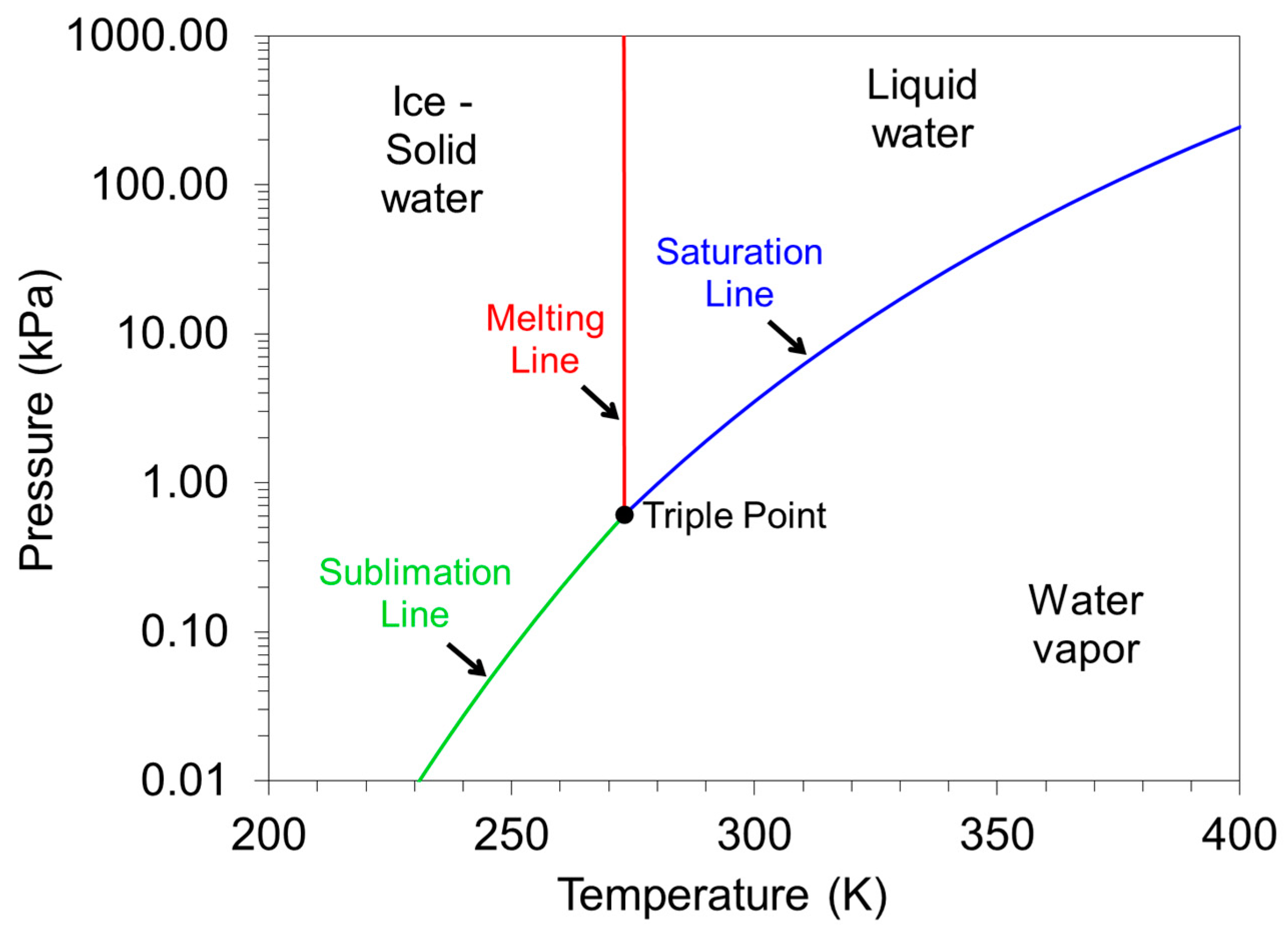
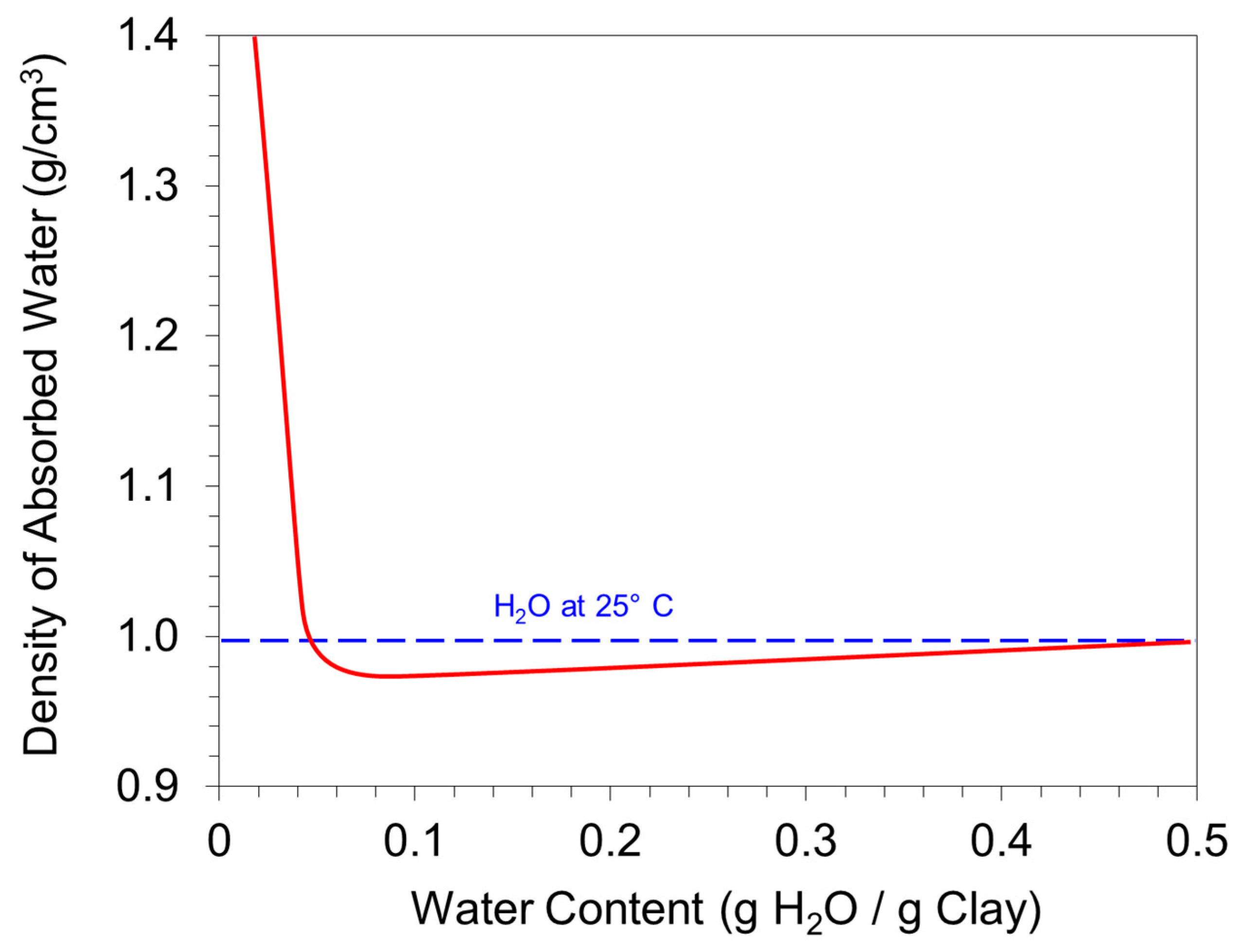
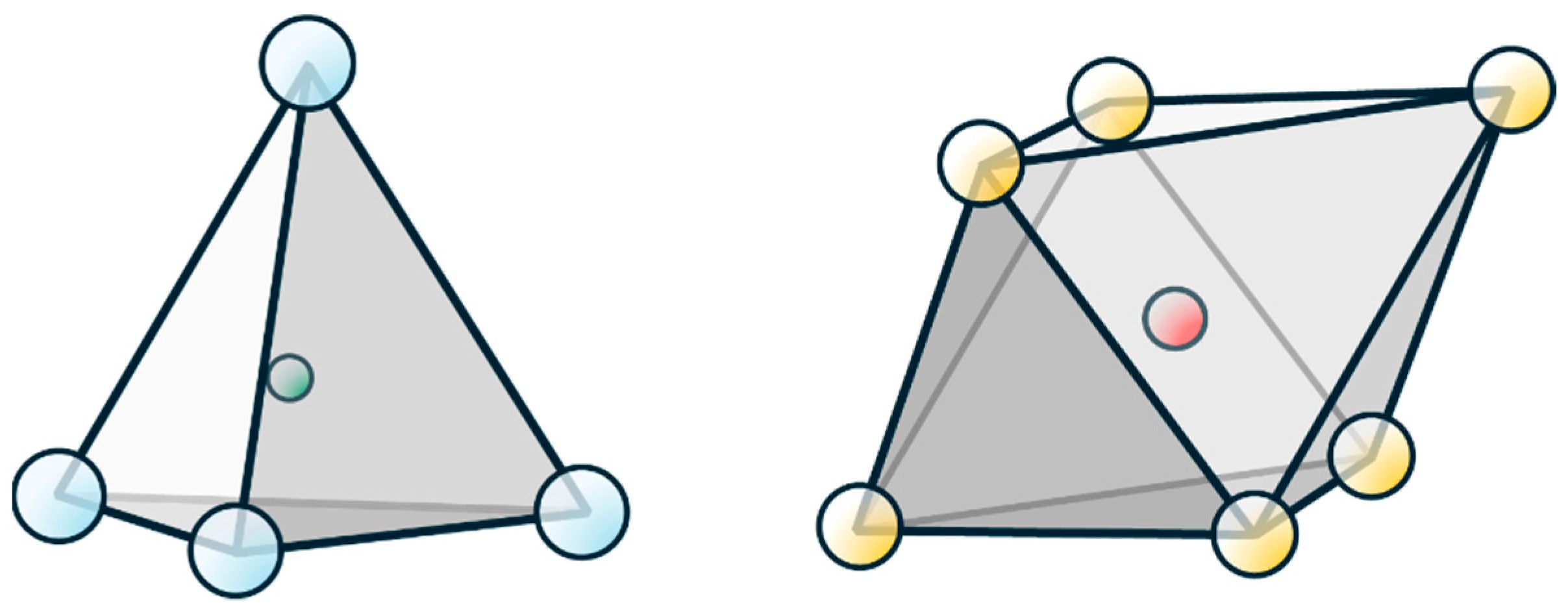
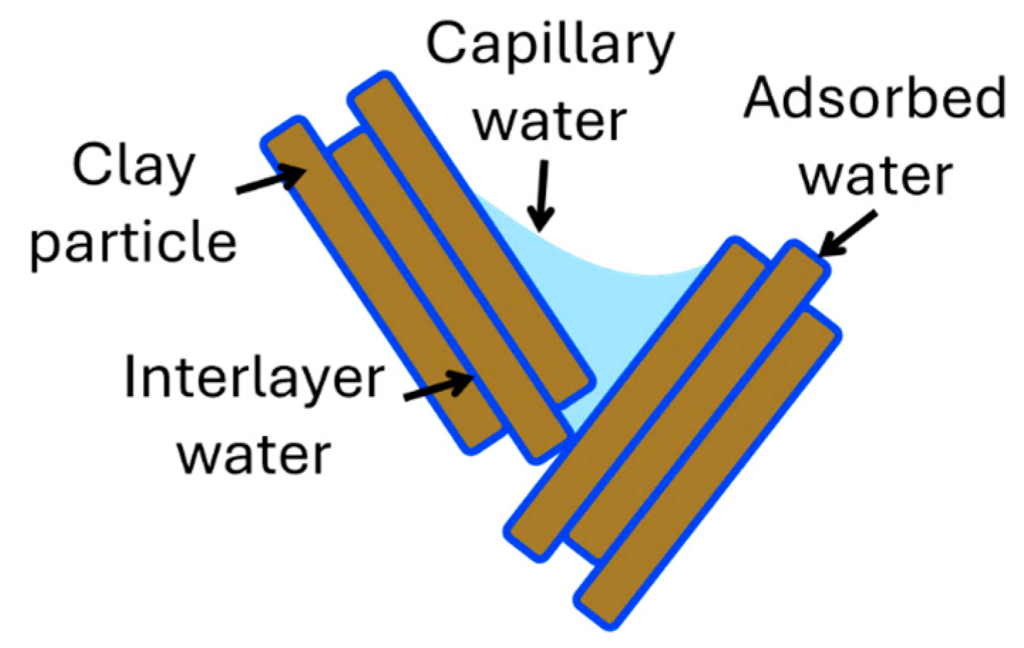
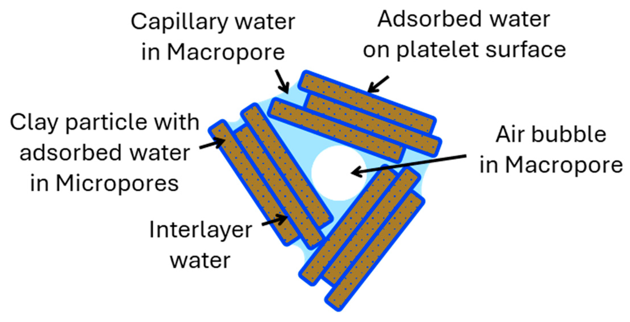

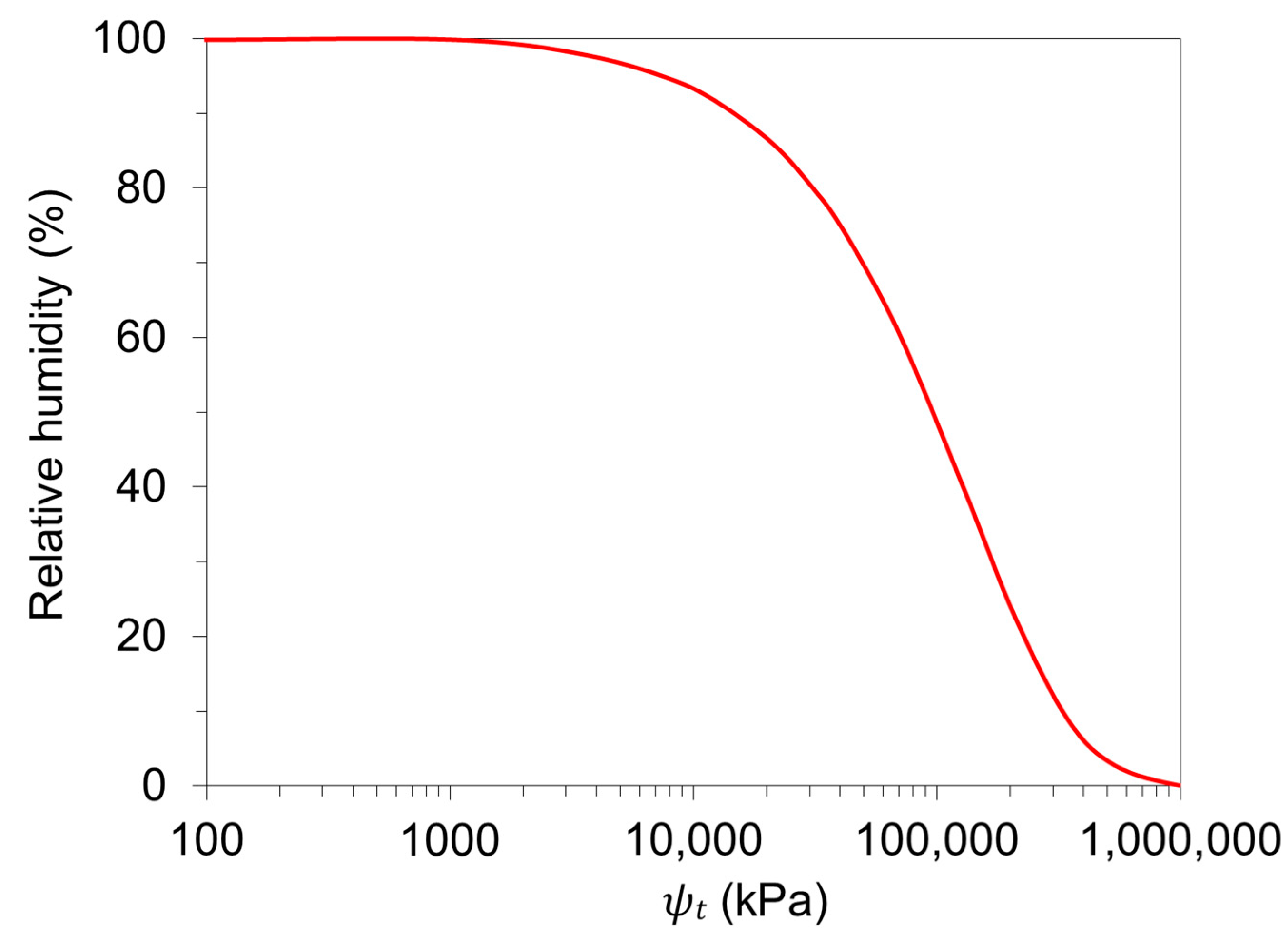
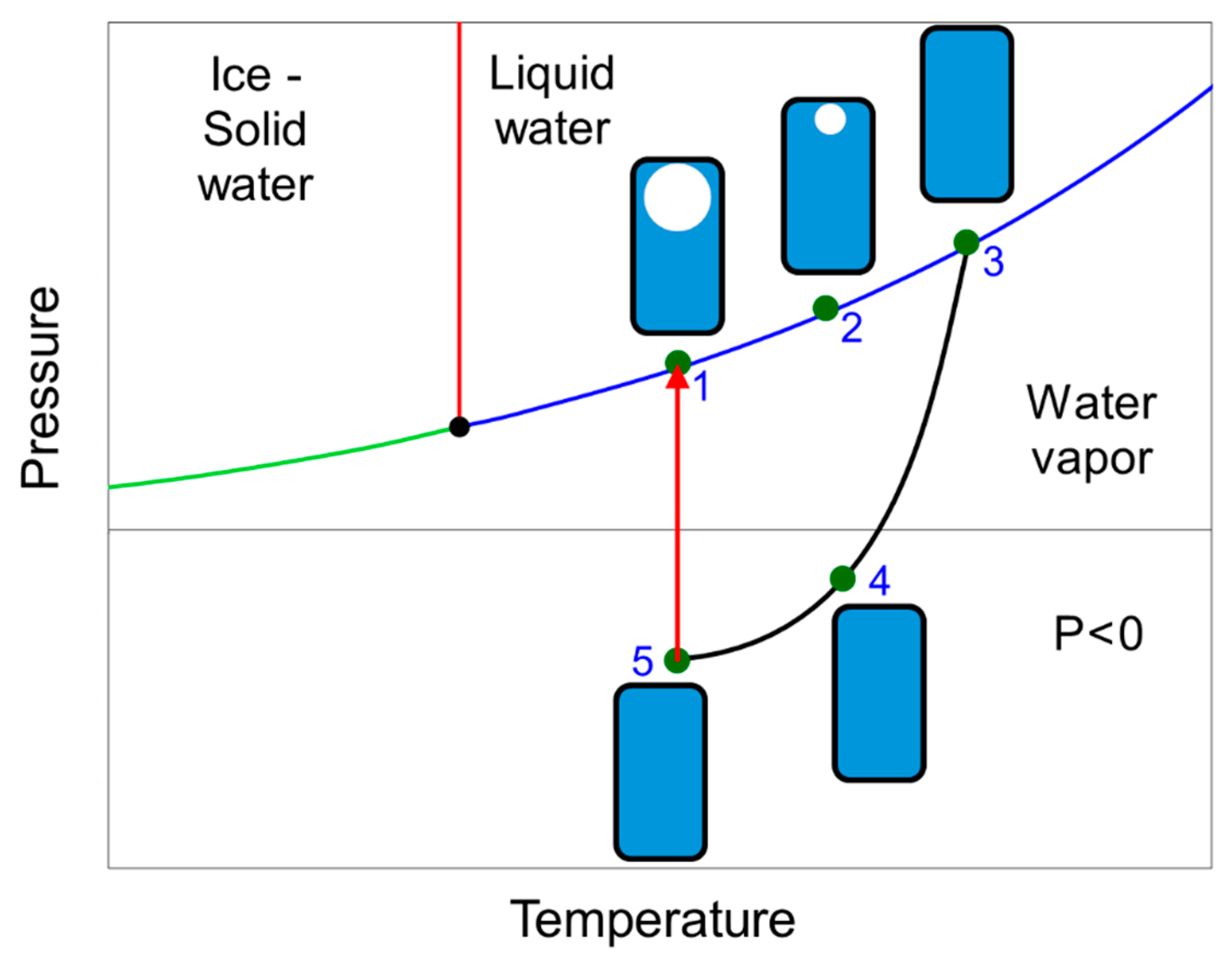
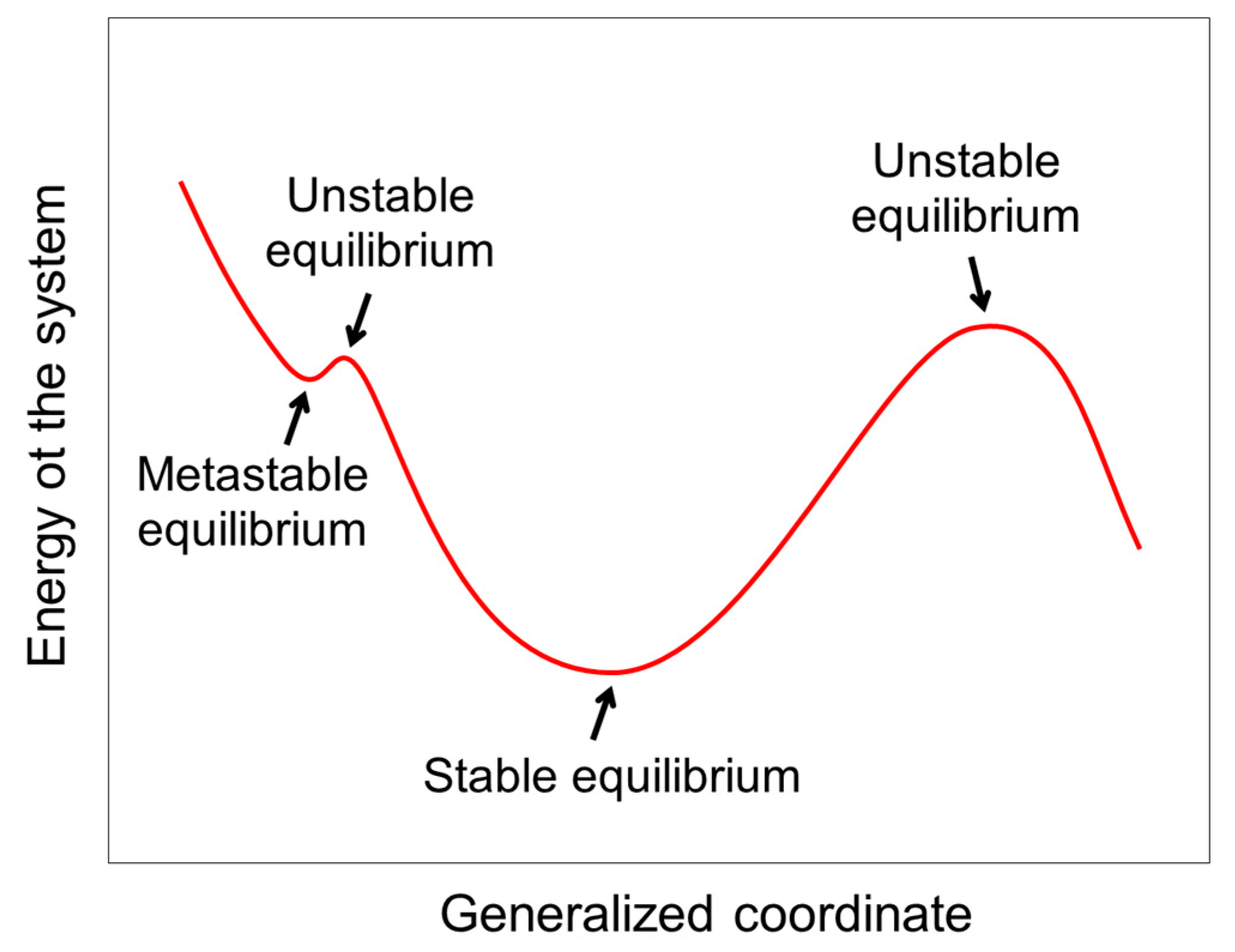
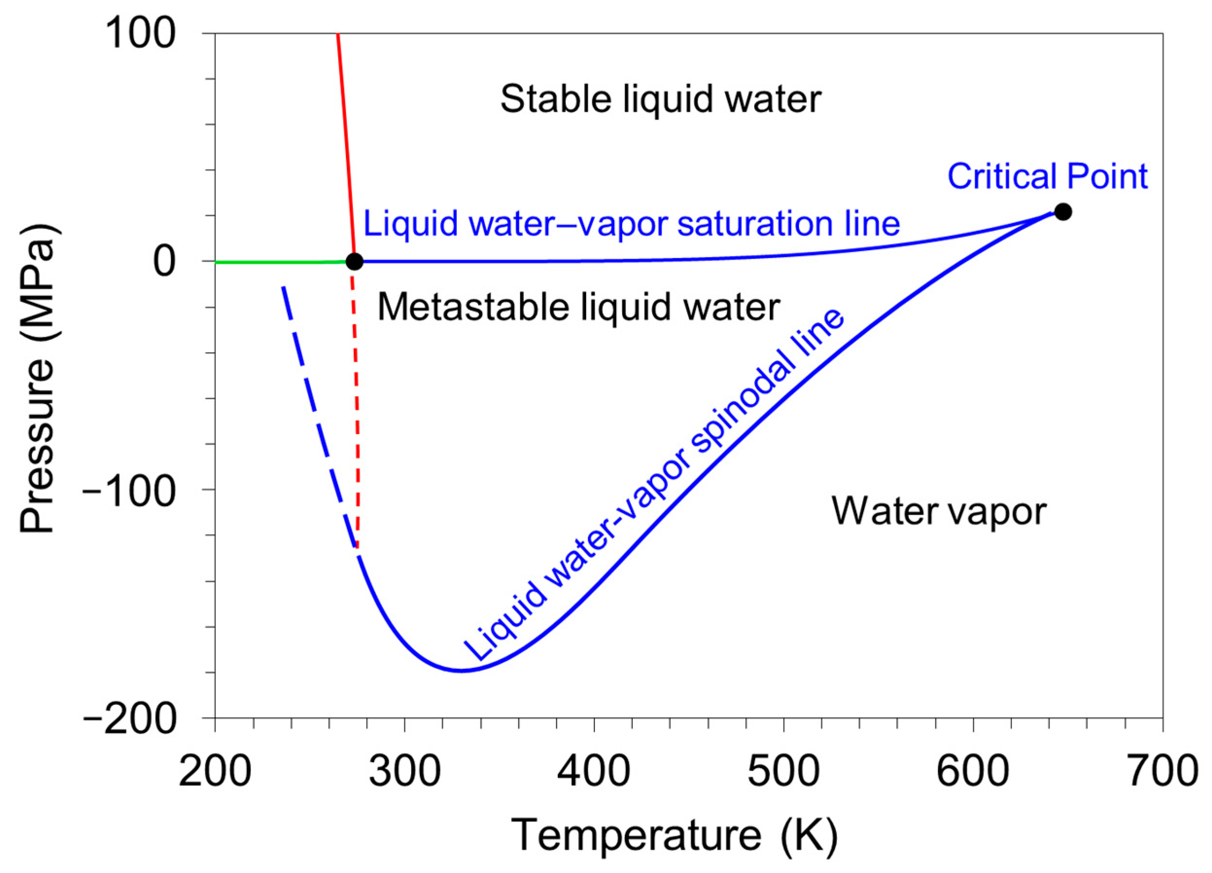
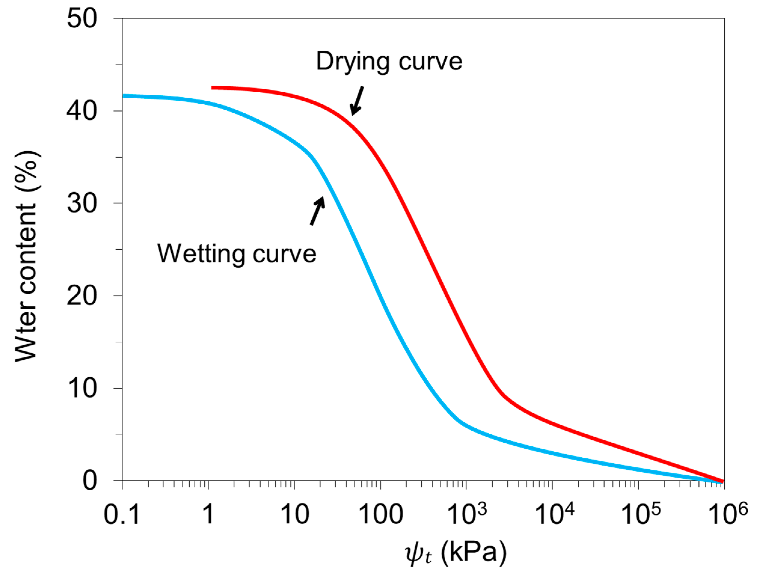

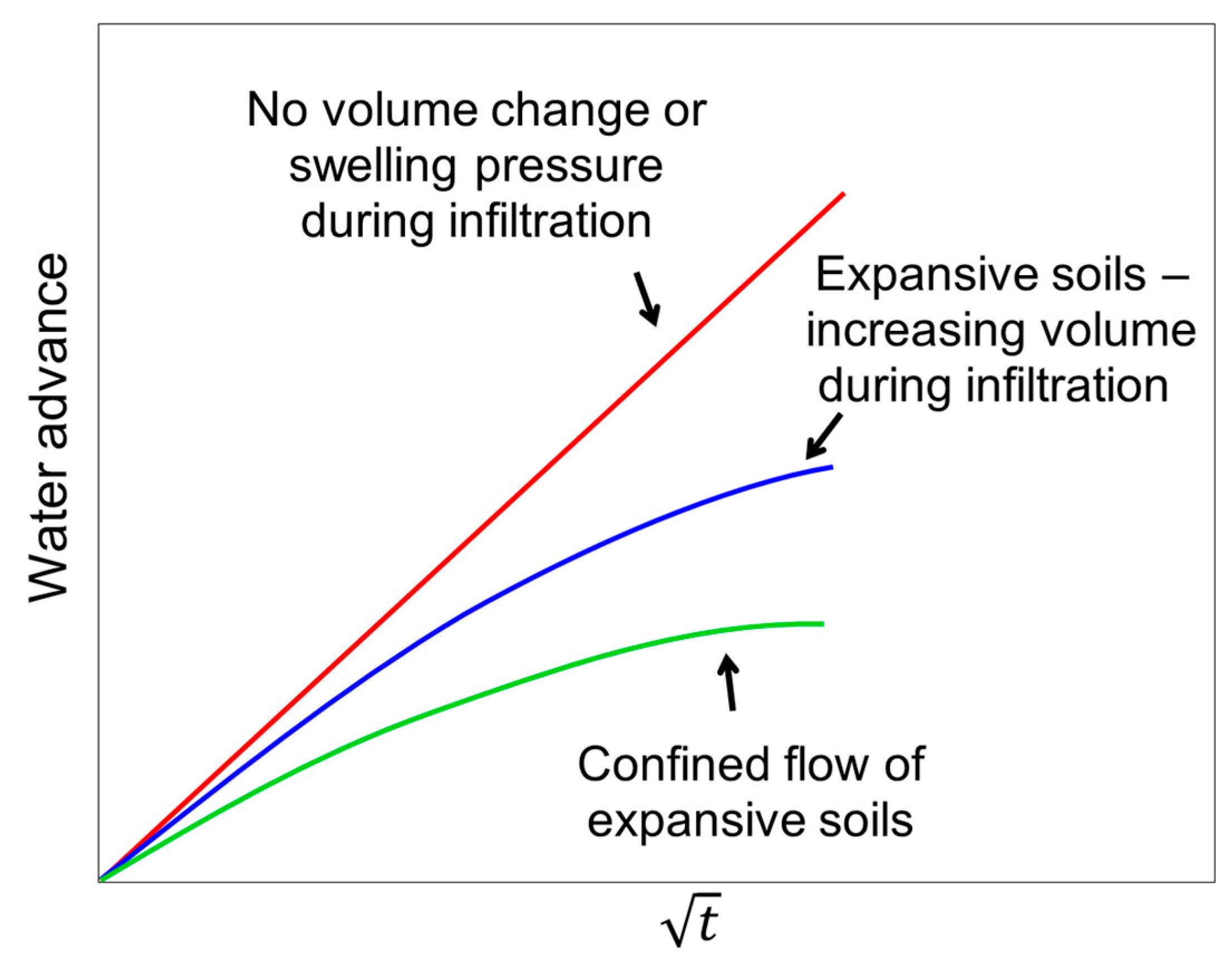
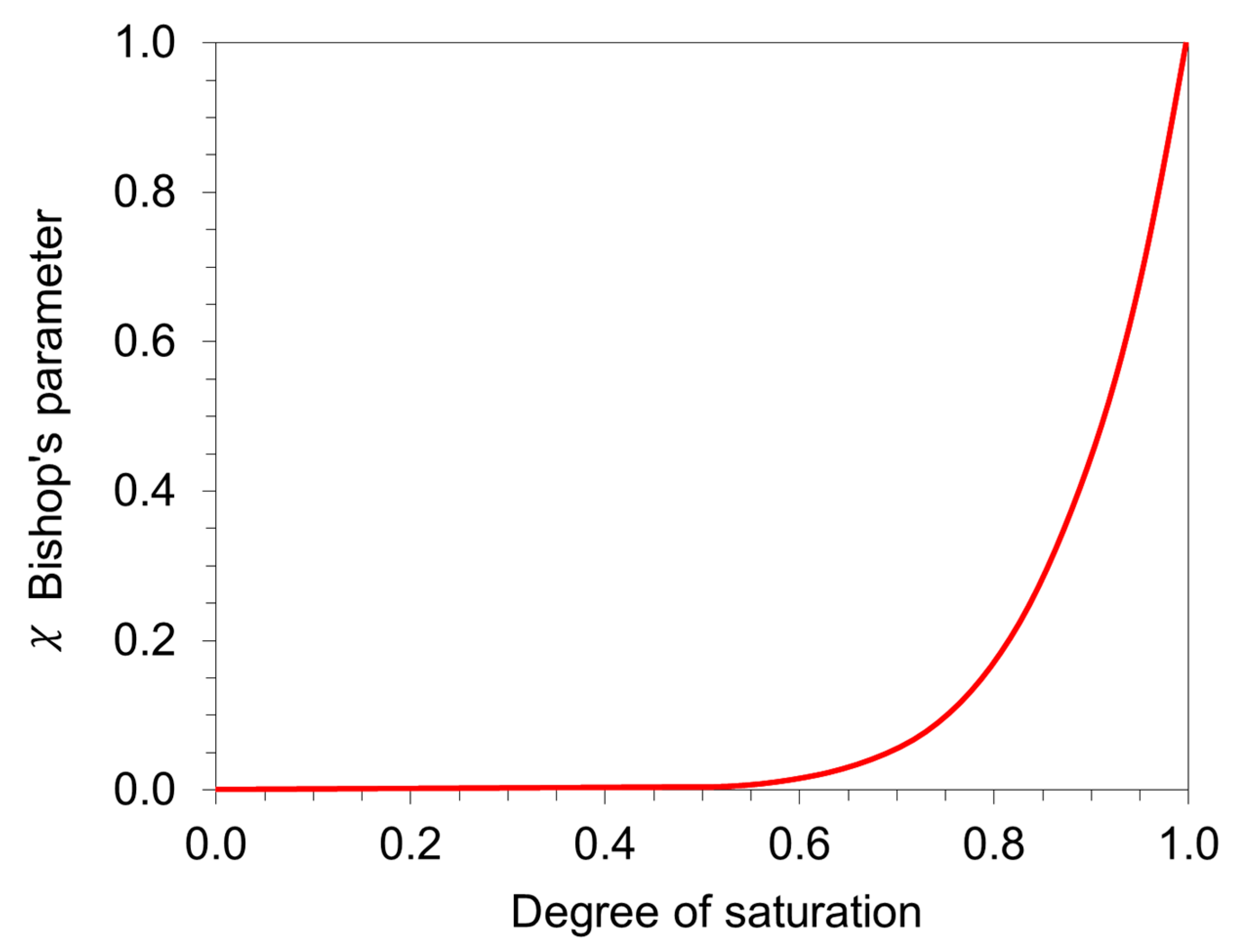
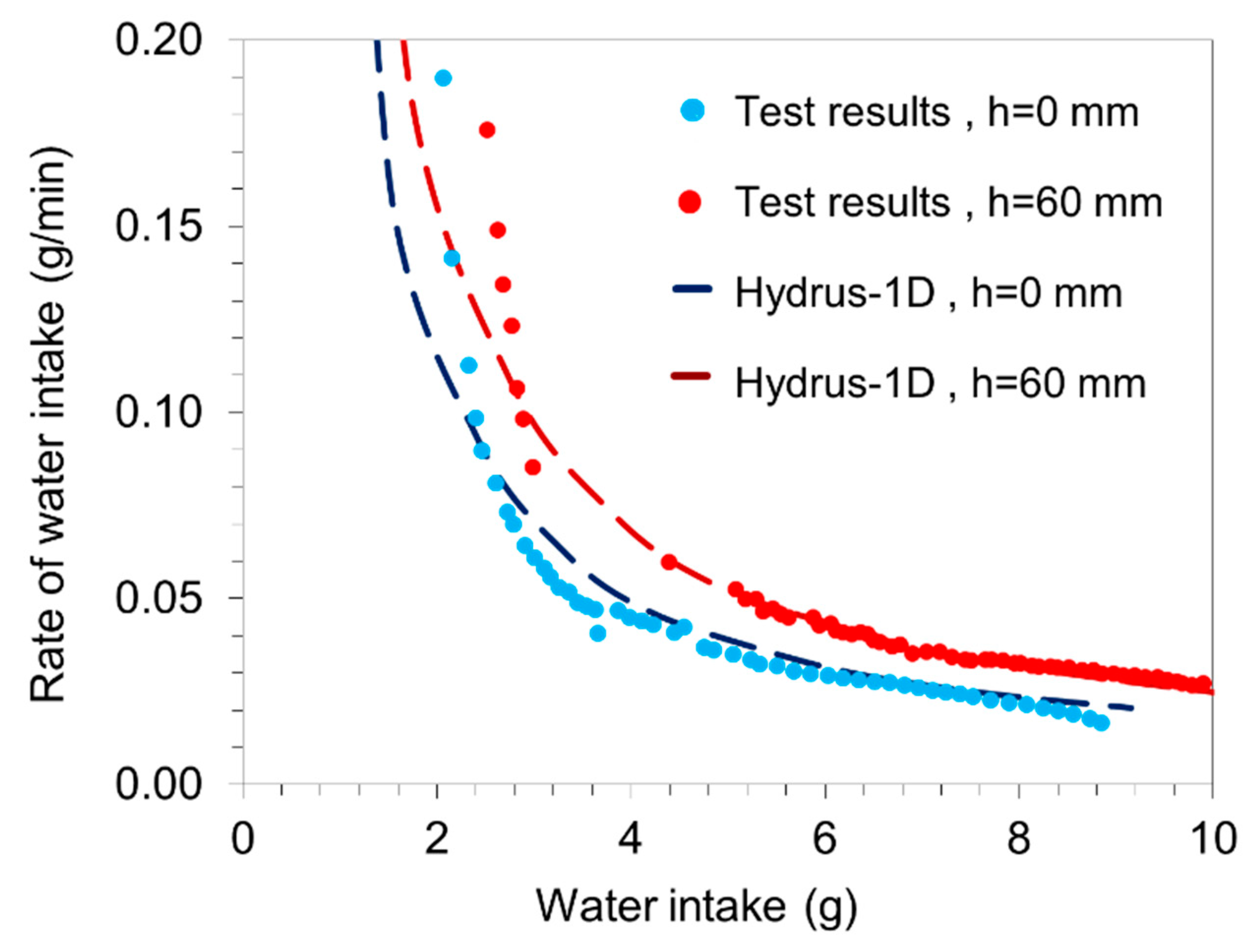
Disclaimer/Publisher’s Note: The statements, opinions and data contained in all publications are solely those of the individual author(s) and contributor(s) and not of MDPI and/or the editor(s). MDPI and/or the editor(s) disclaim responsibility for any injury to people or property resulting from any ideas, methods, instructions or products referred to in the content. |
© 2025 by the author. Licensee MDPI, Basel, Switzerland. This article is an open access article distributed under the terms and conditions of the Creative Commons Attribution (CC BY) license (https://creativecommons.org/licenses/by/4.0/).