Review

A Review of Parameters and Methods for Seismic Site Response

1
Département des Sciences Appliquées, Université du Québec à Chicoutimi, 555 Bd de l’Université, Chicoutimi, QC G7H 2B1, Canada
2
Earth Sciences Department, University of Western Ontario, 1151 Richmond St, London, ON N6A 3K7, Canada
3
Geological Survey of Canada, 490 R. de la Couronne, Québec, QC G1K 9A9, Canada
4
Hydro Québec, 75 Boul. René-Lévesque O, Montréal, QC H2Z 1A4, Canada
*
Author to whom correspondence should be addressed.
Geosciences 2025, 15(4), 128; https://doi.org/10.3390/geosciences15040128
Submission received: 11 December 2024 / Revised: 13 March 2025 / Accepted: 18 March 2025 / Published: 1 April 2025
(This article belongs to the Special Issue Geotechnical Earthquake Engineering and Geohazard Prevention)

Abstract

:
Prediction of the intensity of earthquake-induced motions at the ground surface attracts extensive attention from the geoscience community due to the significant threat it poses to humans and the built environment. Several factors are involved, including earthquake magnitude, epicentral distance, and local soil conditions. The local site effects, such as resonance amplification, topographic focusing, and basin-edge interactions, can significantly influence the amplitude–frequency content and duration of the incoming seismic waves. They are commonly predicted using site effect proxies or applying more sophisticated analytical and numerical models with advanced constitutive stress–strain relationships. The seismic excitation in numerical simulations consists of a set of input ground motions compatible with the seismo-tectonic settings at the studied location and the probability of exceedance of a specific level of ground shaking over a given period. These motions are applied at the base of the considered soil profiles, and their vertical propagation is simulated using linear and nonlinear approaches in time or frequency domains. This paper provides a comprehensive literature review of the major input parameters for site response analyses, evaluates the efficiency of site response proxies, and discusses the significance of accurate modeling approaches for predicting bedrock motion amplification. The important dynamic soil parameters include shear-wave velocity, shear modulus reduction, and damping ratio curves, along with the selection and scaling of earthquake ground motions, the evaluation of site effects through site response proxies, and experimental and numerical analysis, all of which are described in this article.

1. Introduction

Recent strong earthquakes have demonstrated their destructive potential, causing damage to structures and disruption of human activities, e.g., 2010 M8.8 Chile, 2011 M9.0 Tohoku, 2013 M7.7 Pakistan, 2015 M7.8 Nepal, 2018 M7.5 Sulawesi Indonesia, 2021 M7.2 Haiti, 2023 M7.8 Turkey-Syria, etc. Since the 1985 M8.0 Mexico City earthquake, it has been fully recognized that near-surface geological and geotechnical conditions can significantly impact the amplitude–frequency content and duration of the bedrock ground motion [1]. Specifically, when the vertically propagating seismic shear waves encounter a low stiffness medium, their propagation velocity decreases rapidly, whereas the amplitude increases, thus conserving their energy [2]. This phenomenon is commonly referred to as the “site effect”.
In the case of a relatively uniform infinite soil layer on top of considerably stiffer bedrock, the site effect is characterized by a well-defined single amplification peak at the soil fundamental vibration period. A multiple peak amplification corresponds to the presence of multiple heterogeneous surficial layers, whereas broadband amplification occurs when a relatively gradual decrease of the shear-wave velocity (VS) takes place towards the ground surface [3]. In addition to impedance contrasts between surficial layers, amplification of ground shaking may also occur because of topographical conditions and basin effects. Typically, soft soils with low shear-wave velocity (strength) tend to amplify low-frequency bedrock motions from distant earthquakes, while stiff shallow soils amplify the high-frequency content from nearby earthquakes [4]. It was also confirmed that the dynamic response of structures built on soft soils differs from those on stiff soils and rock outcrops, which can lead to increased damage [5]. Whatever the cause of the local amplification, it may contribute to important variations of the ground motion intensity at relatively short distances.
The development of sophisticated analytical and numerical models for predicting potential seismic shaking at the ground surface and consecutive negative impacts on the built environment is rapidly advancing, among which the finite element and finite difference are the most frequently used. They apply advanced constitutive stress–strain models to simulate the soil’s nonlinear dynamic behavior during the cyclic loading of the input ground motion. Accounting for site effects typically involves the development of design ground motions through experimental and numerical methods. Numerical techniques include linear and/or nonlinear seismic response analyses in 1D, 2D, or 3D, requiring representative geotechnical properties and ground motion inputs. To this end, one of the objectives of geotechnical earthquake engineering is to understand, measure, and quantitatively model important soil properties and ground motion parameters [6].
Important soil geotechnical properties include soil density (ρ), small strain shear modulus (Gmax) and the associated shear-wave velocity (VS), shear modulus reduction curve (SM), damping ratio curve (DR) and Poisson’s ratio (ν). The soil mechanical properties and dynamic response vary with cyclic loading and strain levels and, therefore necessitate representative field and laboratory measurements [7]. Various techniques exist for their assessment, each with its pros and cons concerning different parameters and soil types [8]. The advantage of laboratory tests is that they allow control of important settings, such as the confining pressure and dynamic strain. In contrast, field investigations provide measurements under undisturbed conditions and are representative across larger soil volumes. Of interest are also the local site parameters, such as the time-averaged shear-wave velocity of the soil deposits, shear-wave velocity of the top 30 m (VS30), and the fundamental vibration period (T0), which are commonly used as proxies for the prediction of the potential amplification of the bedrock motion.
The intensity of the seismic shaking is typically calculated for reference soil conditions, usually the interface between surficial sediments and bedrock, with VS values ranging from 760 m/s to 3000 m/s [9]. The seismic hazard can be represented through the probability of exceedance (return period) curves for various ground motion parameters, such as spectral accelerations (Sa), peak ground acceleration (PGA), peak ground velocity (PGV), or with a uniform hazard response spectrum across the entire period range of interest. What-if earthquake scenarios are also used to simulate the seismic input. To ensure the reliability of the time domain simulations, suites of hazard-consistent acceleration time histories are needed in this case [10]. This requirement, however, may be a problem in low to moderate seismicity intraplate regions characterized by less frequent earthquakes and an insufficient number of strong-motion records. In such cases, alternative approaches must be applied, including upscaling existing accelerograms, ground motions recorded in regions with similar site conditions, and/or synthetic ground motions [11].
This paper aims to comprehensively review the parameters and methods for evaluating the seismic site response. This includes (i) determination of essential soil parameters for dynamic analysis, (ii) assessment of the seismic hazard and selection of representative ground motions, (iii) evaluation of potential site effects and their relationship to amplification of the ground motion through site effect parameters as well as numerical and experimental analysis. The conclusions provide a critical summary of the present review and highlight the procedures that must be followed to ensure an accurate assessment of the dynamic soil response.

2. Site Effects

Local geological and geotechnical properties of soils can impact the amplitude–frequency content, and duration of the incoming seismic waves [12]. This phenomenon, referred to as the site effect, may lead to significant variations in seismic shaking intensity and associated damage potential at short distances [13]. The most frequent site effects are schematically presented in Figure 1.
As can be observed in Figure 1, the seismic site effect is a complex phenomenon involving a variety of factors, such as impedance contrast at the interface between geological layers (Figure 1a,b), focusing effects due to irregularities in bedrock and terrain topography (Figure 1c), basin-edge effects (Figure 1d), etc. Seismic site effects and soil amplification have been widely studied during past strong earthquakes. The 1985 M8.0 Mexico City earthquake probably helped the engineering community learn the most important lessons. The epicentral distance was about 350 km, the distance traveled by seismic waves through the rock before entering the Mexico City basin. The simplified stratigraphy of the lake zone beneath the downtown area consists of approximately (from the ground surface) 30 m thick of incredibly soft clayey lake sediments and 60 m of stiff clays on top of well compacted and dense sandy silt [14]. The estimated PGA amplification on soft soil was up to 5 times higher than the PGA measured on rock outcrops. The highest amplification of about 8 times occurred in spectral accelerations around 2.0 s, the fundamental vibration period at about 40 m thick, soft lake sediments. The high damage observed in buildings with a vibration period of about 2.0 s (12–20 stories) was attributed to the resonance effect in the soft lake sediments exposed to distant earthquakes with energy content around the same period range. The intense motion duration of the seismic waves trapped in soft lake sediments was elongated to about 60–100 s, comparatively longer than on rocky sites, translating into an increased number of cyclic loadings that would occur otherwise [15,16]. Likewise, Victoria in British Columbia experienced significant soil amplification during the 2001 M6.8 Nisqually earthquake. The strong impedance contrast between the Victoria clay (Vs = 164~262 m/s) and bedrock (Vs = 2000~3500 m/s) resulted in peak spectral accelerations at a period range of 0.2~0.5 s up to six times higher at soil sites compared to bedrock sites [17].
Also, topographical effects were observed during the 1987 Whittier Narrows earthquake in California, contributing to as much as ten times higher amplitudes in a hilly region than in the nearby plains, whereas during the M6.7 Northridge earthquake in 1994, an unexpectedly high PGA = 1.78 was recorded on the same Tarzana Hill, 60-m-tall feature 44 km from the epicenter, which is among the highest PGAs ever recorded [18,19]. The effects of forward directivity in the edge of the epicentral zone were first documented during the Mw 7.3 1992 Landers earthquake and Mw 6.7 1994 Northridge earthquake [20]. High damage concentration observed along the sediment-to-rock boundaries during the M6.7 1994 Northridge and M6.9 1995 Kobe earthquakes demonstrate the significance of the basin-edge effect on ground motion amplification [21,22].
Where possible, the prediction and evaluation of the site effects are based on recorded strong earthquake motions and field observations. The most frequent alternative is to conduct numerical site response analyses using specific dynamic soil parameters and ground motions. This type of analysis evaluates the distribution of soil dynamic stresses and strains exerted by the propagation of the seismic waves and the resulting surface ground motion.

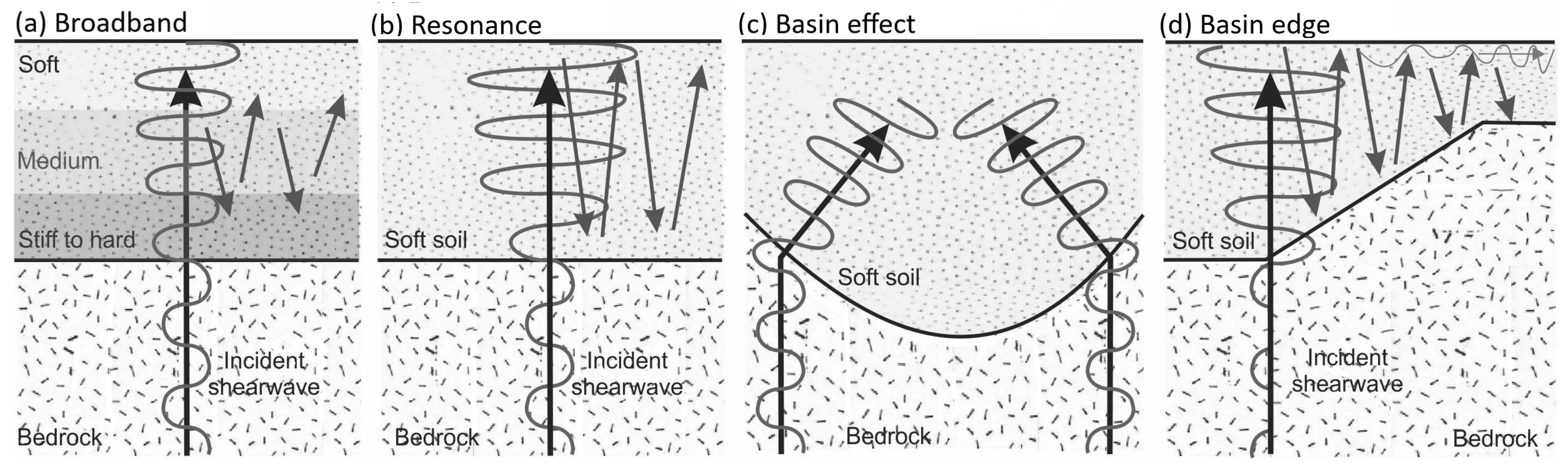
2.1. Resonance Amplification

The amplification of the bedrock motion can be characterized by a single amplification peak at the fundamental vibration period T0 (resonance) of a relatively uniform soft layer with relatively poor mechanical properties on top of stiff soil or bedrock with negligible contribution of other surficial layers; multiple amplification peaks corresponding to a few well-defined surficial layers; and a broadband amplification in case of gradual decrease of Vs towards the ground surface [3]. The resonance amplification is linked to a well-defined strong impedance contrast defined as the ratio between the products of Vs and density in soft and stiff units, ~ρrockVsrock2soilVssoil2. It governs the seismic wave reflection and transmission process. In this case, the vertically propagating horizontal shear-wave amplitude increases as the Vs decreases. They become trapped within the low Vs layer, reflecting back and forth between the ground surface and the soil-bedrock interface at the fundamental vibration period of the soft soil unit. Equation (1) [1] provides the fundamental resonant period (f0) and harmonics (f1, f2, …). The fundamental resonance frequency, f0, is often linked to the most significant spectral peak of the resonance transfer function; the amplitude of this peak varies directly, as in Equation (2).
fn = (Vsavg/4H) × (1 + 2n) for n = 0, 1, 2, 3, 4…….
Ares ~ (ρrock × Vsrock)/(ρavsoil × Vsavsoil)
Here, Vsavg, H, ρavsoil, and Vsavsoil are the average shear-wave velocity of the soil (m/s), the thickness of the soil column (m), the average density of the soil column and travel-time-weighted average shear-wave velocity of the soil column, respectively.
T0 is an essential property and depends on geometrical and mechanical soil properties, T04H/VSsoil, where H is the thickness of the soil layer [1]. The effects of T0 and H have been evaluated and shown to be significant in low-strain linear site amplification [23,24]. Figure 2 depicts the linear amplification vs. the ratio of the vibration period to the natural soil period of different soil models in the Saguenay region of eastern Canada, as derived from a 1D ground response simulation. It reveals that resonance amplification occurs near the natural period of the soil. Recent earthquakes, like the M5.8 Mineral Virginia earthquake in 2011, highlighted the seismic hazards in the region, with VSsoil ~150–200 m/s and VSrock ~2700 m/s, leading to a significant impedance ratio and linear amplitude increase of roughly ≥12 across a broad frequency band.

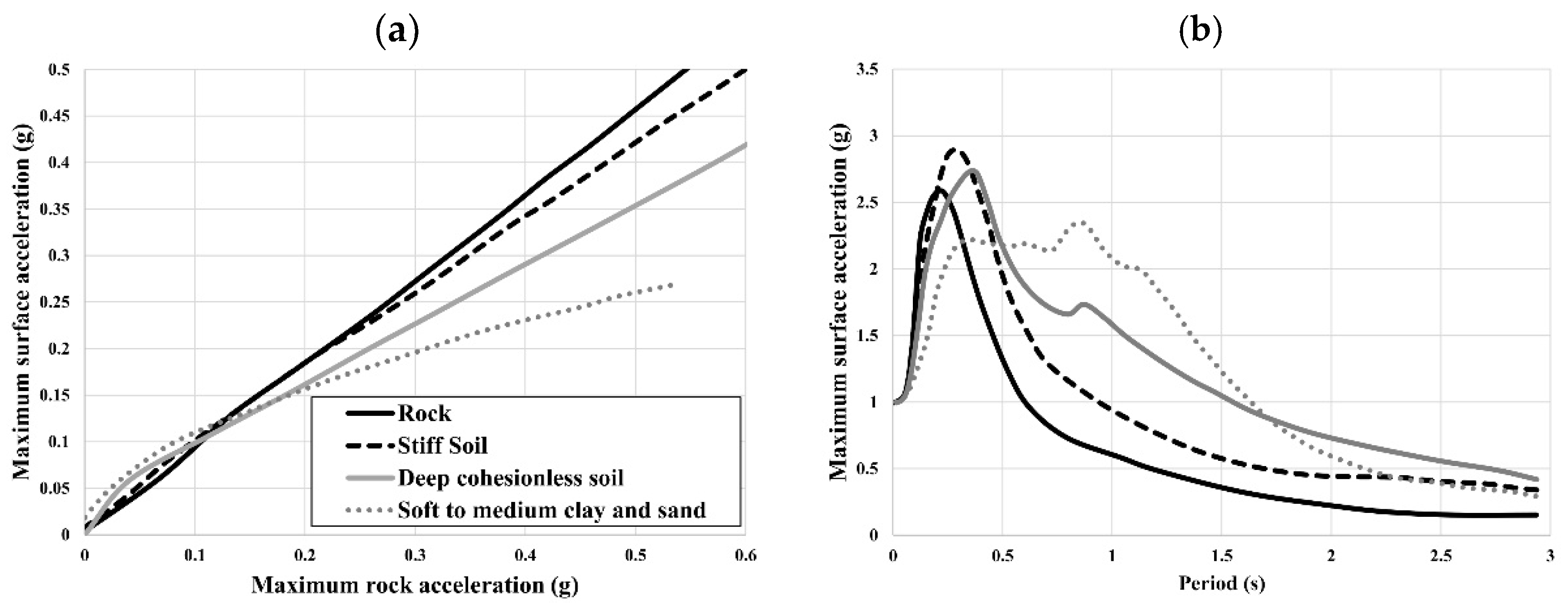
2.2. Broadband Amplification

Broadband amplification often occurs due to the decrease in soil Vs toward the ground surface and the resulting impedance contrast, which shortens earthquake wavelengths and increases shear-wave amplitudes across a broad frequency range (Figure 1a) [2]. The amplification effect is proportional to the square root of the potential impedance contrast at the bedrock interface or within the surficial stratigraphy, as shown in Equation (3).
A ~ (ρrock × Vsrock)/(ρsoil × Vssoil)1/2
Here, ρrock, ρsoil, Vsrock, and Vssoil are, in order, the average bedrock density, the average soil density, the shear-wave velocity of the bedrock at the interface between the overburden and the bedrock, and the shear-wave velocity of the soil at the ground surface.
The Mexico City earthquake provided examples of broadband soil amplification at locations with deep, soft lake sediments [26]. The significant impedance differential between cemented sand and gravel (VS ~500–900 m/s) and lake deposits (VS ~75 m/s) beneath it contributed to damage in Mexico City, with amplification ratios reaching 10 at intervals of around 2 s. Victoria, British Columbia, experienced significant soil amplification after the Nisqually earthquake in 2001 due to impedance in VS profiles, and the brown Victoria clay has lower shear-wave velocity values (~164–262 m/s) than bedrock (~2000–3500 m/s), resulting in peak accelerations up to six times higher at soil sites during intervals of 0.2–0.5 s compared to bedrock sites [17]. As documented by Jackson et al. [27], during the 2015 M 4.7 Vancouver Island Earthquake, significant amplification around the 4–6 Hz range was noted in both locations with thick sediment and along the northern boundary of the Fraser Delta.
Broadband amplification and resonant amplification are both influenced by soil composition, thickness, and impedance contrast, and they can be modeled using 1D site response analysis. However, accurately quantifying their respective contributions is challenging due to geological and near-surface heterogeneities, such as topographic effects, lateral variations in soil properties, and complex subsurface layering [28]. In deep sedimentary basins or Quaternary-Holocene deposits, broadband amplification is more pronounced at longer periods (lower frequencies). For instance, amplification factors of 8 to 16 in the Seattle Basin were observed in the range of 0.2–0.8 Hz, with resonance effects attributed to low-impedance deposits in the upper 550 m of the basin [29].
Figure 3 demonstrates the occurrence of both broadband and resonant amplification resulting from subsurface stratification in the Seattle Basin, Washington State. Resonant amplification occurs due to impedance differences, with peaks dictated by the one-way travel time (T) through the layer, expressed as f = 1/4T (f = frequency) [29]. Thin, superficial layers yield high-frequency resonance, whereas deeper layers produce lower-frequency resonance (Figure 3a). Resonant amplification is dominant in shallow layers and appears as sharp peaks at specific frequencies, while broadband amplification occurs when multiple layers interact, spreading complex amplitude increases and resonant amplification over a wider frequency range (Figure 3b).

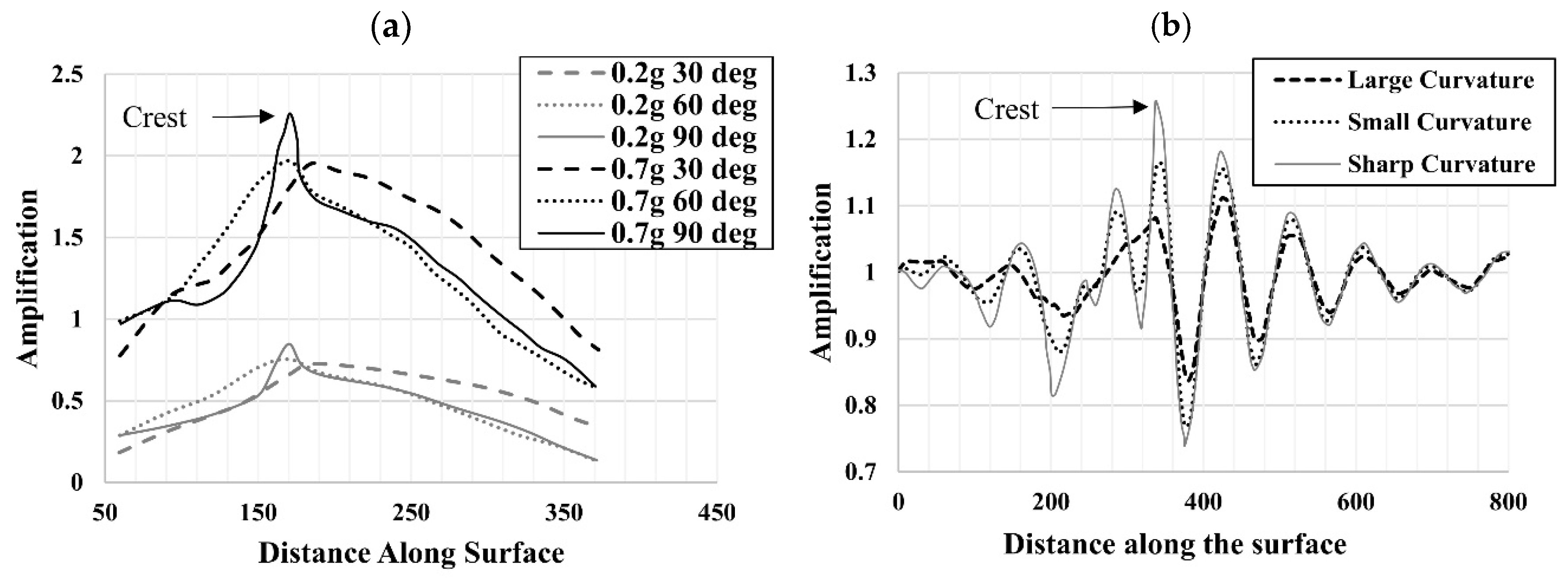
2.3. Topographic Effect
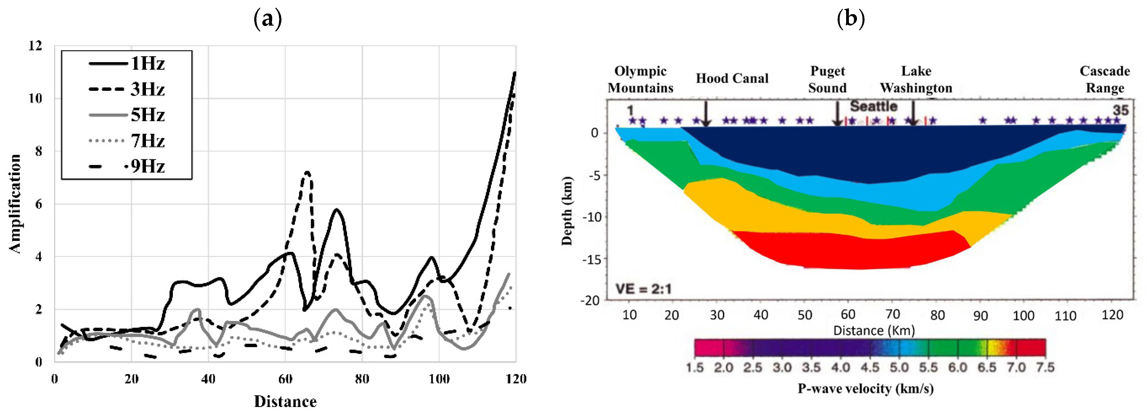
The topographic heights (hills, ridges, etc.) can contribute to the focusing effect on the seismic waves, contributing to an increase in amplitude as opposed to leveled terrains [30]. The increased ground accelerations on topographic highs are caused by seismic waves that enter the topographic ridge’s base, partially reflect into the rock mass, and diffract along the free surface that progressively focuses upward. As one approaches the ridge crest, the constructive interference of these reflections and the corresponding diffractions rises [31]. Topographic lows, such as buried bedrock valleys with a relatively narrow topographic low filled with thick, soft soil sediments, can focus or even diffract seismic waves [32]. The crest of Tarzana Hill, a 60-m-tall feature 44 km from the epicenter, recorded seismic waves during the 1987 Whittier Narrows, California earthquake with an amplitude ten times higher than in the nearby plains [19]. One of the strongest recorded earthquake accelerations, PGA = 1.78 g, was detected on the same hill during the Northridge earthquake in 1994 [18]. Topographic irregularities amplify the acceleration at 2–3 times the slope height (H) from the slope crest [33]. Seismic motion magnifies by up to 70% at the slope’s crest compared to the free field behind the crest [34]. The angle and height of the slope additionally have a significant role in amplification [35]. Slope edge curvature also affects acceleration amplification [36]. The acceleration amplification factor along the surface for slopes with various curvatures is shown in Figure 4.

2.4. Basin Effect

The term “basin-edge effect” describes the reverberation of seismic energy at the wedge-shaped margins, where soft sediments pinch out, and seismic waves trapped in soft sediments deposited in bedrock depressions. As demonstrated in 1909 in Lambesc, France; 1980 in Irpinia, Italy; and 1983 in Liege, Belgium, these diffraction effects are the notable increases in damage intensity that may occur in narrow stiff zones (a few tens of meters) surrounded by softer material [37]. The largest damage, however, was concentrated within an extended zone parallel to both the causative fault and the sediment-to-rock boundary along the Western side of the Osaka basin when the M6.9 Kobe earthquake struck in 1995. The other basin effect considers the impacts of deep sedimentary basins on long-duration ground motions studied in a variety of geographical locations through both numerical simulations [38,39,40,41] and recorded motions [22,42]. Basin effects have been incorporated into the building code for periods T > 1 s, ASCE 7-22, and the USGS National Seismic Hazard Model 2018 [43]. Recently, Kakoty et al. [44] assessed the basin effects of the Georgia sedimentary basin beneath Metro Vancouver. The average basin amplification factors in the deepest locations can reach 2.24 to 6.29 at 2-s intervals compared to basin-edge and outside-basin reference locations. Pratt et al. [29] investigated the Seattle Basin, Washington State, and illustrated that initial body wave arrivals are mainly amplified by 1D basin effects, increasing direct arrivals by 4–6 times at basin sites, while topographic effects contribute only 2–3 times, indicating the dominance of 1D effects beneath the Seattle Basin as shown in Figure 5. It was shown that the amplification was highest at the basin edge.

3. Soil Parameters

3.1. Shear-Wave Velocity (VS)

The Vs (shear-wave velocity) is a key strength parameter directly linked to the elastic shear modulus (Gmax) and is commonly used for calculating soil dynamic response. Vs can be measured or inferred under both field and laboratory conditions. Field tests are categorized into two types: invasive and non-invasive, both of which are also called geophysical tests. The following section provides a general overview of these methods and their advantages and disadvantages.

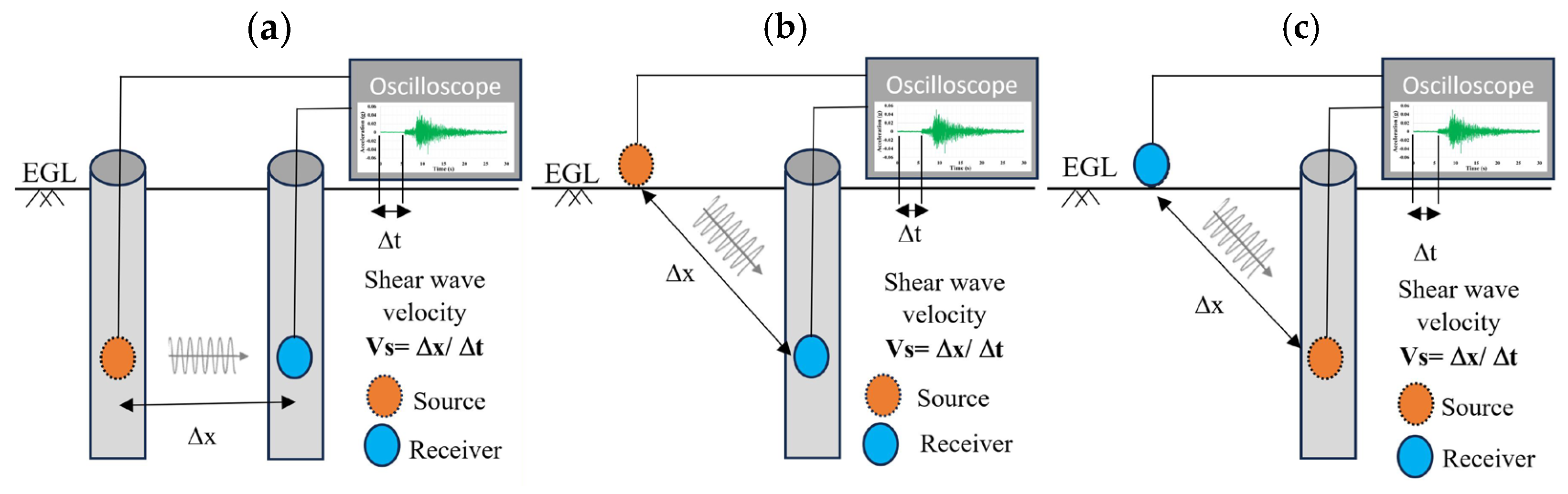
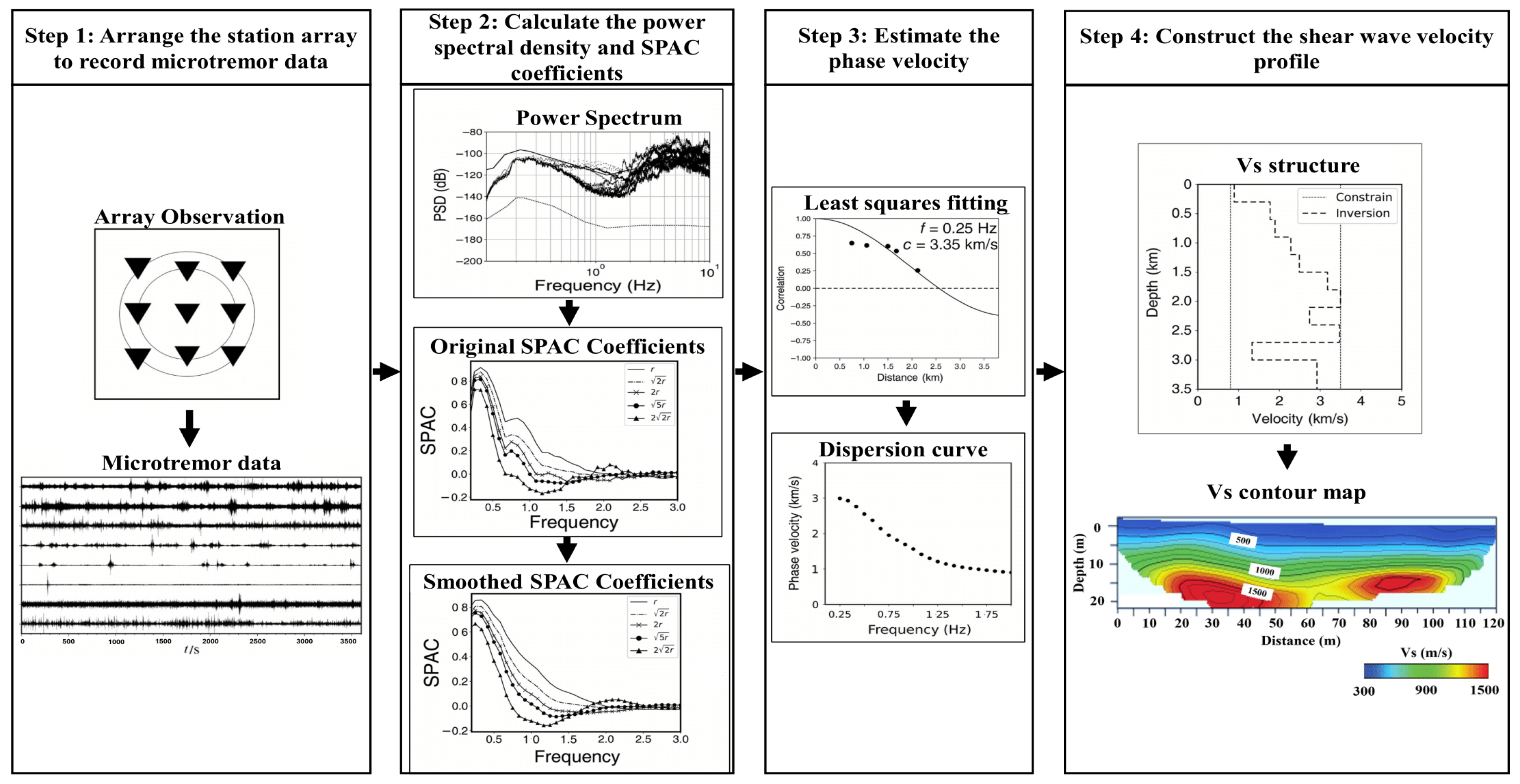
3.1.1. In-Situ Measurements

Invasive in-situ tests, such as the seismic cone penetration test (SCPT) and suspension logging tests, involve the generation of seismic waves (P-wave or S-wave) using methods like sledgehammer strikes, weight drops, or explosives. Suspension logging tests can be categorized into seismic downhole, seismic uphole, and seismic crosshole tests. Figure 6 shows a schematic diagram of a field Vs measurement using a suspension logging test consisting of a geophone receiver and a seismic source to generate waves. To produce a P-wave, a direct vertical impulse is applied to a wooden or steel plank using a hammer, while for S-wave generation, a horizontal blow is applied, and the wave is generated from friction between the soil and the plank [45]. The geophone receiver records the waves in three directions, and the VP and VS are calculated based on the waves’ travel time and distance. These tests provide accurate estimations of wave velocities but can be expensive and somewhat challenging, depending on site conditions.
In SCPT, the seismic downhole test is applied with the CPT. The SCPT enables persistent subsurface assessment and facilitates the development of precise empirical relationships between soil strength properties and Vs [47]. The interpretations of the encountered soil stratigraphy can be based on standard CPTu properties like sleeve friction (fs), cone tip friction (Fr), resistance (qt), friction ratio (Rf = fs/qt), and normalized cone resistance (Qtn). Additional parameters, such as the stress exponent and normalized pore pressure Bq, are used to determine the soil behavior type index Ic. In addition, correlations between CPT data and SPT N-values are often utilized to relate most of the field parameters to SPT N-values. The Vs values are usually inferred from directly measured field parameters, allowing the development of several Vs correlations for different types of soils and depths. Such correlations can be of a regional or site-specific nature, requiring caution when applied to other regions [48]. An extensive list of Vs correlations with CPT parameters is given in Table 1. Table 2 provides the advantages and disadvantages of each method.
Active non-invasive in-situ methods, including seismic reflection and seismic refraction test, are used to measure the compression wave (VP) from the reflected or refracted wave that was generated using a mechanical hammer, and Vs is converted using some empirical correlation from the Vp and other soil properties. However, the seismic refraction test is applicable for thinner subsurface stratigraphy. Other geophysical methods, like Multichannel Analysis of Surface Waves (MASW) or Spectral Analysis of Surface Waves (SASW), rely on generating and measuring surface waves and operate at low strain levels, typically less than 0.001% [60]. Both methods estimate Vs by analyzing the dispersion of surface (Rayleigh) waves, which travel along the Earth’s surface. In MASW, multiple geophones arranged in a linear array record surface-wave propagation across various offsets, creating a dispersion curve that relates phase velocity to frequency. SASW uses only two sensors to measure phase differences at different frequencies to derive the dispersion curve. Vs is calculated by inverting the dispersion curve, fitting observed phase velocities to theoretical models of subsurface properties, and considering factors like layer thickness and Poisson’s ratio. MASW can probe deeper depths and offer better resolution at greater scales, while SASW is more straightforward and more effective for shallow investigations. MASW’s key advantage is its robustness for large-scale surveys and high depth range, but it requires more equipment and computational resources. SASW is cost-effective and easy to deploy but has limited depth penetration and lower resolution for deeper layers.
Passive surface-wave methods based on ambient seismic noise have become essential for measuring shear-wave velocity (Vs) profiles in subsurface investigations. Unlike traditional active seismic techniques, these methods rely on naturally occurring vibrations, such as microtremors caused by traffic, wind, or ocean waves, making them non-invasive and highly suitable for urban and noise-prone areas. By analyzing ambient noise, these methods extract dispersion curves of Rayleigh waves, which are then inverted to derive soil properties. The Spatial Autocorrelation (SPAC) method [61,62,63,64] is a cornerstone of passive techniques. It estimates phase velocities using circular sensor arrays and computes spatial correlations of recorded ambient noise. However, the SPAC method’s limitation in requiring circular arrays led to the development of the Extended SPAC (ESAC) method [65,66,67,68]. ESAC allows irregular sensor configurations, such as L-, T-, or X-shaped arrays, making it more practical for constrained urban environments while maintaining accuracy. The two approaches share a very similar mathematical foundation, and a thorough derivation is available in [61,66,69]. The flowchart of the procedure for the SPAC methodology proposed by Aki 1957 is shown in Figure 7 below.
The Frequency-Wavenumber (FK) method examines the frequency and wavenumber relationship of seismic waves to derive Rayleigh wave dispersion curves [66,70,71,72,73]. Its subtypes, including high-resolution and conventional beamforming methods, have demonstrated broad applicability in resolving subsurface features. Similarly, the Refraction Microtremor (ReMi) method, introduced by Louie [74], uses linear arrays to record ambient noise and applies advanced transformations, such as the τ-p transform, to estimate deeper Vs profiles effectively. Hybrid approaches, such as the Multichannel Analysis of Passive Surface Waves (MAPS), combine SPAC with Multichannel Analysis of Surface Waves (MASW) to overcome azimuthal challenges and enhance subsurface imaging [75,76,77]. These techniques improve the resolution of phase velocity dispersion data, enabling detailed characterization of complex soil and rock structures.
Passive and active seismic methods differ in their data sources and applications. Passive methods rely on ambient noise or natural seismic events, making them cost-effective, less intrusive, and suitable for large-scale studies. In contrast, active methods use controlled sources, offering higher resolution and precision but at a more significant cost and environmental impact. Passive methods have advantages such as minimal fieldwork, lower costs, and the ability to explore deeper subsurface layers, making them valuable for geotechnical investigations, seismic hazard assessments, and infrastructure monitoring. However, their effectiveness depends on ambient noise quality, with limitations in depth resolution for very deep layers, challenges in array configurations, and high computational demands. Despite these drawbacks, advancements in passive techniques have enhanced their accuracy and practicality, solidifying their role in modern geophysics.

3.1.2. Laboratory Measurements

Non-invasive laboratory tests determine Vs from undisturbed soil samples, categorized into (i) low-strain methods such as resonant column, ultrasonic pulse test, piezoelectric bender element test, and (ii) high-strain tests like the cyclic triaxial test, cyclic direct simple shear test, and cyclic torsional shear test. In these tests, a seismic pulse is applied to the soil sample, and Gmax is estimated as Gmax = ρVs2, where ρ represents soil density. Direct use of Gmax for deformation analysis is not recommended; instead, SM and DR curves as functions of attained strain are applied [78]. Shaking table tests [79] and centrifuge modeling tests [80] are two model test types under controlled laboratory conditions measuring seismic behavior and wave propagation in soil samples. Model tests typically involve cyclic loading on a small-scale physical model, aiding in better seismic simulation and validation of prediction hypotheses. Due to the need for sophisticated equipment and highly trained operators, model testing is usually conducted by academic and governmental organizations.
Low-strain methods, including the resonant column test, ultrasonic pulse test, and piezoelectric bender element test, effectively measure soil properties such as shear modulus and shear-wave velocity at minimal strains. These methods are highlighted on the left side of Figure 8, where the orange region corresponds to the “Very Small Strain” range, typically below 0.001% shear strain. The normalized stiffness ratio (G/Gmax) remains close to 1 at these strain levels, indicating minimal stiffness degradation. As strain levels increase, soil stiffness begins to degrade progressively. The normalized stiffness degradation curve in Figure 8 illustrates this behavior, with the green and blue regions corresponding to the “Small Strain” and “Large Strain” ranges, respectively. These ranges align with geotechnical applications, such as retaining walls, foundations, and tunnels. In the small strain range (0.001% to 0.1% shear strain), stiffness degradation is moderate, making this range critical for foundations and retaining wall analyses. Significant stiffness reduction occurs at more enormous strains (beyond 0.1%), as shown by the steep decline in G/Gmax, which is important for studying slope stability, flow failure, nonlinear site response, and other high-strain applications. High-strain methods, such as the Cyclic Triaxial Test and Cyclic Direct Simple Shear Test, are represented on the right side of Figure 7, where the blue region indicates large strains. These tests capture the nonlinear behavior of soils under cyclic loading and provide insights into deformation, strength, and liquefaction potential. Using normalized stiffness degradation curves from various laboratory tests, as depicted in Figure 8, enables a comprehensive understanding of soil behavior across different strain ranges, making it a crucial tool for evaluating site effects and designing resilient geotechnical structures.

3.2. Shear Modulus and Damping Ratio

Soft soils typically exhibit nonlinear behavior during close strong earthquakes, where an increase in the shear strain leads to a rapid decrease of the shear modulus (SM) and an increase in the material damping ratio (DR) [82]. Such nonlinear behavior is implemented in dynamic soil analysis of ground response or slope stability studies. Seismological evidence from Port Island following the 1995 M6.9 Kobe earthquake highlights significant nonlinearities, particularly the near-perfect filtering of high-frequency motion in a liquefied sand layer [83]. The SM and DR curves must be used to determine the soil’s nonlinear behavior. The following sections describe the measurements and the factors affecting SM and DR.

3.2.1. Measurement of SM and DR

The shear modulus (SM) and damping ratio (DR) vs. strain curves (Gγ and ξγ) are commonly obtained with standard laboratory tests, such as Bender Element, Resonant Column, Cyclic Triaxial Test, Torsional Shear Tests, or Monotonic Triaxial Tests [1]. In those laboratory tests, soil behavior remains nonlinear across a broad range of strain amplitudes, forming a distinct stress–strain route known as the hysteresis loop. A full stress reversal occurs during cycles between equal positive and negative values in the stress–strain relationship loop, which is described with the hysteresis damping ratio (DR) and the shear modulus (G) determined as the slope of a line connecting endpoints (Figure 9).
The area the loop covers measures the soil’s internal damping, representing the energy absorbed during deformation. The soil exhibits the characteristics of a linear elastic material at small strain amplitudes (<0.0001%) with minimal energy loss and maximal shear modulus (Gmax). However, as strength amplitude starts to increase, the shear modulus (G) decreases, accompanied by an increase in the hysteretic damping. The Poisson’s ratio correlates the shear modulus to elastic modules like Young’s (E) and Bulk modulus (K). The factors influencing the strain modulus, damping ratio, and strain amplitude are the number of strain reversal cycles, loading frequency and history, void ratio, relative density, and plasticity index. Grain size distribution and particle surface texture have a lesser impact on the outcomes [6].
While the hysteresis damping ratio (DR) can be measured accurately in a laboratory, its accurate field assessment poses a significant challenge. The seismic piezocone SCPTu and seismic dilatometer SDMT measure two different points on the stress–strain curve, capturing failure states aligned with material strength characteristics and non-destructive attributes related to elastic wave propagation and soil stiffness, E or G [84]. SCPTu and SDMT tests assess stiffness across stress–strain-strength responses utilizing a modified hyperbola [85] to degrade initial stiffness (E0) with increasing load levels and obtain nonlinear load-displacement capacity (Figure 10). Standard procedures for clean sands involve drained penetration with assumed zero effective cohesion intercept (cr = 0) and with a focus on the effective stress friction angle (Nr). In contrast, typical assumptions for clayey soil are total stress assessments with no volume change and penetration data that provide undrained shear strength (cu or su). Various factors, including starting stress state (Ko), anisotropy, boundary conditions, strain rate, loading direction, degree of disturbance, etc., significantly impact the undrained strength.

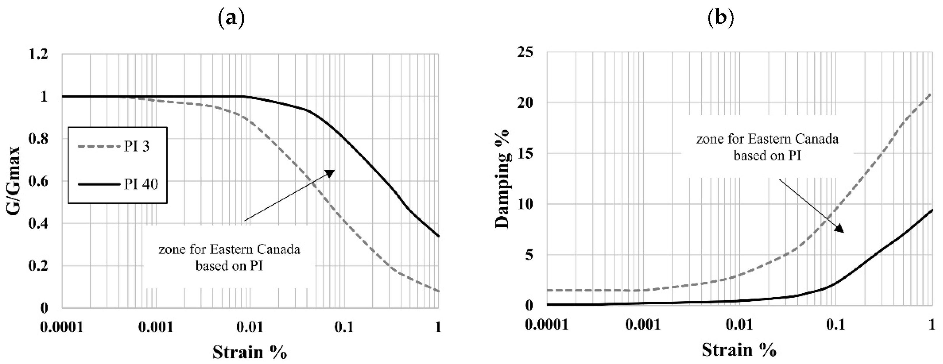
3.2.2. Factors Affecting Shear Modulus Reduction and Damping Ratio Curves

The multiple factors that affect the nonlinear soil behavior are discussed hereafter.

Cohesionless Soil

Numerous studies have confirmed the significant impact of particle grain size, shape, and acceptable particle percentage on the structure of SM and DR curves in coarse-grained soils. Baghbani et al. [86] demonstrated that the roundness, sphericity, and regularity of sand particles during cyclic loading affect the DR, leading to increased DR as particles become more rounded. Saathoff and Achmus [87] highlighted that grain size distribution and shape influence soil behavior, where smaller grains display higher shear strain thresholds and stress-dependent behavior. Parameters such as density, effective stress, percentage of fine particles, confining stress, and moisture content were identified as important, with cyclic shear strain and effective stress being the most critical [88]. Figure 11 illustrates the nonlinear SM and DR relationships with increasing shear strain. At the same time, the increasing vertical stress has an opposite impact on SM and DR, i.e., SM increases while DR decreases [89,90,91].
In cohesionless soils, density and confining stress are important factors affecting SM and DR curves. Rollins et al. [92] and Rohilla et al. [93] highlighted trends related to relative density, effective stress, and loading frequency, indicating that higher strain levels reduce the influence of relative density and confining pressure on the increasing trend of SM and decreasing trend of DR. Bozyigit et al. [94] identified that relative density and void ratio control the dynamic SM of non-plastic sand and low plastic silts, with confining pressure and mean effective stress impacting the dynamic shear modulus. For sand-gravel mixtures, Bayat et al. [95] reported changes in both parameters with an increase in confining pressure, showing an increase in SM and a decrease in DR.

Cohesive Soil

Among the parameters identified to impact the SM and DR in cohesive soils are the geological age, confining pressure, void ratio, cementation, plasticity index (PI), and confining pressure [6,96]. Vucetic et al. [97] determined the plasticity index (PI) as the main factor, and their SM and DR developed for various PI scenarios are frequently used to assess the dynamic behavior of cohesive soils, Figure 12. It was also shown that in cases with decreasing SM, the effective vertical stress and over-consolidation ratio (OCR) has more influence than PI [98]. As an update to earlier work by Seed et al. [88] and Vucetic et al. [97], Darendeli et al. [99] developed SM and DR versus shear strain relations running uncertainty analysis based on PI and effective vertical stress and obtained similar soil type and loading conditions effects.

Sensitive Clay

Sensitive clays represent a special category of fine glaciomarine sediments where the original sea pore water was wholly or partially replaced by the infiltration of fresh atmospheric or groundwater [100]. They are characterized by sensitivity, determined by the ratio of the undisturbed shear strength to the disturbed (remolded) strength of >30. Areas with sensitive clays are frequently found in eastern Canada and Scandinavian countries. The SM and DR curves in sensitive clays appear to be influenced by similar factors. For example, Abdellaziz et al. [101] developed SM and DR versus shear strain relationships for typical eastern Canadian sensitive clays. They compared them with the SM and DR of Vucetic et al. [97] and Darendeli et al. [99]. The results indicate that SM and DR versus shear strain relations for sensitive clays initially follow the trend of conventional clay curves for up to a particular strain level: 0.2% to 0.3% before deviating at higher strains. Figure 13 illustrates the SM and DR curves for sensitive clays in eastern Canada.

3.2.3. Nonlinear Effects in Dynamic Loading

Soft soils generally experience higher amplification under seismic loading due to the low Vs, where an increase in the motion amplitude results in reduced shear strength and increased shear strain. At the same time, due to the nonlinear effect, material damping increases, absorbing more energy and decreasing the motion amplitude. Consequently, the relative amplification may decrease in the case of strong earthquake shaking, a phenomenon addressed by Seed et al. [12] as shown in Figure 14 and supported by numerical simulations [102]. Stiff-soil sites exhibit a quasi-linear behavior for PGA ranging from 0.006 g to 0.43 g [103]. Field observations and calculations suggest that significant nonlinear effects in soft, sandy soils may occur when the PGA at the rock interface exceeds a threshold level of around 0.1 to 0.2 g [37].

4. Seismic Parameters
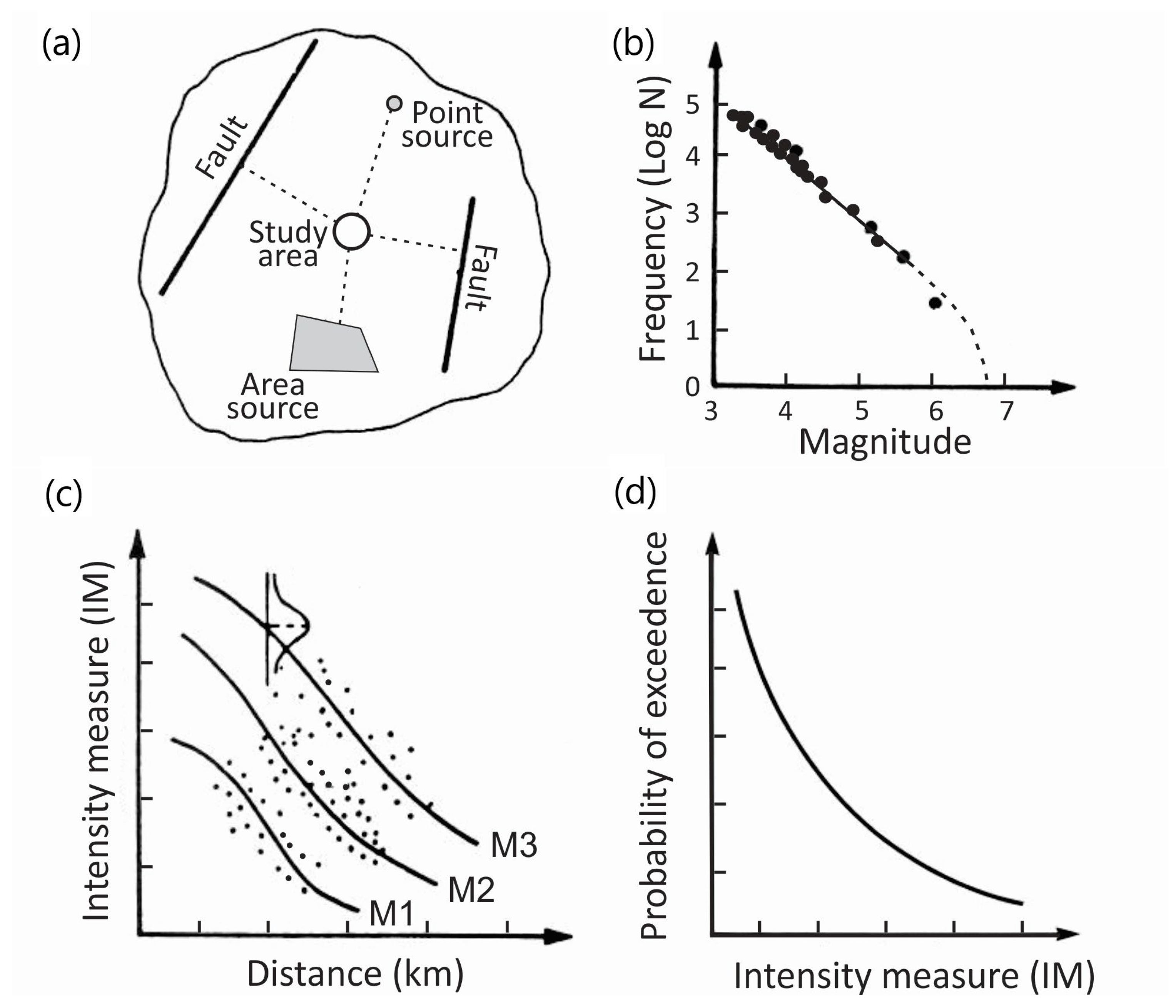
Unlike static analyses, the seismic excitation in dynamic analyses is specified in real or synthetic acceleration time histories. Selecting representative ground motions is an important step relying on criteria such as seismic settings, scaling, and several ground motions required for meaningful analyses. The ground motions are usually selected according to the seismic settings and hazard evaluated for reference site conditions, mainly engineering bedrock with Vs ≥ 760 m/s. The preferred technique for scaling the selected accelerograms is to approximately match a corresponding target response spectrum or to satisfy a specified design level, usually for PGA and/or a spectral acceleration for a given period, Sa(T).

4.1. Seismic Hazard

Seismic hazard represents the likelihood that a potential earthquake with a given intensity will occur in a particular area in a given future period. There are two basic types of seismic hazard analysis: probabilistic (PSHA) and deterministic (DSHA) seismic hazard analysis. PSHA aims to establish the ‘ground motion hazard curve’, indicating the probability of exceeding a specific intensity measure (IM) in the study area. The first step involves identifying active seismic sources and determining their distances from the study area, utilizing point, fault, and areal sources in the source model (Figure 15a). The second step assesses the annual probability of earthquake magnitudes occurring on nearby sources, employing the Gutenberg-Richter relationship (Figure 15b). The third step predicts the intensity of shaking through regression analysis and ground motion models, represented by ground motion prediction equations (GMPEs) [105,106] (Figure 15c). Due to seismic wave complexity and local site amplification, observed data exhibit variation around the median line. The ground motion hazard curve combines the frequency-magnitude model with GMPEs, yielding one point on the elastic spectrum for a given return period (Figure 15d). The process continues for different vibration periods, forming a uniform hazard spectrum (UHS), where each point shares the same probability of exceedance. Typically, the focus is on high-intensity (low-frequency) earthquakes, with the UHS’s high-frequency content influenced by small nearby earthquakes and more extended periods by large distant earthquakes.
The DSHA, on the other hand, provides a relatively straightforward and trackable method for computing the seismic hazard. It calculates the possibility of an earthquake taking place and not its probability. It combines steps (a) and (c) in Figure 15 to generate a single maximum credible earthquake scenario. This is the most severe earthquake scenario expected at a site that gives the most considerable predicted ground motion without explicitly considering the likelihood. For less important projects, the seismic hazard in terms of UHS with a return period of 2475 years (0.000404 p.a.) is prescribed in the seismic design provisions of NBCC 2020 (NRC 2020). UHS for return periods ranging from 98 to 2475 years with local site conditions as a continual function of the time-average shear-wave velocity of the top 30 m (VS30) can be downloaded from the earthquakescanada.nrcan.gc.ca website. The latest 6th generation seismic hazard model of Canada developed within the OpenQuake-engine can be obtained through the same website. It incorporates regional seismic sources with respective maximum magnitudes, earthquake rate data, and epistemic uncertainty in median hazard estimates [9].

4.2. Input Ground Motions

4.2.1. Selection of Real Accelerogram

Representative ground motion records play a crucial role in time domain dynamic analyses. Various regional databases, including the USGS Earthquake catalog, British Geological Survey database, COSMOS, K-NET, KiK-net, NIED, and PEER, store diverse data for earthquakes that have occurred. The ground motion selection process considers earthquake magnitude, source-site distance, local site conditions, and rupture mechanism [107,108]. The selected records must also meet design spectral accelerations with a reasonable scaling factor while maintaining the intense motion duration and waveforms.
The above selection process based on several criteria reduces the pool of candidate records, impacting the reliability of the dynamic analyses [107,109]. The selection of an acceptable number of earthquakes is particularly challenging. Dynamic analyses necessitate acceptable ground motion records, often characterized by the highest response among three inputs to accelerograms or the mean of seven (BSSC 2001; ASCE, 2005a; NERHP 2011). In NBCC 2005, eleven ground motion time histories were proposed, whereas [10] suggested two suites of at least five to six motions for two magnitude-distance (M-R) scenarios. On the other hand, to obtain an average response at a site, Talukder et al. [110] recommend seven records. As can be seen, the minimum number of the sample varies between three and eleven. However, all the above references recommend increased acceleration time histories, mainly when the statistical significance of the uncertainty is evaluated. When the initial selection criteria cannot be satisfied, which is often the case in intraplate regions due to fewer strong earthquakes compared to interplate boundaries, the remaining option is to use increased scaling factors or synthetic ground motions [111]. An exhaustive review of ground motion selection has been illustrated in [112,113,114].

4.2.2. Synthetic Accelerograms

Synthetic acceleration time histories can be generated by simulating the fault rupture mechanism, source-to-site seismic wave propagation, and local site amplification. In this way, a variety of earthquake-magnitude-distance-site condition scenarios can be considered, offering a viable alternative to the available real records. Stochastic simulation methods, such as SMSIM [115] and EXSIM [11], utilize deterministic ground motion amplitude and random phase spectra. SMSIM randomly distributes fault radiation over an interval determined by earthquake magnitude and source-to-site distance. EXSIM considers finite-fault effects by subdividing the fault surface into sub-faults, each treated as a minor point source. Ground motions from activated sub-faults are successively summed up at the observation point. For example, to compensate for the insufficient number of earthquake records, Atkinson [111] used EXSIM to generate suites of synthetic earthquake accelerograms compatible with provisions of NBCC 2005 (www.seismotoolbox.ca (accessed on 18 March 2025)).

4.2.3. Spectral Matching in the Time Domain

Spectral matching techniques in time and frequency domains enhance the compatibility of the selected ground motions with the target spectra, usually proposed in the building codes. The most straightforward technique for scaling ground motion records involves linear scaling with a constant factor to minimize the difference between the record and target spectrum accelerations [116]. This method proportionally shifts the record’s response spectrum, preserving frequency content and original phasing (Figure 16a). Scaling factors must be limited to prevent bias due to the strong correlation between earthquake magnitude and intense motion duration. Alternatively, in other words, accelerograms of low-magnitude earthquakes that occur relatively frequently cannot be scaled to match the target spectrum with a long return period. Recommended maximum scaling factors vary, with generally safe ranges from 0.3–0.5 to 2–3 [117], 0.5–2.0 [118], 0.25–4.0 [119], and 0.2–0.3 to 3–5 for NGA database records [106]. Target spectra include UHS from building codes, usually with a probability of exceedance of 2%/50 years (e.g., NBCC 2015, ASCE 2010), conditional mean spectrum (Figure 16b; refs. [120,121], conditional spectrum [122,123], or matching a single Sa(T) value from a ground motion prediction equation [121].
The target spectra in Figure 16 connect the seismic hazard information with the ground motion selection process. The widely used uniform hazard spectrum (UHS) from PSHA represents an envelope of spectral accelerations at all periods, often leading to overdesigned structures and high costs (Figure 16a). The conditional mean spectrum (CMS) represents a more realistic and less conservative technique, which correlates the spectral accelerations of the selected ground motions, Sa(T), to the expected Sa(T) at all periods given the target Sa(T*) value [108]. CMS incorporates ground motion models for scaling, allowing records from an active region to be scaled to target periods for intraplate earthquakes in the study area [125].

4.2.4. Spectral Matching in Frequency Domain

Matching the response spectra of the selected accelerograms to the target spectrum in the frequency domain consists of adjustment of the Fourier amplitudes, whereas phases remain the same. Early software like SIMQKE [126] and RASCAL [127] employed this method. Likewise, Naumoski [128] introduced an iterative procedure matching the NBCC target acceleration spectra, involving forward and inverse Fourier transforms. To accelerate the selection and scaling process, Kottke et al. [129] developed a semi-automated procedure for scaling real ground motions from a database to match target spectra by modifying amplitudes and frequency content.
The frequency domain target spectrum matching technique represents a powerful tool that modifies the amplitude and frequency content of the initial accelerograms. However, the usual UHS target spectra cover a wide range of periods, although it is well known that earthquakes close to the recording stations have their energy content situated mainly in high frequencies, whereas the energy content of distant earthquakes is concentrated at longer periods. Therefore, any single time history matching closely the target spectrum at all periods of interest is physically unrealistic and exaggerated. In other words, it is highly unlikely that nearby and faraway frequency-amplitude scenarios simultaneously occur in a single earthquake event. In this respect, matching the CSM is a better option for designing new structures and for realistic seismic risk analysis of the existing structures.

4.2.5. Baseline Correction

Baseline correction in dynamic analysis is important after scaling the ground motion. Instrument noise, background noise, and errors in initial value processing can result in baseline drift. Electronic interference, inadequate sample rates, wear and tear on sensor materials, and unidentified faults are the leading causes of instrument noise. Low-frequency signals are impacted by background noise generated mainly by human activity, wind, and tides. High-pass filters are commonly used to control initial errors associated with pre-event recordings; however, this method is inappropriate for near-fault stations since low-frequency components hold critical permanent displacement information. These effects are negligible in acceleration data but become considerable in velocity and displacement derived from the integration of the processed acceleration time history.
A review of different baseline correction methods was summarized in Guorui [130]. To align data with zero baseline, baseline initialization subtracts the mean of pre-event records. Unwanted noise that affects acceleration drift is eliminated by low-frequency filtering. Iwan’s technique segments acceleration time histories and accounts for magnetic hysteresis effects to correct baseline drift. It is further improved with Boore’s method by selecting cut-off positions according to velocity limitations. The displacement time history is stabilized using Wang-Zhou’s linear fitting approach. Wu and Wu’s method introduces the recursive selection of correction locations to reduce permanent displacement errors, whereas Hermite interpolation applies piecewise fitting to smooth baseline drift. Notwithstanding differences, the goal of every technique is to guarantee that velocity time history terminates at zero and displacement stabilizes.

5. Evaluation of Site Effect Through Site Response Proxies

Building codes rely mainly on simplified site response proxies and amplification factors to account for site effects. The shear-wave velocity of the top 30 m, VS30, and the fundamental site period, T0, are the most frequently used. These correlate the local site conditions with the potential amplification of the bedrock motion, whereas VSavg and H are considered secondary site parameters.

5.1. Average Shear-Wave Velocity in the Top 30 m (VS30)

Figure 17 illustrates ground motion models developed by recent researchers based on Vs30 for vibration periods of 0.2 s and 1.0 s. However, building codes simplify and propose soil categorization VS30. Typically, a standard site classification scheme includes hard rock, moderately fractured and weathered rock, stiff and dense soil, loose sandy soil, and soft clayey soil. Table 3 shows the VS30-based classification used for seismic hazard assessment to design new buildings and structures according to NBCC (NRC 2015) and Eurocode 8 (CEN 2004). VS30 was first introduced by Borcherdt [131] as a parameter that delineates site categories with similar amplification potential. It was developed based on site amplification studies in California, where soft surficial soils gradually transform to regolith and rock without any distinct impedance contrast. The VS30 concept, therefore, is not always well correlated with the observed amplification, particularly in regions with high impedance contrast at the bedrock interface, such as eastern Canada.

5.2. Fundamental Site Period

The fundamental site period (FP), or T0, represents the longest period at which the soil column preferably vibrates under natural loading. At the same time, it corresponds to the period where the highest soil amplification can be expected. It can therefore be used as a proxy for site amplification [23,24]. T0 is a function of soil thickness, density, and the low-strain stiffness properties. It can be measured with field microtremor measurements and the horizontal-to-vertical spectral ratio, with the standard spectral ratio from ground motions recorded on the soil surface and nearby rock outcrops, and with approximate analytical solutions.

5.2.1. Field Measurements

The fundamental site period, T0, is related to the local geological settings: individual thickness of the soft soil layers, depth to bedrock, and stiffness. It can be relatively easily obtained from field measurements of natural vibrations (microtremors) over time. The soil column naturally vibrates at T0 excited by natural and/or anthropogenic disturbances (wind, sea tides, traffic, machinery operation, etc.). Due to their small energy content, microtremors are recorded with high-sensitivity seismometers, e.g., Tromino®. The horizontal-to-vertical spectral ratio (HVSR) is then computed from the Fourier spectra of the three orthogonal, two horizontal, and one vertical vibration components and used to determine T0 as the period with the highest HVSR [134,137]. The recording duration must be sufficiently long to show a statistically stable HVSR, usually ≥200 T0 [21]. On the other hand, the reference site method developed by Borcherdt [138] is based on comparing acceleration response spectra of earthquake ground motions recorded on the ground surface and nearby rock outcrop. Since both records share the same source mechanisms and source-to-site propagation path, the differences can be explained by the local site conditions. In this case, T0 is obtained as the maximum ratio between the response spectral acceleration at the two locations, i.e., maximum amplification is anticipated at T0.

5.2.2. Analytical Approach

Previous studies have explored both approximate and analytical solutions for determining the fundamental period (FP) in layered soil profiles and continuous-variation models. Widely used approximate methods involve a weighted average of shear-wave velocities in layered soil profiles [139]. Idriss et al. [82] illustrated the relationship between the power of depth and rising Vs, while Ambraseys [140] and Urzua [141] assessed the fundamental period for specific soil situations, considering linear variations in shear modulus with depth. Madera [142] provided FP for a two-layer system extendable to multi-layered soil deposits. Urzua [141] also determined the essential time for an over-consolidated crust over ordinary conditions. All these methods are demonstrated in Wang et al. [143] with an introduction of the π times the travel time of the shear-wave velocity method, applicable to both single and multiple-layered soils. Table 4 provides an overview of the most popular techniques for calculating the FP of soil.
As a comparative example, the fundamental period of soil columns with thicknesses ranging from 10 m to 1500 m is evaluated assuming average shear-wave velocities between 150 m/s and 500 m/s. The FP was first determined using the Constant Distribution of the shear-wave method, method #1 in Table 4 [141,144], as a single-layer approach widely used in many studies. Five additional methods, #2 to #6, are compared against method #1, revealing significant deviations. Method #1 tends to overestimate T0 due to its assumption of constant properties throughout the soil depth, as shown in Figure 18.
Methods #2 and #3 account for soil property variations, while method #4 considers two layers with different shear-wave velocities. Methods #5 and #6 consider the mode shape from bedrock to the surface considering multi-layer, requiring actual data for accuracy. It is important to note that the computations used presumptive data and current data could alter the observed trends (see detailed computation in Table A1 and Table A2 in the Appendix A).
To improve the site response in deeper sediments, [146,147] included VSavg and T0 as secondary parameters. Alternative classification schemes incorporate the fundamental site period T0 [148], as shown in Table 5, and the hybrid classification method [149], which combines soil thickness and stiffness properties based on Vsavg, Vs30, T0, and the thickness of the soil deposit (Figure 19). These approaches allow for a more comprehensive consideration of the impact of the stiffness and thickness of surficial sediments.

6. Evaluation of Site Effect Through Experimental Analysis

The standard experimental approaches for the quantitative prediction of potential amplification of the earthquake ground motion rely on (i) assessment of the H/V ratio from microtremor measurements and (ii) comparison of recorded accelerograms on soft soils and reference rock conditions. Ambient noise is generated by natural disturbances such as wind gusts, sea tides, and human activities (traffic, machinery, building vibrations, etc.). Field acquisition of ambient noise is relatively easily and rapidly conducted with high-sensitivity seismometers. They have been used to assess soil dynamic characteristics since the 1950s [61]. Nakamura [150] proposed the H/V technique, based on single-station microtremor measurements, to assess the site response to vertically propagating shear waves. It compares Fourier amplitude spectra derived from recorded horizontal and vertical components, assuming that the site amplification effects on the vertical component are negligible compared to the horizontal component. In this way, the H/V ratio closely mimics the transfer function for the 1D shear-wave. Ever since, numerous studies have shown that the H/V ratio can effectively evaluate the site resonant frequency and the linear viscoelastic amplification generated by multiple refracted horizontal shear waves [151,152]. When a sufficiently strong impedance contrast exists at sites with soft soils on top of high Vs bedrock, the H/V ratio identifies the dominant frequency with a distinct and stable peak. Galipoli et al. [21], Molnar et al. [153], Ghofrani et al. [154], and Ghofrani et al. [155] used peak amplitude (Apeak) and peak frequency (fpeak) to evaluate site amplifications. Figure 20 illustrates average H/V ratios based on site classes and Vs30 ranges.
The standard spectral ratio method (SSR), developed by Borcherdt [138], considers the ratio between the response spectra of strong-motion accelerograms recorded at the site of interest and a nearby reference site, typically rock outcrop. SSR is a reliable method for estimating site effects as it practically measures the site amplification at the site of interest. The reference site must be close enough and free of almost any local site effects so that both records have negligible differences in source and propagation path effects. The setback of this technique is that it involves logistical challenges, well-characterized reference sites, and relatively dense seismic arrays. The HVSR method, on the other hand, represents a simple, cost-effective approach for determining the resonant frequency, assuming that vertical motion is unaffected by site conditions. HVSR results for site amplification assessment can only be considered preliminary as they are based on ambient noise records at low strains. Such conditions differ considerably from those during strong earthquake shaking when the soil response is in the high-strain nonlinear domain.

7. Evaluation of Site Effect Through Numerical Analysis

Site effects can be evaluated through ground response analysis using numerical methods such as the finite element, distinct elements, and finite differences methods, which can be highly accurate when validated. However, their application at a specific site depends greatly on the available data about the local geomechanical properties. Various numerical techniques are employed to predict the dynamic soil response to earthquake loading, each involving different steps. They can be categorized as linear (L), equivalent linear (EL), and nonlinear (NL) analyses in one dimension (1D), two dimensions (2D) and three dimensions (3D). 1D analyses rely on two major assumptions: all considered soil layers are horizontal and infinite, and dynamic response considers vertical propagation of horizontal shear waves. 2D and 3D site response analyses are preferred for more complex soil stratigraphy. Equivalent linear programs like SHAKE code, QUAD-4, and QUAD4M operate in frequency and time domains. DEEPSOIL and D-MOD2000 are widely used for 1D analyses, with DEEPSOIL allowing both frequency and time domain analyses. Structures like earth dams, tunnels, and retaining walls benefit from 2D GRA, while 3D GRA is essential for soil-structure interaction (SSI) problems. These analyses can be conducted in the frequency or time domain using methods like spectral element, boundary element, and finite element. Advanced numerical techniques enhance adaptability, contributing significantly to our understanding of site impacts over the past two decades. The linear, equivalent linear, and nonlinear analysis is described with a comparison below. In the following section, ground response analysis methods, including linear (L), equivalent linear (EL), and nonlinear (NL) approaches, are described.

7.1. Linear Site Response (L)

Linear analyses assume linear elastic soil with constant shear modulus G and damping ratio ξ in each considered soil layer [1]. It is performed in the time or frequency domain and is described with the following steps: conduct forward Fourier transformation of the input ground motion set at the base of the soil model in the time domain, compute the transfer function of the soil model, which correlates the output motion at the ground surface to the input motion in the frequency domain, multiply the Fourier series of the input motion with the transfer function, and conduct backward Fourier transformation to obtain the output motion in the time domain. A key step in the linear response analysis is the computation of the frequency-dependent transfer function since it determines the amplification of the frequency components of the input motion by the soil column. Site effects predicted with the L method are adequate only for linear viscoelastic behavior of soils, e.g., low strain levels and stiff-soil conditions.

7.2. Equivalent Linear Site Response (EL)

Equivalent linear is also a linear method that runs in the frequency domain. It solves the equation of motion for constant G and ξ during the seismic loading. The difference from the linear method is that it applies a procedure to determine the nonlinear soil stress–strain behavior with equivalent linear properties: G as the secant shear modulus and damping ratio ξ corresponding to the energy loss of the hysteretic loop. An iterative process is applied to determine G and ξ compatible with the effective strain level reached in each layer. The effective strain is determined empirically between 50% and 70% of the maximum strain [1]. The procedure starts with assigning initial G and ξ values corresponding to zero (low) strains. Once the effective shear strains are determined for each layer, updated G and ξ are applied in the following iteration. Iterations are conducted until differences in G and ξ between two successive iterations are lower than the assigned threshold levels.

7.3. Nonlinear Site Response (NL)

The nonlinear approach provides site response simulations applying direct numerical integration of the equation of motion in the time domain, which requires a complete nonlinear shear modulus and damping curves. The integration with small time steps (Δt) allows the application of any nonlinear stress–strain model and rigorous consideration of loading-unloading cycles. The computation starts with assigning the acceleration time history at the model’s base. The soil properties for each time step and each layer are obtained from the stress–strain curve at the beginning of the time step. Several integration techniques can be used to solve the wave equation.

7.4. Comparison Between the Numerical Methods

The 1994 Northridge earthquake in California provided a basis for studying soil nonlinearity [156]. Previous research suggests that the EL method approximates the soil’s accurate nonlinear behavior under cyclical loading, but it fails to adequately account for the strong strain dependence observed in shear modulus and damping ratio experimentally [157,158]. Although EL analyses provide significant results for shear strains between 1% and 2%, practitioners tend to prefer NL analyses for strains exceeding 1% despite the threshold being considered too high [159]. Kim et al. [160] found significant distinctions between the NL and EL approaches for stations where site response assessments show maximum shear stress more significant than 0.3%.
Disparities between the NL and EL approaches extend to ground motion frequency or period ranges. Stewart et al. [161] conducted a comparison between EL and NL analyses and found a good agreement over most frequencies (0.1 Hz to 100 Hz) for stiff soils and weak motions (PGA < 0.4 g). However, for stronger motions (PGA ≥ 0.4 g) and frequencies above 10 Hz, NL responses exceed EL responses. Peak spectral accelerations and amplifications are higher using EL for lower and medium periods, but both approaches yield similar estimates for higher periods [162,163,164,165]. At basic periods, differences in spectral behavior are around 20% for short periods, decreasing at medium to high periods [166].
Additional disparities exist between EL and NL analyses. NL methods require more analysis time than EL methods [167,168]. When soil with extra pore water pressure building is modeled using the equivalent linear technique, the findings obtained in the time domain are significantly different from those obtained in the frequency domain [165]. Assimaki et al. [169] discovered that the gap between EL and NL analyses is more prominent and dependent on factors such as peak ground acceleration and the time-averaged Vs in the top 30 m of the soil profile (VS30). The response is nearly identical in sufficiently stiff soil; conversely, in soft soils, the distinctions between EL and NL become more apparent [161,170]. Nonlinear ground response, which accounts for the hysteretic stress–strain relationship of the ground (damping-shear modulus), is often viewed as more practical than the corresponding linear method. Both methods of soil behavior analysis perform adequately in low-stress conditions (such as weak bedrock movement and/or hard soil). However, nonlinear analyses are conventionally preferred for high-stress levels over equivalent linear methods. The distinctions between L, EL, and NL are summarized in Table 6 below.

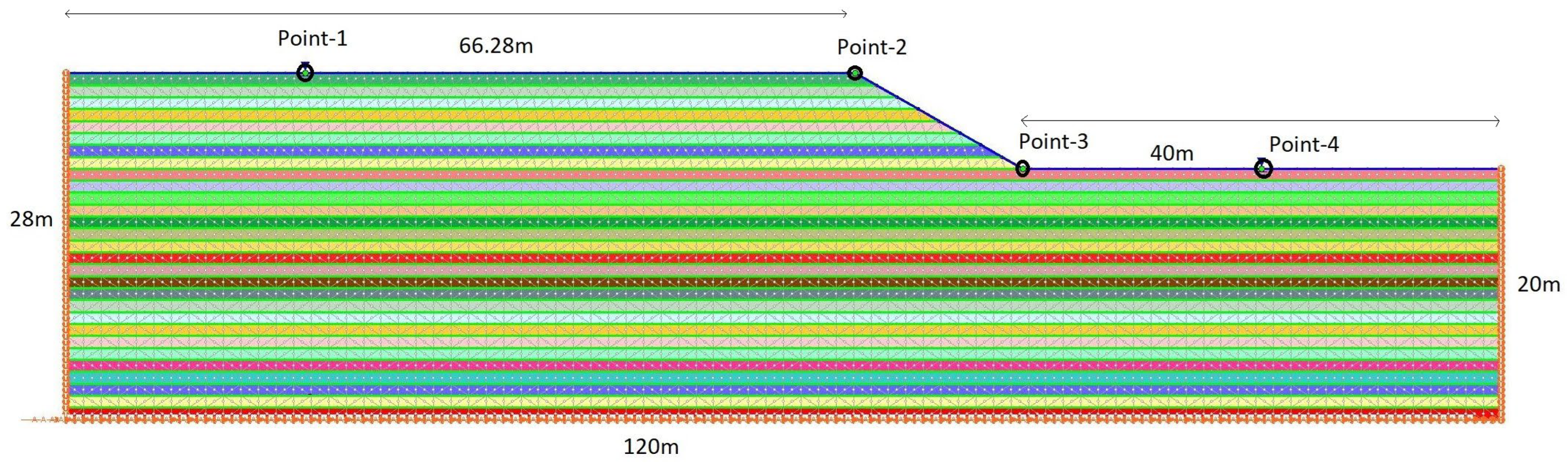
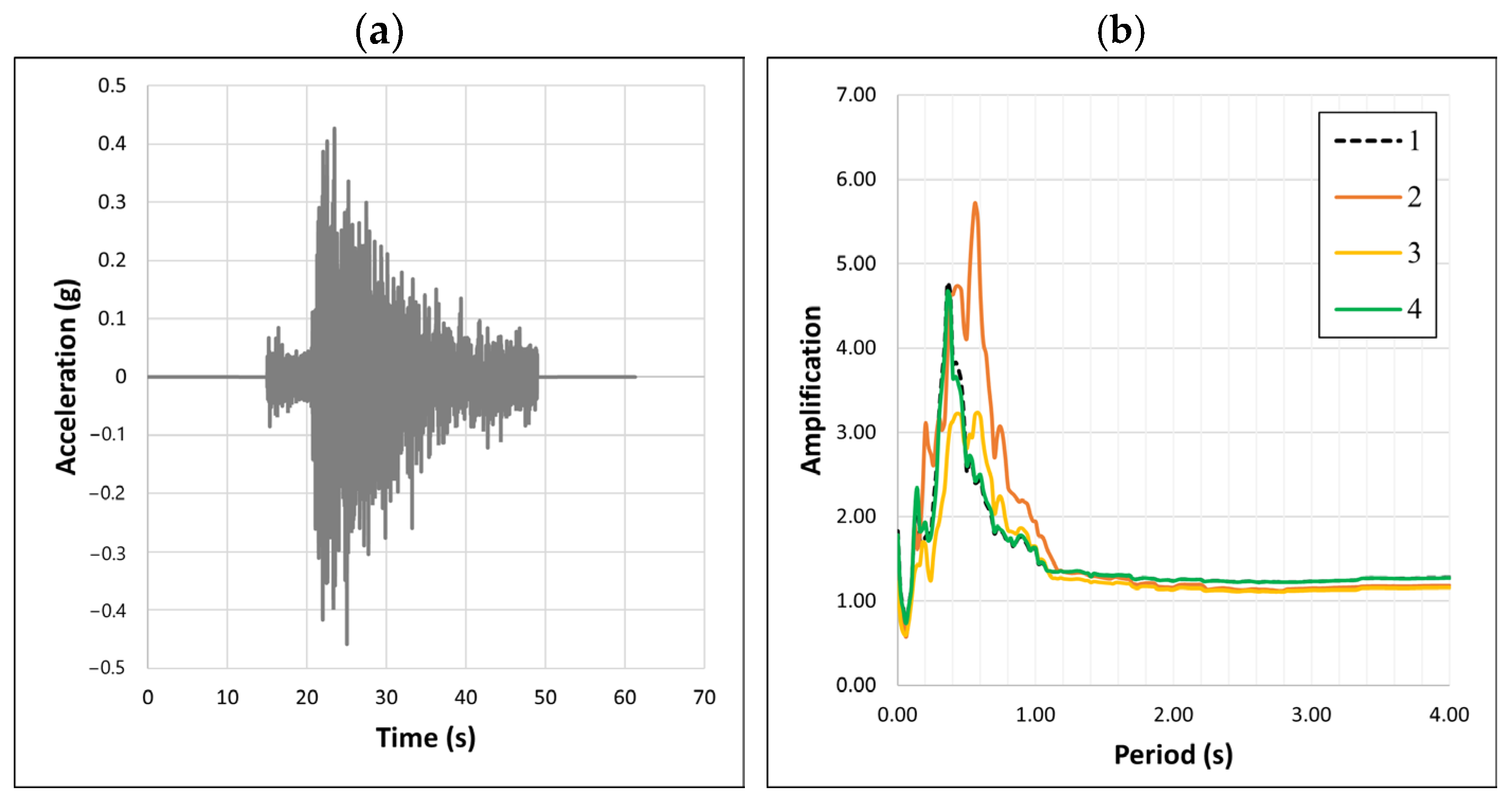
7.5. Illustrative Example: 2D FEM-Based Dynamic Analysis for Site Effect Estimation

A numerical analysis using the Finite Element Method (FEM) was utilized to evaluate the dynamic response of a slope, and the amplification was determined at different points. The slope geometry is shown in Figure 21. Shear-wave velocity and shear strength were derived from empirical correlations provided by [147,171], respectively, for eastern Canada. Material properties were defined for each 1 m thick layer (defined as different color in Figure 21); the last layer was considered rock. Different properties used in the dynamic FEM are shown in Appendix B (Table A3 and Table A4). The Saguenay 1988 earthquake motion, scaled to the NBCC 2020 design level with a 2% probability of exceedance in 50 years (2%/50 yrs PE), was used as input motion (Figure 22a). The RS2 software was applied to perform the dynamic analysis of the slope. Surface response accelerations were computed with the corresponding response spectra at the four points in Figure 21. The ratio of the surface response to the input earthquake motion was used to determine the site effect in terms of amplification.
The amplification functions, shown in Figure 22b, demonstrate significant variation in the seismic response across four slope points. Point #2, located at the crest, exhibits the highest amplification of around 5–6 times the input motion due to wave focusing, reduced confining pressure, and geometric effects; points #1 and #4, situated on relatively flat surfaces, show similar maximum amplification levels of about 4, as these areas experience uniform seismic energy distribution with less influence from slope geometry. In contrast, point #3, near the toe of the slope, has the lowest amplification, approximately 3 times, as seismic energy dissipates and compressive effects dominate in this zone. It can also be observed in Figure 22b that amplification is most pronounced for shorter periods (high-frequency waves) and decreases significantly beyond a period of 1 s, leveling off to match approximately the input motion at all points. Such behavior reflects the combined influence of slope geometry, material properties, and seismic wave interactions.
Figure 23 depicts a contour plot of maximum dynamic horizontal displacement (X-displacement). The highest displacement is concentrated on the slope, near the slope crest, as highlighted by the red and orange regions. The displacement gradually diminishes as the distance increases from the slope, transitioning through yellow, green, blue, and darker blue zones, indicating progressively lower displacement values. The maximum observed displacement is 4.12 × 10⁻² m at the slope of the model, while the minimum displacement, approximately 2.56 × 10⁻² m, is observed at the model’s base and edges.

8. Conclusions and Discussion

Predicting surface ground motion is important in quantifying the seismic hazards and understanding the potentially damaging effects during strong earthquake motion. It is well-established that local site conditions significantly influence the amplitude–frequency content, and duration of bedrock earthquake motions. The primary challenge in evaluating these impacts consists of determining representative site-specific soil properties and evaluating the intensity of the seismic shaking for reference site conditions, applying appropriate site effect proxies, and/or conducting numerical site response analyses. The latter is particularly relevant in cases without strong earthquake records, preferably simultaneous records on soft surficial soils and nearby rock outcrops. This is of common concern in regions of low to moderate seismicity. This paper addresses the major components of the site response analysis through a comprehensive review of an extensive list of references. The following are the key points of the review:
(i)
Site Effects
Site effects can significantly impact incoming seismic waves and vary depending on the local geological and geotechnical conditions. The most frequent site effects are the resonance amplification in a relatively uniform soft soil layer over bedrock with a sharp impedance contrast. This results in a single well-defined peak at the fundamental vibration period; multiple peak amplification corresponds to the presence of distinct heterogeneous surficial layers; and broadband amplification, which develops when soil stiffness increases with depth, generates a broad range of amplified frequencies rather than a single peak. On the other hand, topographic amplification is induced by focusing seismic waves in elevated features such as hills and ridges, leading to increased wave amplitudes. Basin-edge effects occur when seismic waves propagate in soft sediments with a gradually decreasing depth at the edges of sedimentary basins, resulting in an amplitude increase. Similarly, the basin effect involves trapping and reverberating seismic waves within a concave basin filled with soft sediments, amplifying ground motion and prolonging shaking duration. These potential effects require attention while evaluating the seismic hazard for structural design and risk assessment.
(ii)
Soil Parameters
Soil parameters important for evaluating the seismic site response include the shear-wave velocity, density, shear modulus reduction, and damping ratio curves. Collectively, these help determine how seismic waves are amplified or attenuated as they travel through the soil layers.
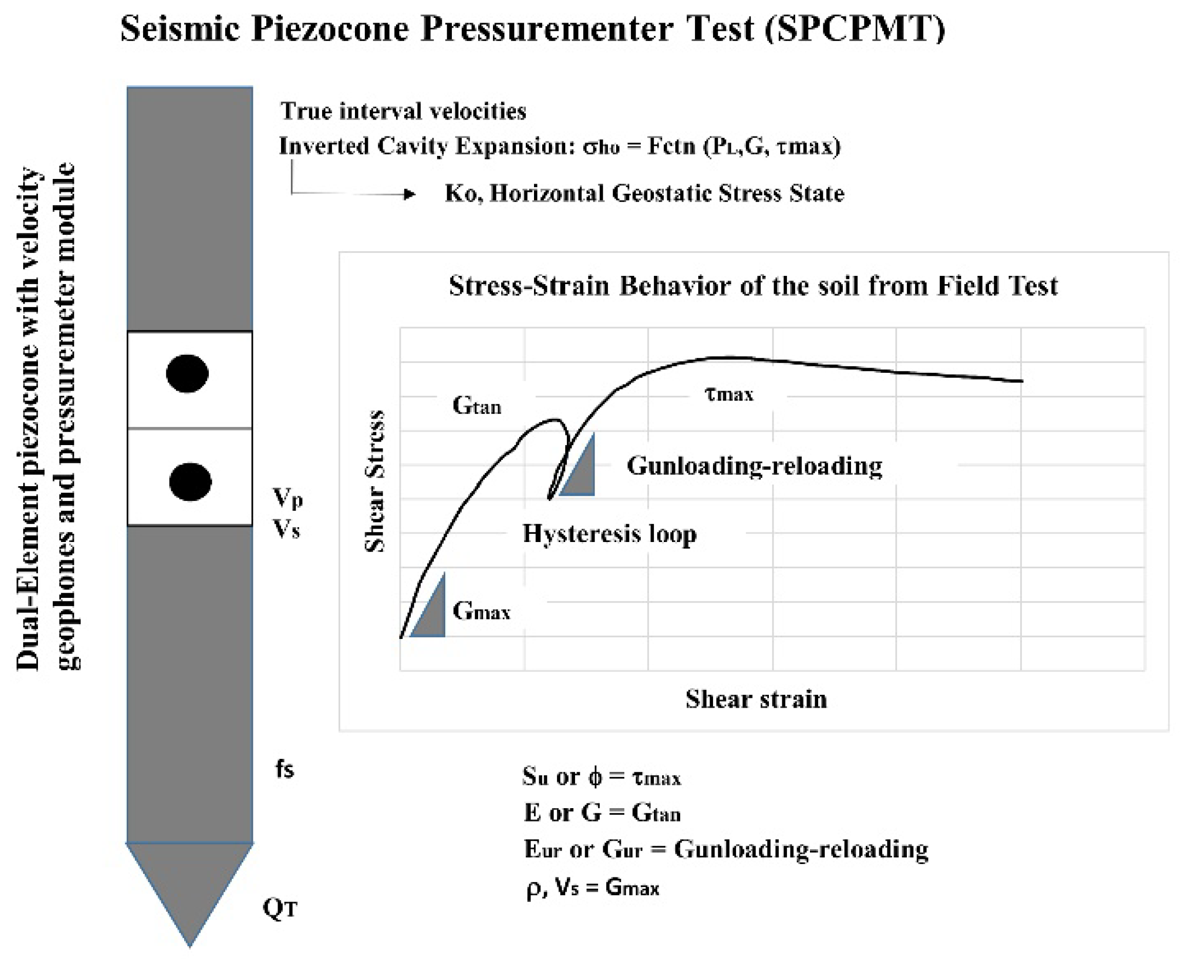
Among the existing field tests, the seismic cone penetration test (SCPT) or suspension logging yields highly accurate shear-wave velocity (VS) results. However, it is often costly and challenging to perform in gravelly soil. On the other hand, non-invasive geophysical methods are more applicable in various soil conditions and can provide a broader range of VS profiles. The setback is that they must be validated against results from at least one invasive investigation at similar/nearby sites to ensure accuracy. In addition, empirical correlations developed between different SCPT parameters can be combined with numerous CPT results when readily available for the study area.
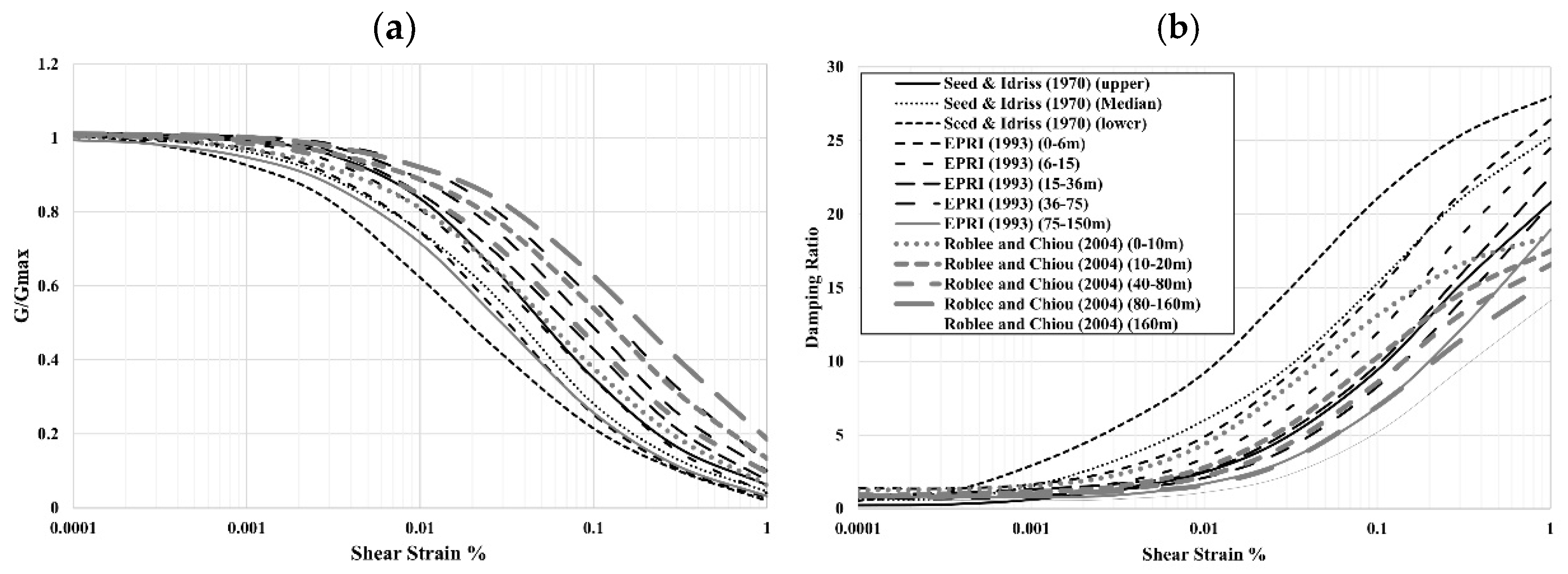
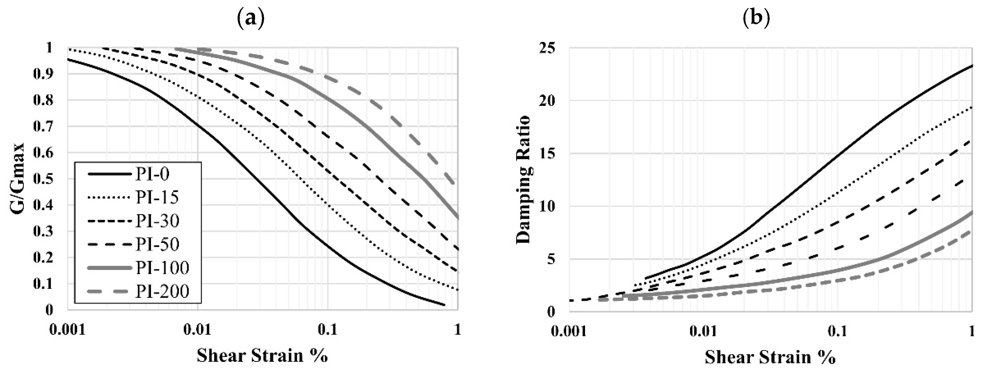
Shear modulus and damping ratio curves are critical for the characterization of the soil’s nonlinear behavior during earthquake shaking. They define how the soil stiffness (shear modulus) and energy dissipation (damping ratio) vary with strain levels. These parameters are essential for realistic seismic site response analyses as they directly influence ground motion amplification and deformation. Both curves are obtained through laboratory tests tailored to the specific application and soil type, such as resonant column, cyclic triaxial tests, or cyclic direct, simple shear tests. The factors influencing these parameters must be carefully considered for cohesive and cohesionless soils. For example, plasticity, water content, and over-consolidation ratio significantly impact cohesive soils’ modulus reduction and damping behavior. In contrast, more critical factors in cohesionless soils are the particle size distribution, relative density, and adequate confining pressure. Proper evaluation of these factors ensures reliable selection or development of shear modulus and damping ratio curves for dynamic analyses.
(iii)
Seismic parameters
The selection of representative ground motions accounts for seismic settings in the study area, the amplitude–frequency content, and the duration of the ground motions. To ensure consistency with the seismic hazard at the site, the selected ground motions can be matched to the target response spectrum at periods of interest. Herein, a detailed summary of reference rock conditions, seismic hazard assessment, and the selection and scaling of earthquake motions is provided.
The impacts of the complex medium, through which seismic waves propagate from the source fault, can be divided into two parts: the source-to-site propagation part, commonly determined with the ground motions from semi-empirical ground motion prediction equations, GMPEs, and the amplification part approximated with horizontal shear waves propagating vertically from the reference rock conditions. This interface is commonly defined as VS30 = 760∼800 m/s (B/C boundary) and measured with geophysical surveys or geotechnical investigations for engineering purposes.
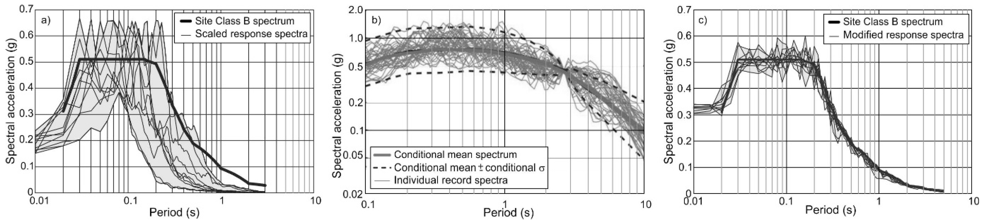
The seismic hazard at reference rock conditions is determined based on the seismic sources affecting the studied location, respective magnitude–frequency relationships, and applicable GMPEs. Probabilistic seismic hazard analysis yields the uniform hazard spectrum (UHS) with spectral accelerations (Sa) as the common ground motion output with the same exceedance probability. UHS is the maximum possible Sa value generated from different earthquake events in each period. Less conservative options are the conditional mean response spectrum (CMS) and conditional response spectrum (CS), which consider the intercorrelations between Sa at different periods.
To evaluate the potential amplification with numerical analyses, a suite of at least seven acceleration representative time histories is commonly recommended. When the number of strong earthquake records collected is insufficient, synthetic or ground motions from other regions with similar seismotectonic settings (magnitude, fault rupture mechanisms, source-to-site distance, and reference site conditions) may be used. Regarding the amplitude–frequency content, time histories are typically scaled to match the hazard spectrum at periods of interest in the time domain. Frequency-matching techniques can reproduce spectral accelerations across all periods; however, it would be highly unlikely to expect a single earthquake event to reach the maximum Sa values of the UHS. When there is a baseline drift, baseline correction is mandatory before the dynamic analyses.
(iv)
Site parameters
Site effects can be accounted for using simple amplification factors defined as the ratio of the response spectral accelerations at the ground surface to those at the bedrock level. The amplification factors are typically provided in national hazard maps. They are commonly applied in ground motion models (GMMs) to correlate the spectral accelerations at reference site conditions to earthquake parameters such as magnitude and distance. GMMs use various proxies to represent site conditions, including the average shear-wave velocity over the top 30 m (Vs30), soil fundamental period (T0), soil thickness (H), and others. However, relying solely on a single proxy, such as Vs30, may introduce bias and/or uncertainty, as it may not fully capture the complex nature of the site effects. Incorporating multiple proxies can improve the reliability and accuracy of GMMs by providing a more comprehensive representation of the site conditions.
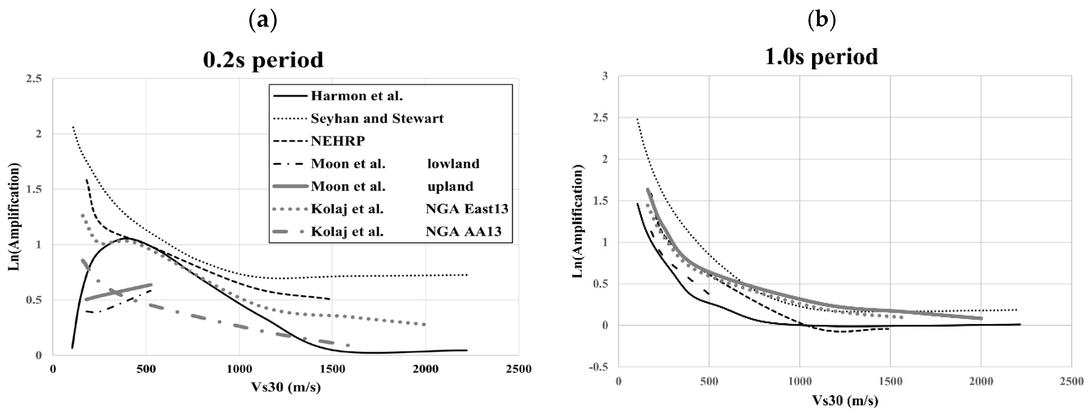
VS30 is undoubtedly the most frequently used proxy recommended in the building codes. A standard site classification scheme according to VS30 ranges includes site categories with similar amplification potential, such as hard rock, moderately fractured and weathered rock, stiff and dense soil, loose sandy soil, and soft clayey soil. For each site category, a respective amplification factor is provided. More recent building codes provide an amplification factor concerning VS30 as a continual function. However, the VS30 concept was developed based mainly on studies in California, where soft surficial soils gradually transform to regolith and rock without distinct impedance contrast. As such, it is not always correlated with the amplification observed in regions with high impedance contrast at the bedrock interface.
On the other hand, T0 reflects the vibration period at which the seismic waves are expected to be most amplified. It is measured relatively easily using horizontal-to-vertical spectral ratio (HVSR) field measurements, which provide direct and practical insights into the resonance characteristics of the site. However, since the ambient noise does not induce significant strain, HVSR cannot account for the nonlinear behavior of soil during strong ground motion, thus overestimating the actual amplification. Alternatively, T0 can be calculated analytically if the soil thickness and in-depth shear-wave velocity are known. While the commonly used quarter wavelength equation (T = 4H/Vs) is simple and widely applied, it appears limited to relatively shallow soil layers. To improve accuracy, other analytical approaches that account for complex soil stratification, varying velocity profiles, and impedance contrasts should be considered, offering more precise estimations of the fundamental site period depending on site-specific conditions.
(v)
Experimental and Numerical evaluation
Several methods for the prediction of the site response were considered. The standard spectral ratio method is based on at least two ground motions recorded on the soil surface and nearby rock outcrop. It compares the response spectral accelerations of both records and provides a more realistic estimation of the potential site amplification in that area. The soil dynamic response can also be simulated numerically in 1D, 2D, or 3D, adopting linear, equivalent linear, or nonlinear approaches. In 1D analysis, the horizontal seismic shear waves are assumed to propagate vertically through the infinite horizontal soil layers, making it suitable for sites with simple stratigraphy. 2D and 3D site response analyses are preferred for more complex soil conditions or irregular geometries as they account for lateral variations and interactions. The linear analysis assumes that soil behavior can be modeled as a linear elastic material with a constant minimum damping ratio and maximum shear modulus assigned to each soil unit. In this way, it simplifies the analysis at the expense of soil nonlinearity. The equivalent linear analysis approximates nonlinearity iteratively by assigning updated linear properties to each layer at the beginning of each step based on the attained shear modulus and damping ratio curves and the adequate strain levels. In contrast, nonlinear analysis directly integrates the equation of motion in the time domain, applying stress–strain relationships to calculate soil properties dynamically at each time step. Nonlinear analysis is most accurate as it fully considers the total nonlinearity of soil under earthquake loading and is particularly suitable for high-strain conditions. However, the challenge is obtaining appropriate nonlinear curves for the soil units in the study area that reliably capture the actual response during intense earthquake shaking.

Author Contributions

Conceptualization, M.S. and A.S.; methodology, A.S.M.F.H.; software, A.S.M.F.H.; validation, M.N., M.S. and A.S.; formal analysis, A.S.M.F.H.; investigation, A.S.M.F.H.; resources, M.S., A.S. and J.R.S.; data curation, A.S.M.F.H.; writing—original draft preparation, A.S.M.F.H.; writing—review and editing, M.N., M.S., A.S., J.R.S. and Z.B.; visualization, A.S.M.F.H.; supervision, A.S. and M.N.; project administration, A.S.; funding acquisition, A.S. All authors have read and agreed to the published version of the manuscript.

Funding

The authors declare the following financial interests/personal relationships which may be considered as potential competing interests: Ali Saeidi reports financial support was provided by Natural Sciences and Engineering Research Council of Canada, Hydro-Quebec (CRDPJ 521771-17). Ali Saeidi reports financial support was provided by Natural Sciences and Engineering Research Council of Canada, Hydro-Quebec, Geostack, Rocscience and City of Saguenay (ALLRP 590081-23). If there are other authors, they declare that they have no known competing financial interests or personal relationships that could have appeared to influence the work reported in this paper.

Conflicts of Interest

Juliana Ruiz Suescun was employed by the company Hydro Québec. The remaining authors declare that the research was conducted in the absence of any commercial or financial relationships that could be construed as a potential conflict of interest.

Appendix A

Table A1. Different Methods.
MethodLayerName of MethodReferences
BasicSingleConstant distribution of shear-wave velocity with depth[142]
Method-1Singleπ times the travel time of the shear-wave velocity method[144]
Method-2SinglePower-law distribution of the shear-wave method[82]
Method-3SingleLinear distribution of shear modulus with depth method[141,142]
Method-4DoubleConstant distribution of shear-wave velocity with depth[142]
Method-5DoubleSimplified Rayleigh’s method[145]
Method-6DoubleLinear fundamental mode shape[145]
Table A2. Soil Fundamental period and deviation of different methods with the basic method.
H (m)Vsavg (m/s)Basic (s)M1 (s)M2 (s)M3 (s)M4 (s)M5 (s)M6 (s)Deviation M1Deviation M2Deviation M3Deviation M4Deviation M5Deviation M6
M1101500.270.210.230.230.340.170.26−21.46−13.90−13.8129.15−37.65−1.23
M2201600.500.390.410.410.610.300.47−21.46−18.30−18.2222.54−40.84−6.28
M3301800.670.520.500.500.750.360.58−21.46−24.73−24.6512.91−45.49−13.65
M4401900.840.660.610.610.920.440.70−21.46−27.14−27.069.30−47.24−16.42
M5602001.200.940.850.851.270.620.97−21.46−29.18−29.116.23−48.72−18.76
M6802101.521.201.051.051.580.761.21−21.46−30.93−30.863.61−49.99−20.77
M71002201.821.431.231.231.840.891.41−21.46−32.45−32.381.33−51.09−22.51
M81502502.401.881.541.542.301.111.76−21.46−35.99−35.93−3.99−53.65−26.58
M92002902.762.171.681.682.511.211.92−21.46−39.22−39.16−8.83−55.99−30.28
M102503203.132.451.841.852.771.342.12−21.46−40.97−40.91−11.45−57.25−32.28
M113003503.432.691.981.982.971.432.27−21.46−42.34−42.28−13.50−58.25−33.85
M123503803.682.892.082.093.131.512.39−21.46−43.44−43.39−15.16−59.05−35.12
M134004103.903.062.172.173.261.572.49−21.46−44.35−44.30−16.53−59.71−36.17
M144504204.293.372.372.383.561.722.72−21.46−44.62−44.57−16.93−59.90−36.47
M155004304.653.652.562.573.851.862.94−21.46−44.88−44.82−17.32−60.09−36.77
M166004405.454.282.993.004.492.173.43−21.46−45.12−45.06−17.68−60.26−37.04
M177004506.224.893.403.405.102.463.90−21.46−45.35−45.29−18.02−60.42−37.30
M188004606.965.463.793.795.682.744.34−21.46−45.56−45.51−18.34−60.58−37.55
M199004707.666.024.154.166.233.014.77−21.46−45.77−45.71−18.65−60.73−37.79
M2010004758.426.614.564.566.843.305.23−21.46−45.87−45.81−18.80−60.80−37.90
M2111004809.177.204.954.967.433.595.68−21.46−45.96−45.91−18.94−60.87−38.01
M2212004859.907.775.345.348.013.876.12−21.46−46.06−46.00−19.08−60.94−38.12
M23130049010.618.335.715.728.574.146.56−21.46−46.15−46.09−19.22−61.01−38.22
M24140049511.318.896.086.099.124.406.98−21.46−46.24−46.18−19.36−61.07−38.33
M25150050012.009.426.446.459.664.667.39−21.46−46.33−46.27−19.49−61.13−38.43

Appendix B

Table A3. Unit weight of different materials used in dynamic FEM.
TypeUnit Weight
Clay18.17kN/m3
Rock28kN/m3
Table A4. Strength and stiffness properties of soil and rock used in dynamic FEM.
DepthVS (m/s)Gmax (Mpa)E (Mpa)Su (kPa)
1124287758
2130328564
3136349370
41413710076
51464010781
61514211487
71564512192
81604812898
916450135103
1016953142109
1117355149114
1217758156119
1318160163125
1418463170130
1518866177136
1619268184141
1719571191147
1819973198153
1920376205158
2020679212164
2121081220170
2221384227175
2321687234181
2422089241187
2522392249193
2622695256199
2723098264205
28233100271211
Rock1875651217,58215,266

References

  1. Kramer, S.L. Geotechnical Earthquake Engineering; Pearson Education: Hoboken, NJ, USA, 1996. [Google Scholar]
  2. Hunter, J.A.M.; Crow, H.L. Shear Wave Velocity Measurement Guidelines for Canadian Seismic Site Characterization in Soil and Rock; Natural Resources Canada: Gatineau, QC, Canada, 2015. [Google Scholar]
  3. Naggar, E. Geotechnical Earthquake Engineering; CRC Press: Toronto, ON, Canada, 2010. [Google Scholar]
  4. Nastev, M.; Parent, M.; Ross, M.; Howlett, D.; Benoit, N. Geospatial modelling of shear-wave velocity and fundamental site period of Quaternary marine and glacial sediments in the Ottawa and St. Lawrence Valleys, Canada. Soil Dyn. Earthq. Eng. 2016, 85, 103–116. [Google Scholar] [CrossRef]
  5. Kwon, O.-S.; Elnashai, A.S. Distributed analysis of interacting soil and structural systems under dynamic loading. Innov. Infrastruct. Solut. 2017, 2, 30. [Google Scholar] [CrossRef]
  6. Dobry, R. Dynamic properties and seismic response of soft clay deposits. Proc. Int. Symp. Geotech. Engrg. Soft Soils 1987, 2, 51–87. [Google Scholar]
  7. Clayton, C. Stiffness at small strain: Research and practice. Géotechnique 2011, 61, 5–37. [Google Scholar] [CrossRef]
  8. Luna, R.; Jadi, H. Determination of dynamic soil properties using geophysical methods. In Proceedings of the First International Conference on the Application of Geophysical and NDT Methodologies to Transportation Facilities and Infrastructure, St. Louis, MO, USA, 11–15 December 2000; pp. 1–15. [Google Scholar]
  9. John, A.; Stephen, H.; Trevor, A.; Garry, R. Canada’s 6th Generation Seismic Hazard Model, as Prepared for the 2020 National Building Code of Canada. In Proceedings of the 12th Canadian Conference on Earthquake Engineering, Quebec City, QC, Canada, 17–20 June 2015. [Google Scholar]
  10. Tremblay, R.; Atkinson, G.M.; Bouaanani, N.; Daneshvar, P.; Léger, P.; Koboevic, S. Selection and scaling of ground motion time histories for seismic analysis using NBCC 2015. In Proceedings of the 11th Canadian Conference on Earthquake Engineering (11CCEE), Victoria, BC, Canada, 21–24 July 2015; p. 69. [Google Scholar]
  11. Motazedian, D. Stochastic Finite-Fault Modeling Based on a Dynamic Corner Frequency. Bull. Seism. Soc. Am. 2005, 95, 995–1010. [Google Scholar] [CrossRef]
  12. Seed, H.B.; Idriss, I.M. Ground Motions and Soil Liquefaction During Earthquakes; Earthquake Engineering Research Insititue: Berkeley, CA, USA, 1982. [Google Scholar]
  13. Foulon, T.; Saeidi, A.; Chesnaux, R.; Nastev, M.; Rouleau, A. Spatial distribution of soil shear-wave velocity and the fundamental period of vibration—A case study of the Saguenay region, Canada. Georisk Assess. Manag. Risk Eng. Syst. Geohazards 2018, 12, 74–86. [Google Scholar] [CrossRef]
  14. Stone, W.C.; Yokel, F.Y.; Celebi, M. Engineering Aspects of the September 19, 1985 Mexico; Earthquake Engineering Research: Hyogo, Japan, 1987. [Google Scholar]
  15. Mayoral, J.; Asimaki, D.; Tepalcapa, S.; Wood, C.; la Sancha, A.R.-D.; Hutchinson, T.; Franke, K.; Montalva, G. Site effects in Mexico City basin: Past and present. Soil Dyn. Earthq. Eng. 2019, 121, 369–382. [Google Scholar] [CrossRef]
  16. Hossain, A.S.M.F.; Adhikari, T.L.; Ansary, M.A.; Bari, Q.H. Characteristics and Consequence of Nepal Earthquake 2015: A Review. Geotech. Eng. J. SEAGS AGSSEA 2015, 46, 114–120. [Google Scholar]
  17. Molnar, S.; Cassidy, J.F. A Comparison of Site Response Techniques Using Weak-Motion Earthquakes and Microtremors. Earthq. Spectra 2006, 22, 169–188. [Google Scholar] [CrossRef]
  18. Bouchon, M.; Barker, J.S. Seismic response of a hill: The example of Tarzana, California. Bull. Seism. Soc. Am. 1996, 86, 66–72. [Google Scholar] [CrossRef]
  19. Spudich, P.; Hellweg, M.; Lee, W.H.K. Directional topographic site response at Tarzana observed in aftershocks of the 1994 Northridge, California, earthquake: Implications for mainshock motions. Bull. Seism. Soc. Am. 1996, 86, S193–S208. [Google Scholar] [CrossRef]
  20. Abrahamson, N.A.; Somerville, P.G. Effects of the hanging wall and footwall on ground motions recorded during the Northridge earthquake. Bull. Seism. Soc. Am. 1996, 86, S93–S99. [Google Scholar] [CrossRef]
  21. Molnar, S.; Sirohey, A.; Assaf, J.; Bard, P.-Y.; Castellaro, S.; Cornou, C.; Cox, B.; Guillier, B.; Hassani, B.; Kawase, H.; et al. A review of the microtremor horizontal-to-vertical spectral ratio (MHVSR) method. J. Seism. 2022, 26, 653–685. [Google Scholar] [CrossRef]
  22. Graves, R.W.; Pitarka, A.; Somerville, P.G. Ground-motion amplification in the Santa Monica area: Effects of shallow basin-edge structure. Bull. Seism. Soc. Am. 1998, 88, 1224–1242. [Google Scholar] [CrossRef]
  23. Hossain, A.F.; Salsabili, M.; Saeidi, A.; Suescun, J.R.; Nastev, M. Effects of Shear Wave Velocity and Thickness of Soil Layers on 1D Dynamic Response in the Saguenay Region, Quebec. In Rocscience International Conference (RIC 2023); Atlantis Press: Toronto, ON, Canada, 2023; pp. 165–173. [Google Scholar] [CrossRef]
  24. Hossain, A.F.; Saeidi, A.; Salsabili, M.; Nastev, M.; Suescun, J.R. Soil Dynamic Response and Site Amplification Parameters for Saguenay, Eastern Canada. Jpn. Geotech. Soc. Spéc. Publ. 2024, 10, 1952–1957. [Google Scholar] [CrossRef]
  25. Hossain, A.F.; Saeidi, A.; Salsabili, M.; Nastev, M.; Suescun, J.R. Analytical and numerical investigation of the site response period in the Saguenay region, Eastern Canada. In Proceedings of the 3rd Croatian Conference on Earthquake Engineering (3CroCEE), Split, Croatia, 19–22 March 2025. [Google Scholar]
  26. Seed, H.B.; Romo, M.P.; Sun, J.I.; Jaime, A.; Lysmer, J. The Mexico Earthquake of September 19, 1985—Relationships Between Soil Conditions and Earthquake Ground Motions. Earthq. Spectra 1988, 4, 687–729. [Google Scholar] [CrossRef]
  27. Jackson, F.; Molnar, S.; Ghofrani, H.; Atkinson, G.M.; Cassidy, J.F.; Assatourians, K. Ground Motions of the December 2015 M 4.7 Vancouver Island Earthquake: Attenuation and Site Response. Bull. Seism. Soc. Am. 2017, 107, 2903–2916. [Google Scholar] [CrossRef]
  28. Klin, P.; Laurenzano, G.; Barnaba, C.; Priolo, E.; Parolai, S. Site Amplification at Permanent Stations in Northeastern Italy. Bull. Seism. Soc. Am. 2021, 111, 1885–1904. [Google Scholar] [CrossRef]
  29. Pratt, T.L. Amplification of Seismic Waves by the Seattle Basin, Washington State. Bull. Seism. Soc. Am. 2003, 93, 533–545. [Google Scholar] [CrossRef]
  30. Assimaki, D. Effects of Local Soil Conditions on the Topographic Aggravation of Seismic Motion: Parametric Investigation and Recorded Field Evidence from the 1999 Athens Earthquake. Bull. Seism. Soc. Am. 2005, 95, 1059–1089. [Google Scholar] [CrossRef]
  31. Meunier, P.; Hovius, N.; Haines, J.A. Topographic site effects and the location of earthquake induced landslides. Earth Planet. Sci. Lett. 2008, 275, 221–232. [Google Scholar] [CrossRef]
  32. Bard, P.-Y.; Bouchon, M. The two-dimensional resonance of sediment-filled valleys. Bull. Seism. Soc. Am. 1985, 75, 519–541. [Google Scholar] [CrossRef]
  33. Shabani, M.J.; Zakerinejad, M. Slope topographic impacts on the nonlinear seismic analysis of soil-foundation-structure interaction for similar MRF buildings. Soil Dyn. Earthq. Eng. 2022, 160, 107365. [Google Scholar] [CrossRef]
  34. Sitar, N.; Clough, G.W. Seismic Response of Steep Slopes in Cemented Soils. J. Geotech. Eng. 1983, 109, 210–227. [Google Scholar] [CrossRef]
  35. Bararpour, M.; Janalizade, A.; Tavakoli, H.R. The effect of 2D slope and valley on seismic site response. Arab. J. Geosci. 2016, 9, 93. [Google Scholar] [CrossRef]
  36. Zhang, Z.; Fleurisson, J.-A.; Pellet, F. The effects of slope topography on acceleration amplification and interaction between slope topography and seismic input motion. Soil Dyn. Earthq. Eng. 2018, 113, 420–431. [Google Scholar] [CrossRef]
  37. Bard, P.-Y.; Riepl-Thomas, J. Wave Propagation in Complex Geological Structures and Their Effects on Strong Ground Motion. 2000. Available online: https://www.researchgate.net/publication/235623287 (accessed on 17 March 2025).
  38. Molnar, S.; Cassidy, J.F.; Olsen, K.B.; Dosso, S.E.; He, J. Earthquake Ground Motion and 3D Georgia Basin Amplification in Southwest British Columbia: Deep Juan de Fuca Plate Scenario Earthquakes. Bull. Seism. Soc. Am. 2014, 104, 301–320. [Google Scholar] [CrossRef]
  39. Molnar, S.; Cassidy, J.F.; Olsen, K.B.; Dosso, S.E.; He, J. Earthquake Ground Motion and 3D Georgia Basin Amplification in Southwest British Columbia: Shallow Blind-Thrust Scenario Earthquakes. Bull. Seism. Soc. Am. 2014, 104, 321–335. [Google Scholar] [CrossRef]
  40. Marafi, N.A.; Eberhard, M.O.; Berman, J.W.; Wirth, E.A.; Frankel, A.D. Impacts of Simulated M9 Cascadia Subduction Zone Motions on Idealized Systems. Earthq. Spectra 2019, 35, 1261–1287. [Google Scholar] [CrossRef]
  41. Kakoty, P.; Dyaga, S.M.; Hutt, C.M. Impacts of simulated M9 Cascadia Subduction Zone earthquakes considering amplifications due to the Georgia sedimentary basin on reinforced concrete shear wall buildings. Earthq. Eng. Struct. Dyn. 2021, 50, 237–256. [Google Scholar] [CrossRef]
  42. Rekoske, J.M.; Moschetti, M.P.; Thompson, E.M. Basin and Site Effects in the U.S. Pacific Northwest Estimated from Small-Magnitude Earthquakes. Bull. Seism. Soc. Am. 2022, 112, 438–456. [Google Scholar] [CrossRef]
  43. Petersen, M.D.; Shumway, A.M.; Powers, P.M.; Mueller, C.S.; Moschetti, M.P.; Frankel, A.D.; Rezaeian, S.; McNamara, D.E.; Luco, N.; Boyd, O.S.; et al. The 2018 update of the US National Seismic Hazard Model: Overview of model and implications. Earthq. Spectra 2020, 36, 5–41. [Google Scholar] [CrossRef]
  44. Kakoty, P.; Hutt, C.M.; Ghofrani, H.; Molnar, S. Spectral acceleration basin amplification factors for interface Cascadia Subduction Zone earthquakes in Canada’s 2020 national seismic hazard model. Earthq. Spectra 2023, 39, 1166–1188. [Google Scholar] [CrossRef]
  45. Hossain, A.S.M.F.; Ansary, M.A. PS Logging for Site Response Analysis in Dhaka City. Aust. J. Sci. Technol. 2017, 6, 83–99. [Google Scholar]
  46. Kamalb, D.E.H.A.M.; Alama, A.W.U.M.B. Comparison of Shear Wave Velocity Derived from PS Logging and MASW—A Case Study of Mymensingh Pourashava, Bangladesh. Bangladesh J. Geol. 2013, 26, 84–97. [Google Scholar]
  47. Salsabili, M.; Saeidi, A.; Rouleau, A.; Nastev, M. Development of empirical CPTu-V correlations for post-glacial sediments in Southern Quebec, Canada, in consideration of soil type and geological setting. Soil Dyn. Earthq. Eng. 2022, 154, 107131. [Google Scholar] [CrossRef]
  48. Nastev, M.; Parent, M.; Benoit, N.; Ross, M.; Howlett, D. Regional VS30model for the St. Lawrence Lowlands, Eastern Canada. Georisk Assess. Manag. Risk Eng. Syst. Geohazards 2016, 10, 200–212. [Google Scholar] [CrossRef]
  49. Mayne, P.W.; Rix, G.J. Correlations Between Shear Wave Velocity and Cone Tip Resistance in Natural Clays. Soils Found. 1995, 35, 107–110. [Google Scholar] [CrossRef]
  50. Madiai, C.; Simoni, G. Shear wave velocity-penetration resistance correlation for Holocene and Pleistocene soils of an area in central Italy. In ISC-2 on Geotechnical and Geophysical Site Characterization; da Fonseca, V., Mayne, Eds.; Millpress: Rotterdam, The Netherlands, 2004; ISBN 9059660099. [Google Scholar]
  51. Hegazy, Y.A.; Mayne, P.W. A Global Statistical Correlation between Shear Wave Velocity and Cone Penetration Data. In Proceedings of the Geo Shanghai International Conference 2006, Shanghai, China, 6–8 June 2006; pp. 243–248. [Google Scholar] [CrossRef]
  52. Andrus, R.D.; Mohanan, N.P.; Piratheepan, P.; Ellis, B.S.; Holzer, T.L. Predicting Shear-Wave Velocity from Cone Penetration Resistance. In Proceedings of the 4th International Conference on Earthquake Geotechnical Engineering, Thessaloniki, Greece, 25–28 June 2007. [Google Scholar]
  53. Long, M.; Donohue, S. Characterization of Norwegian marine clays with combined shear wave velocity and piezocone cone penetration test (CPTU) data. Can. Geotech. J. 2010, 47, 709–718. [Google Scholar] [CrossRef]
  54. Tonni, L.; Simonini, P. Shear wave velocity as function of cone penetration test measurements in sand and silt mixtures. Eng. Geol. 2013, 163, 55–67. [Google Scholar] [CrossRef]
  55. McGann, C.R.; Bradley, B.A.; Taylor, M.L.; Wotherspoon, L.M.; Cubrinovski, M. Development of an empirical correlation for predicting shear wave velocity of Christchurch soils from cone penetration test data. Soil Dyn. Earthq. Eng. 2015, 75, 66–75. [Google Scholar] [CrossRef]
  56. Perret, D.; Charrois, E.; Bolduc, M. Shear Wave Velocity Estimation from Piezocone Test Data for Eastern Canada Sands (Quebec and Ontario)—Extended Version with Appendices; Natural Resources Canada: Gatineau, QC, Canada, 2016. [Google Scholar] [CrossRef]
  57. L’Heureux, J.-S.; Long, M. Relationship between Shear-Wave Velocity and Geotechnical Parameters for Norwegian Clays. J. Geotech. Geoenvironmental Eng. 2017, 143, 04017013. [Google Scholar] [CrossRef]
  58. Karray, M.; Hussien, M.N. Shear wave velocity as function of cone penetration resistance and grain size for Holocene-age uncemented soils: A new perspective. Acta Geotech. 2017, 12, 1129–1158. [Google Scholar] [CrossRef]
  59. Tong, L.; Che, H.; Zhang, M.; Pan, H. Determination of shear wave velocity of Yangtze Delta sediments using seismic piezocone tests. Transp. Geotech. 2018, 14, 29–40. [Google Scholar] [CrossRef]
  60. Pelekis, P.; Athanasopoulos, G. An overview of surface wave methods and a reliability study of a simplified inversion technique. Soil Dyn. Earthq. Eng. 2011, 31, 1654–1668. [Google Scholar] [CrossRef]
  61. Aki, K. Space and Time Spectra of Stationary Stochastic Waves, with Special Reference to Microtremors; Bulletin Earth Research Institute: Tsukuba City, Japan, 1957; pp. 415–456. [Google Scholar]
  62. Kocaoğlu, A.H.; Fırtana, K. Estimation of shear wave velocity profiles by the inversion of spatial autocorrelation coefficients. J. Seism. 2011, 15, 613–624. [Google Scholar] [CrossRef]
  63. Asten, M.W.; Hayashi, K. Application of the Spatial Auto-Correlation Method for Shear-Wave Velocity Studies Using Ambient Noise. Surv. Geophys. 2018, 39, 633–659. [Google Scholar] [CrossRef]
  64. Pan, Q.; Shen, X.; Ye, X.; Wang, L. Fine Shear-Wave Velocity Structures of Subsurface beneath the Guangdong–Hong Kong–Macao Greater Bay Area with Dense Seismic Array and SPAC Method. Seism. Res. Lett. 2024, 95, 2894–2909. [Google Scholar] [CrossRef]
  65. Ling, S.; Okada, H. An extended use of the spatial autocorre lation method for the estimation of structure using microtremors. In Proceedings of the 89th SEGJ Conference, Nagoya, Japan, 12–14 October 1993; Society of Exploration Geophysicists of Japan: Nagoya, Japan, 1993. [Google Scholar]
  66. Ohori, M. A Comparison of ESAC and FK Methods of Estimating Phase Velocity Using Arbitrarily Shaped Microtremor Arrays. Bull. Seism. Soc. Am. 2002, 92, 2323–2332. [Google Scholar] [CrossRef]
  67. Moro, G.D. Effective Active and Passive Seismics for the Characterization of Urban and Remote Areas: Four Channels for Seven Objective Functions. Pure Appl. Geophys. 2019, 176, 1445–1465. [Google Scholar] [CrossRef]
  68. Mantovani, A.; Abu Zeid, N.; Bignardi, S.; Tarabusi, G.; Santarato, G.; Caputo, R. Seismic Noise-Based Strategies for Emphasizing Recent Tectonic Activity and Local Site Effects: The Ferrara Arc, Northern Italy, Case Study. Pure Appl. Geophys. 2019, 176, 2321–2347. [Google Scholar] [CrossRef]
  69. Aki, K. A Note on The Use of Microseisms in Determining the Shallow Structures of the Earth’s Crust. Geophysics 1965, 30, 665–666. [Google Scholar] [CrossRef]
  70. Capon, J. High-resolution frequency-wavenumber spectrum analysis. Proc. IEEE 1969, 57, 1408–1418. [Google Scholar] [CrossRef]
  71. Lacoss, R.T.; Kelly, E.J.; Toksöz, M.N. S-wave velocity structure and site effect parameters derived from microtremor arrays in the Western Plain of Taiwan. Geophysics 1969, 34, 21–38. [Google Scholar] [CrossRef]
  72. Kuo, C.-H.; Chen, C.-T.; Lin, C.-M.; Wen, K.-L.; Huang, J.-Y.; Chang, S.-C. S-wave velocity structure and site effect parameters derived from microtremor arrays in the Western Plain of Taiwan. J. Asian Earth Sci. 2016, 128, 27–41. [Google Scholar] [CrossRef]
  73. Cheng, F.; Xia, J.; Xu, Z.; Hu, Y.; Mi, B. Frequency–Wavenumber (FK)-Based Data Selection in High-Frequency Passive Surface Wave Survey. Surv. Geophys. 2018, 39, 661–682. [Google Scholar] [CrossRef]
  74. Louie, J.N. Faster, Better: Shear-Wave Velocity to 100 Meters Depth from Refraction Microtremor Arrays. Bull. Seism. Soc. Am. 2001, 91, 347–364. [Google Scholar] [CrossRef]
  75. Song, Y.Y.; Castagna, J.P.; Black, R.A.; Knapp, R.W. Sensitivity of Near-Surface Shear-Wave Velocity Deter Mination from Rayleigh and Love Waves; Society of Exploration Geophysicists: Houston, TX, USA, 1989. [Google Scholar]
  76. Xia, J.; Miller, R.D.; Park, C.B. Estimation of near-surface shear-wave velocity by inversion of Rayleigh waves. Geophysics 1999, 64, 691–700. [Google Scholar] [CrossRef]
  77. Cheng, F.; Xia, J.; Luo, Y.; Xu, Z.; Wang, L.; Shen, C.; Liu, R.; Pan, Y.; Mi, B.; Hu, Y. Multichannel analysis of passive surface waves based on crosscorrelations. Geophysics 2016, 81, EN57–EN66. [Google Scholar] [CrossRef]
  78. Fernandes, J.B.; Rocha, B.P.; Giacheti, H.L. Maximum shear modulus and modulus degradation curves of an unsaturated tropical soil. Soils Rocks 2023, 46, e2023013122. [Google Scholar] [CrossRef]
  79. Zayed, M.; Ebeido, A.; Prabhakaran, A.; Kim, K.; Qiu, Z.; Elgamal, A. Shake Table Testing: A High-Resolution Vertical Accelerometer Array for Tracking Shear Wave Velocity. Geotech. Test. J. 2021, 44, 1097–1118. [Google Scholar] [CrossRef]
  80. Lee, C.-J.; Wang, C.-R.; Wei, Y.-C.; Hung, W.-Y. Evolution of the shear wave velocity during shaking modeled in centrifuge shaking table tests. Bull. Earthq. Eng. 2012, 10, 401–420. [Google Scholar] [CrossRef]
  81. Likitlersuang, S.; Teachavorasinskun, S.; Surarak, C.; Oh, E.; Balasubramaniam, A. Small strain stiffness and stiffness degradation curve of Bangkok Clays. Soils Found. 2013, 53, 498–509. [Google Scholar] [CrossRef]
  82. Idriss, I.M.; Seed, H.B. Seismic Response of Horizontal Soil Layers. J. Soil Mech. Found. Div. 1968, 94, 1003–1031. [Google Scholar] [CrossRef]
  83. Mohammadioun, B. Nonlinear Response of Soils to Horizontal and Vertical Bedrock Earthquake Motion. J. Earthq. Eng. 1997, 1, 93–119. [Google Scholar] [CrossRef]
  84. Mayne, P.W. Stress-strain-strength-flow parameters from enhanced in-situ tests. In Proceedings of the In-Situ Measurement of Soil Properties & Case Histories, Bali, Indonesia, 21–24 May 2001; pp. 27–47. [Google Scholar]
  85. Fahey, M.; Carter, J.P. A finite element study of the pressuremeter test in sand using a nonlinear elastic plastic model. Can. Geotech. J. 1993, 30, 348–362. [Google Scholar] [CrossRef]
  86. Baghbani, A.; Choudhury, T.; Samui, P.; Costa, S. Prediction of secant shear modulus and damping ratio for an extremely dilative silica sand based on machine learning techniques. Soil Dyn. Earthq. Eng. 2023, 165, 107708. [Google Scholar] [CrossRef]
  87. Saathoff, J.-E.; Achmus, M. Excess pore pressure accumulation in sands—A shear strain threshold concept for optimization of a laboratory testing programme. Soil Dyn. Earthq. Eng. 2023, 165, 107721. [Google Scholar] [CrossRef]
  88. Seed, H.B.; Wong, R.T.; Idriss, I.M.; Tokimatsu, K. Moduli and Damping Factors for Dynamic Analyses of Cohesionless Soils. J. Geotech. Eng. 1986, 112, 1016–1032. [Google Scholar] [CrossRef]
  89. Seed, H.B. Soil Moduli and Damping Factors for Dynamic Response Analyses; University of California: Oakland, CA, USA, 1970. [Google Scholar]
  90. Electric Power Research Institute. Guidelines for Determining Design Basis Ground Motions; EPRI: Palo Alto, CA, USA, 1993; Volume 2, Available online: https://www.ce.memphis.edu/7137/PDFs/EPRI%201993/TR-102293-V2.pdf (accessed on 27 March 2025).
  91. Assimaki, D.; Kausel, E.; Whittle, A. Model for Dynamic Shear Modulus and Damping for Granular Soils. J. Geotech. Geoenvironmental Eng. 2000, 126, 859–869. [Google Scholar] [CrossRef]
  92. Rollins, K.M.; Evans, M.D.; Diehl, N.B.; Daily, W.D., III. Shear Modulus and Damping Relationships for Gravels. J. Geotech. Geoenviron. Eng. 1998, 124, 396–405. [Google Scholar] [CrossRef]
  93. Rohilla, S.; Sebastian, R. Resonant column and cyclic torsional shear tests on Sutlej river sand subjected to the seismicity of Himalayan and Shivalik hill ranges: A case study. Soil Dyn. Earthq. Eng. 2023, 166, 107766. [Google Scholar] [CrossRef]
  94. Bozyigit, I.; Altun, S. Small-strain behavior and post-cyclic characteristics of low plasticity silts. Bull. Earthq. Eng. 2023, 21, 791–810. [Google Scholar] [CrossRef]
  95. Bayat, M.; Ghalandarzadeh, A. Stiffness Degradation and Damping Ratio of Sand-Gravel Mixtures Under Saturated State. Int. J. Civ. Eng. 2018, 16, 1261–1277. [Google Scholar] [CrossRef]
  96. Ishihara, K. Soil Behaviour in Earthquake Geotechnics; Oxford University Press (OUP): Oxford, UK, 1996. [Google Scholar] [CrossRef]
  97. Vucetic, M.; Dobry, R. Effect of Soil Plasticity on Cyclic Response. J. Geotech. Eng. 1991, 117, 89–107. [Google Scholar] [CrossRef]
  98. Lanzo, G.; Vucetic, M.; Doroudian, M. Reduction of Shear Modulus at Small Strains in Simple Shear. J. Geotech. Geoenvironmental Eng. 1997, 123, 1035–1042. [Google Scholar] [CrossRef]
  99. Darendeli, M.B. Development of a New Family of Normalized Modulus Reduction and Material Damping Curves; The University of Texas: Austin, TX, USA, 2001. [Google Scholar]
  100. Rankka, K.; Andersson-Sköld, Y.; Hultén, C.; Larsson, R.; Leroux, V.; Dahlin, T. Quick Clay in Sweden; Swedish Geotechnical Institute: Linkoping, Sweden, 2004. [Google Scholar]
  101. Abdellaziz, M.; Karray, M.; Chekired, M.; Delisle, M.-C.; Locat, P.; Ledoux, C.; Mompin, R. Shear modulus and hysteretic damping of sensitive eastern Canada clays. Can. Geotech. J. 2021, 58, 1118–1134. [Google Scholar] [CrossRef]
  102. Mohammadioun, B.; Pecker, A. Low-frequency transfer of seismic energy by superficial soil deposits and soft rocks. Earthq. Eng. Struct. Dyn. 1984, 12, 537–564. [Google Scholar] [CrossRef]
  103. Darragh, R.B.; Shakal, A.F. The site response of two rock and soil station pairs to strong and weak ground motion. Bull. Seism. Soc. Am. 1991, 81, 1885–1899. [Google Scholar] [CrossRef]
  104. Seed, H.B.; Ugas, C.; Lysmer, J. Site-dependent spectra for earthquake-resistant design. Bull. Seism. Soc. Am. 1976, 66, 221–243. [Google Scholar] [CrossRef]
  105. Atkinson, G.M.; Adams, J. Ground motion prediction equations for application to the 2015 Canadian national seismic hazard maps. Can. J. Civ. Eng. 2013, 40, 988–998. [Google Scholar] [CrossRef]
  106. Goulet, C.A.; Bozorgnia, Y.; Kuehn, N.; Al Atik, L.; Youngs, R.R.; Graves, R.W.; Atkinson, G.M. PEER 2017/03—NGA-East Ground-Motion Models for the U.S. Geological Survey National Seismic Hazard Maps; University of California: Berkeley, CA, USA, 2017. [Google Scholar]
  107. Bommer, J.J.; Acevedo, A.B. The Use of Real Earthquake Accelerograms as Input to Dynamic Analysis. J. Earthq. Eng. 2004, 8, 43–91. [Google Scholar] [CrossRef]
  108. Baker, J.W.; Lee, C. An Improved Algorithm for Selecting Ground Motions to Match a Conditional Spectrum. J. Earthq. Eng. 2018, 22, 708–723. [Google Scholar] [CrossRef]
  109. Tarbali, K.; Bradley, B.A. The effect of causal parameter bounds in PSHA-based ground motion selection. Earthq. Eng. Struct. Dyn. 2016, 45, 1515–1535. [Google Scholar] [CrossRef]
  110. Talukder, M.K.; Rosset, P.; Chouinard, L. Reduction of Bias and Uncertainty in Regional Seismic Site Amplification Factors for Seismic Hazard and Risk Analysis. Geohazards 2021, 2, 277–301. [Google Scholar] [CrossRef]
  111. Atkinson, G.M. Earthquake time histories compatible with the 2005 National building code of Canada uniform hazard spectrum. Can. J. Civ. Eng. 2009, 36, 991–1000. [Google Scholar] [CrossRef]
  112. Pagliaroli, A.; Lanzo, G. Selection of real accelerograms for the seismic response analysis of the historical town of Nicastro (Southern Italy) during the March 1638 Calabria earthquake. Eng. Struct. 2008, 30, 2211–2222. [Google Scholar] [CrossRef]
  113. Smerzini, C.; Galasso, C.; Iervolino, I.; Paolucci, R. Ground Motion Record Selection Based on Broadband Spectral Compatibility. Earthq. Spectra 2014, 30, 1427–1448. [Google Scholar] [CrossRef]
  114. Iervolino, I.; Galasso, C.; Cosenza, E. REXEL: Computer aided record selection for code-based seismic structural analysis. Bull. Earthq. Eng. 2010, 8, 339–362. [Google Scholar] [CrossRef]
  115. Boore, D.M. Simulation of Ground Motion Using the Stochastic Method. Pure Appl. Geophys. 2003, 160, 635–676. [Google Scholar] [CrossRef]
  116. Kiani, J.; Khanmohammadi, M. New Approach for Selection of Real Input Ground Motion Records for Incremental Dynamic Analysis (IDA). J. Earthq. Eng. 2015, 19, 592–623. [Google Scholar] [CrossRef]
  117. Shome, N.; Cornell, C.A.; Bazzurro, P.; Carballo, J.E. Earthquakes, Records, and Nonlinear Responses. Earthq. Spectra 1998, 14, 469–500. [Google Scholar] [CrossRef]
  118. Vanmarcke, E. State-of-the-Art for Assessing Earthquake Hazards in the United States: Representation of Earthquake Ground Motion: Scaled Accelerograms and Equivalent Response Spectra; US Army Engineer Waterways Experiment Station: Vicksburg, MS, USA, 1979. [Google Scholar]
  119. Krinitzsky, E.L.; Marcuson, W.F. Principles for Selecting Earthquake Motions in Engineering Design. Environ. Eng. Geosci. 1983, 20, 253–265. [Google Scholar] [CrossRef]
  120. Baker, J. Vector-Valued Ground Motion Intensity Measures for Probabilistic Seismic Demand Analysis. 2005. Available online: https://stacks.stanford.edu/file/druid:hn186fn6440/TR150_Baker.pdf (accessed on 19 March 2024).
  121. Baker, J.W.; Cornell, C.A. Spectral shape, epsilon and record selection. Earthq. Eng. Struct. Dyn. 2006, 35, 1077–1095. [Google Scholar] [CrossRef]
  122. Lin, T. Advancement of Hazard-Consistent Ground Motion Selection Methodology; Stanford University: Stanford, CA, USA, 2012. [Google Scholar]
  123. Lin, T.; Harmsen, S.C.; Baker, J.W.; Luco, N. Conditional Spectrum Computation Incorporating Multiple Causal Earthquakes and Ground-Motion Prediction Models. Bull. Seism. Soc. Am. 2013, 103, 1103–1116. [Google Scholar] [CrossRef]
  124. Nastev, M.L.L.; Seismic, N.N. Motions compatible with the NBCC 2005 Uniform Hazard Spectrum for Québec City. In Proceedings of the 36th Annual Conference of the Canadian Society for Civil Engineering, Quebec City, QC, Canada, 10–13 June 2008; p. 8. [Google Scholar]
  125. Iñarritu, P.G.d.Q.; Šipčić, N.; Alvarez-Sanchez, L.; Kohrangi, M.; Bazzurro, P. A closer look at hazard-consistent ground motion record selection for building-specific risk assessment: Effect of soil characteristics and accelerograms’ scaling. Earthq. Spectra 2023, 39, 1683–1720. [Google Scholar] [CrossRef]
  126. Gasparini, D.A.; Vanmarcke, E.H. SIMQKE: A Program for Artificial Motion Generation; Department of Civil Engineering, Massachusetts Institute of Technology: Cambridge, MA, USA, 1976. [Google Scholar]
  127. Silva, W.J.; Lee, K. State-of-the-Art for Assessing Earthquake Hazards in the United States. Report 24. WES RASCAL Code for Synthesizing Earthquake Ground Motions; US Army Corps of Engineers: Vicksburg, MS, USA, 1987. [Google Scholar]
  128. Naumoski, N. Program SYNTH—Generation of Artificial Accelerograms Compatible with a Target Spectrum; University of Ottawa: Ottawa, ON, Canada, 2001. [Google Scholar]
  129. Kottke, A.; Rathje, E.M. A Semi-Automated Procedure for Selecting and Scaling Recorded Earthquake Motions for Dynamic Analysis. Earthq. Spectra 2008, 24, 911–932. [Google Scholar] [CrossRef]
  130. Guorui, H.; Tao, L. Review on Baseline Correction of Strong-Motion Accelerogram. Int. J. Sci. Technol. Soc. 2015, 3, 309. [Google Scholar] [CrossRef]
  131. Borcherdt, R.D. Estimates of Site-Dependent Response Spectra for Design (Methodology and Justification). Earthq. Spectra 1994, 10, 617–653. [Google Scholar] [CrossRef]
  132. Harmon, J.; Hashash, Y.M.A.; Stewart, J.P.; Rathje, E.M.; Campbell, K.W.; Silva, W.J.; Xu, B.; Musgrove, M.; Ilhan, O. Site Amplification Functions for Central and Eastern North America—Part I: Simulation Data Set Development. Earthq. Spectra 2019, 35, 787–814. [Google Scholar] [CrossRef]
  133. Seyhan, E.; Stewart, J.P. Semi-Empirical Nonlinear Site Amplification from NGA-West2 Data and Simulations. Earthq. Spectra 2014, 30, 1241–1256. [Google Scholar] [CrossRef]
  134. Building Seismic Safety Council. NEHRP Recommended Seismic Provisions for New Buildings and Other Structures; Building Seismic Safety Council: Washington, DC, USA, 2015. [Google Scholar]
  135. Moon, S.; Hashash, Y.M.A.; Park, D. USGS Hazard Map Compatible Depth-Dependent Seismic Site Coefficients for the Upper Mississippi Embayment. KSCE J. Civ. Eng. 2017, 21, 220–231. [Google Scholar] [CrossRef]
  136. Kolaj, M.; Allen, T.; Mayfield, R.; Adams, J.; Halchuk, S. Ground-Motion Models for the 6th Generation Seismic Hazard Model of Canada. In Proceedings of the 12th Canadian Conference on Earthquake Engineering, Quebec City, QC, Canada, 17–20 June 2019. [Google Scholar]
  137. Kobayashi, K. A method for presuming deep ground soil structures by means of longer period microtremors. In Proceedings of the Seventh World Conference on Earthquake Engineering, Istanbul, Turkey, 8–13 September 1980; pp. 237–240. [Google Scholar]
  138. Borcherdt, R.D. Effects of Local Geology on Ground Motion Near San Francisco Bay. 1970. Available online: http://pubs.geoscienceworld.org/ssa/bssa/article-pdf/60/1/29/5312965/bssa0600010029.pdf (accessed on 17 March 2025).
  139. Vijayendra, K.V.; Nayak, S.; Prasad, S.K. An Alternative Method to Estimate Fundamental Period of Layered Soil Deposit. Indian Geotech. J. 2015, 45, 192–199. [Google Scholar] [CrossRef]
  140. Ambraseys, N.N. A note on the response of an elastic overburden of varying rigidity to an arbitrary ground motion. Bull. Seism. Soc. Am. 1959, 49, 211–220. [Google Scholar] [CrossRef]
  141. Urzua, A. Determinacion del Periodo Fundamental de Vibracion del Suelo; University of Chile: Santiago, Chile, 1974. [Google Scholar]
  142. Madera, G. Fundamental Period and Amplification of Peak Acceleration in Layered Systems; MIT University: Cambridge, MA, USA, 1970. [Google Scholar]
  143. Wang, S.; Shi, Y.; Jiang, W.; Yao, E.; Miao, Y. Estimating Site Fundamental Period from Shear-Wave Velocity Profile. Bull. Seism. Soc. Am. 2018, 108, 3431–3445. [Google Scholar] [CrossRef]
  144. Dobry, R.; Oweis, I.; Urzua, A. Simplified Procedures for Estimating the Fundamental Period of a Soil Profile. Bull. Seismol. Soc. Am. 1976, 66, 1293–1321. [Google Scholar] [CrossRef]
  145. Building Center of Japan. Building Standard Law; Building Center of Japan: Tokyo, Japan, 2005. [Google Scholar]
  146. Salsabili, M.; Saeidi, A.; Rouleau, A.; Nastev, M. Seismic microzonation of a region with complex surficial geology based on different site classification approaches. Geoenvironmental Disasters 2021, 8, 27. [Google Scholar] [CrossRef]
  147. Salsabili, M.; Saeidi, A.; Rouleau, A.; Nastev, M. Probabilistic approach for seismic microzonation integrating 3D geological and geotechnical uncertainty. Earthq. Spectra 2023, 39, 310–334. [Google Scholar] [CrossRef]
  148. Zhao, J.X. An empirical site-classification method for strong-motion stations in Japan using H/V response spectral ratio. Bull. Seism. Soc. Am. 2006, 96, 914–925. [Google Scholar] [CrossRef]
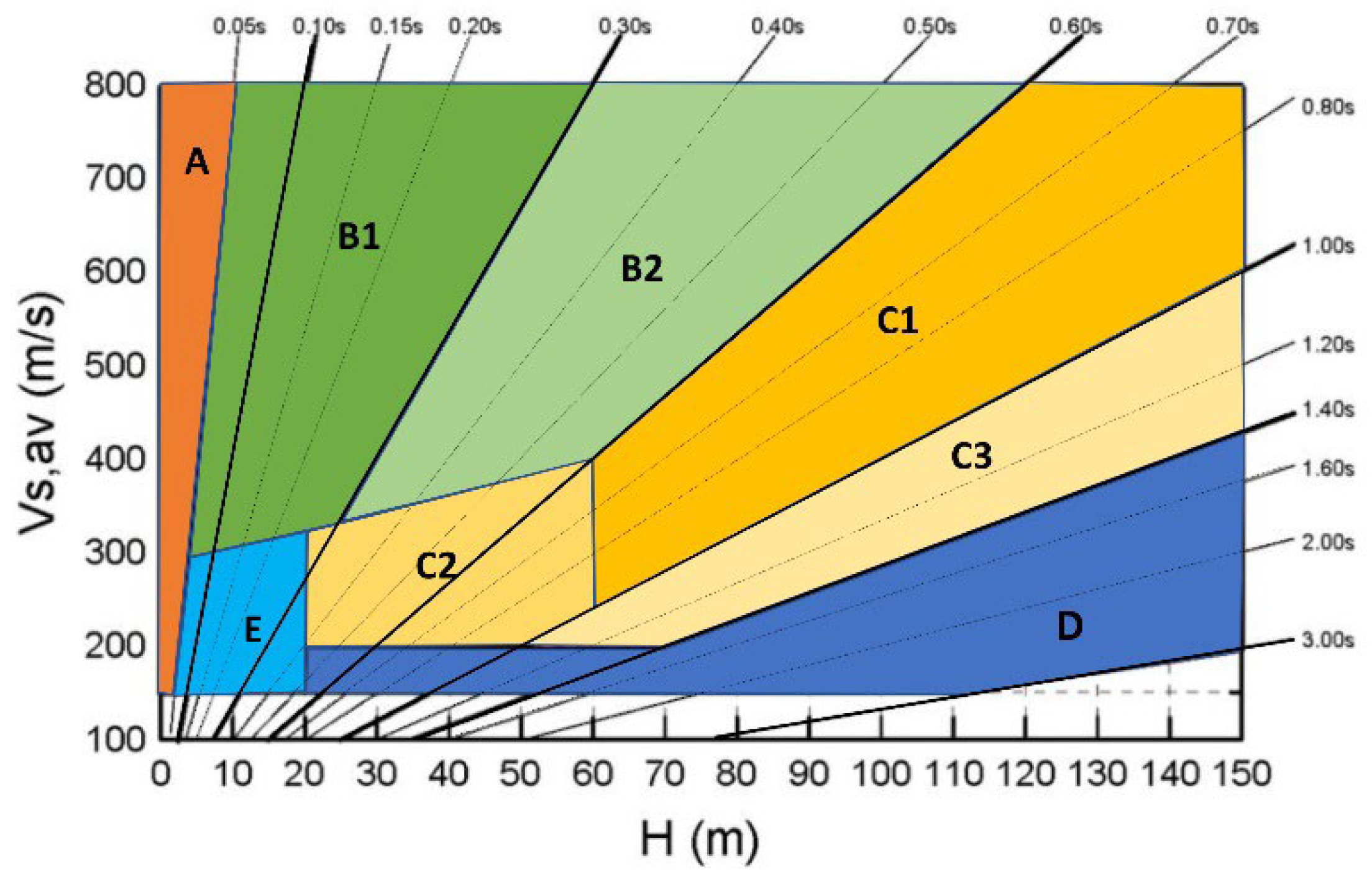
  149. Pitilakis, K.; Riga, E.; Anastasiadis, A.; Fotopoulou, S.; Karafagka, S. Towards the revision of EC8: Proposal for an alternative site classification scheme and associated intensity dependent spectral amplification factors. Soil Dyn. Earthq. Eng. 2019, 126, 105137. [Google Scholar] [CrossRef]
  150. Nakamura, Y. A Method for Dynamic Characteristics Estimation of Subsurface Using Microtremor on the Ground Surface; Railway Technical Research Institute: Tokyo, Japan, 1989. [Google Scholar]
  151. Costanzo, A.; Caserta, A. Seismic response across the Tronto Valley (at Acquasanta Terme, AP, Marche) based on the geophysical monitoring of the 2016 Central Italy seismic sequence. Bull. Eng. Geol. Environ. 2019, 78, 5599–5616. [Google Scholar] [CrossRef]
  152. Paolucci, R.; Faccioli, E.; Maggio, F. 3D Response analysis of an instrumented hill at Matsuzaki, Japan, by a spectral method. J. Seism. 1999, 3, 191–209. [Google Scholar] [CrossRef]
  153. Gallipoli, M.R.; Mucciarelli, M. Comparison of Site Classification from VS30, VS10, and HVSR in Italy. Bull. Seism. Soc. Am. 2009, 99, 340–351. [Google Scholar] [CrossRef]
  154. Ghofrani, H.; Atkinson, G.M.; Goda, K. Implications of the 2011 M9.0 Tohoku Japan earthquake for the treatment of site effects in large earthquakes. Bull. Earthq. Eng. 2013, 11, 171–203. [Google Scholar] [CrossRef]
  155. Ghofrani, H.; Atkinson, G.M. Site condition evaluation using horizontal-to-vertical response spectral ratios of earthquakes in the NGA-West 2 and Japanese databases. Soil Dyn. Earthq. Eng. 2014, 67, 30–43. [Google Scholar] [CrossRef]
  156. Field, E.H.; Zeng, Y.; Johnson, P.A.; Beresnev, I.A. Nonlinear sediment response during the 1994 Northridge earthquake: Observations and finite source simulations. J. Geophys. Res. 1998, 103, 26869–26883. [Google Scholar] [CrossRef]
  157. Schnabel, P.B.; Lysmer, J.; Seed, H.B. SHAKE: A Computer Program for Earthquake Response Analysis of Horizontally Layered Sites; University of California: Berkeley, CA, USA, 1972. [Google Scholar]
  158. Idriss, I.M.; Sun, J.I. User’s Manual for SHAKE91: A Computer Program for Conducting Equivalent Linear Seismic Response Analyses of Horizontally Layered Soil Deposits; Center for Geotechnical Modelling, Department of Civil and Environmental Engineering, University of California: Berkeley, CA, USA, 1992. [Google Scholar]
  159. National Cooperative Highway Research Program; Transportation Research Board; National Academies of Sciences; Engineering. Medicine, Practices and Procedures for Site-Specific Evaluations of Earthquake Ground Motions; The National Academies Press: Washington, DC, USA, 2012. [Google Scholar] [CrossRef]
  160. Kim, B.; Hashash, Y.M. Site Response Analysis Using Downhole Array Recordings during the March 2011 Tohoku-Oki Earthquake and the Effect of Long-Duration Ground Motions. Earthq. Spectra 2013, 29, 37–54. [Google Scholar] [CrossRef]
  161. Stewart Jonathan, P. Benchmarking of Nonlinear Geotechnical Ground Response Analysis Procedures; Pacific Earthquake Engineering Research Center: Berkeley, CA, USA, 2008. [Google Scholar]
  162. Huang, H.-C.; Huang, S.-W.; Chiu, H.-C. Observed Evolution of Linear and Nonlinear Effects at the Dahan Downhole Array, Taiwan: Analysis of the September 21, 1999 M 7.3 Chi-Chi Earthquake Sequence. Pure Appl. Geophys. 2005, 162, 1–20. [Google Scholar] [CrossRef]
  163. Arslan, H.; Siyahi, B. A comparative study on linear and nonlinear site response analysis. Environ. Geol. 2006, 50, 1193–1200. [Google Scholar] [CrossRef]
  164. Hosseini, S.M.M.M.; Pajouh, M.A. Comparative study on the equivalent linear and the fully nonlinear site response analysis approaches. Arab. J. Geosci. 2012, 5, 587–597. [Google Scholar] [CrossRef]
  165. Adampira, M.; Alielahi, H.; Panji, M.; Koohsari, H. Comparison of equivalent linear and nonlinear methods in seismic analysis of liquefiable site response due to near-fault incident waves: A case study. Arab. J. Geosci. 2014, 8, 3103–3118. [Google Scholar] [CrossRef]
  166. Civelekler, E.; Afacan, K.B.; Okur, D.V. Effect of site specific soil characteristics on the nonlinear ground response analysis and comparison of the results with equivalent linear analysis. J. Appl. Geophys. 2024, 220, 105250. [Google Scholar] [CrossRef]
  167. Basu, D.; Dey, A. Comparative 1D Ground Response Analysis of Homogeneous Sandy Stratum Using Linear, Equivalent Linear And Nonlinear Masing Approaches. In Indian Geotechnical Society, Kolkata Chapter Geotechnics for Infrastructure Development; Indian Geotechnical Society: Kolkata, India, 2016. [Google Scholar]
  168. Johari, A.; Heidari, A. Comparison of equivalent linear and nonlinear ground response analysis methods in the time domain. In Proceedings of the 3rd National & 1st International Conference in Applied Research on Civil Engineering, Architecture and Urban Planning, Compiegne, France, 28–30 June 2020; pp. 1–7. [Google Scholar]
  169. Assimaki, D.; Li, W. Site- and ground motion-dependent nonlinear effects in seismological model predictions. Soil Dyn. Earthq. Eng. 2012, 32, 143–151. [Google Scholar] [CrossRef]
  170. Kumar, S.S.; Dey, A.; Krishna, M. Equivalent linear and nonlinear ground response analysis of two typical sites at Guwahati city. In Proceedings of the Indian Geotechnical Conference IGC-2014, Kakinada, India, 18–20 December 2014. [Google Scholar]
  171. Locat, J.; Beauséjour, N. Corrélations entre des propriétés mécaniques dynamiques et statiques de sols argileux intacts et traités à la chaux. Can. Geotech. J. 1987, 24, 327–334. [Google Scholar] [CrossRef]
Figure 1. Schematic representations of the main amplifying effects in soft soil: (a) broadband amplification, (b) resonance effect, (c) buried valley focusing effect, and (d) basin-edge effect.
Geosciences 15 00128 g001
Figure 2. Amplification of soil models for periods 0.001 to 10 s as a function of Tosc and T0 [24,25].
Geosciences 15 00128 g002
Figure 3. Models of site amplification in the Seattle Basin, Washington State, illustrating resonance and broadband amplification effects: (a) single-layered and (b) four-layered (Modified from [29]).
Geosciences 15 00128 g003
Figure 4. Topographic amplification effect on a gentle slope: (a) Effect of slope angle (modified from [35]) (b) Effect of slope curvature (modified from [36]).
Geosciences 15 00128 g004
Figure 5. Amplification of local seismic events by the Seattle Basin, Washington State (a) amplification for waves of different frequencies along horizontal distance (b) geological cross-section of the basin (Modified from [29]). Stars denote the stations that contribute to the higher plots.
Geosciences 15 00128 g005
Figure 6. Suspension Logging Test (a) crosshole test (b) downhole test (c) uphole test (modified from [46]).
Geosciences 15 00128 g006
Figure 7. Flowchart of the procedure for the SPAC methodology (Modified from [64]).
Geosciences 15 00128 g007
Figure 8. Normalized stiffness degradation curve (modified from [81]).
Geosciences 15 00128 g008
Figure 9. Stress–strain behavior in dynamic loading (a) complete hysteresis loop with loading and unloading (b) loading curve only with failure stage (Modified from [6]).
Geosciences 15 00128 g009
Figure 10. Concept for the use of seismic piezocone pressure meter test with dissipation phase for site exploration (modified from [84]).
Geosciences 15 00128 g010
Figure 11. Cyclic relations for (a) shear modulus (SM) and (b) damping ratio (DR) curves for sandy soils (after [91]).
Geosciences 15 00128 g011
Figure 12. Cyclic relations for (a) shear modulus (SM) and (b) damping ratio (DR) curves for clayey soil (OCR 1–15) (after [97]).
Geosciences 15 00128 g012
Figure 13. Cyclic relations for (a) shear modulus (SM) and (b) damping ratio (DR) curves for eastern Canadian sensitive clay (after [101]).
Geosciences 15 00128 g013
Figure 14. Nonlinear effect in dynamic loading for different types of soil: (a) reduction of PGA on soft soils for destructive earthquakes (modified from [12]) (b) Spectral acceleration at the surface vs. the vibration period from a statistical analysis of 104 strong-motion records (modified from [104]).
Geosciences 15 00128 g014
Figure 15. Probabilistic seismic hazard analysis (PSHA): (a) study area with nearby sources, (b) earthquake occurrence (Guttenberg–Richter relation), (c) ground motion prediction equations (GMPE), (d) ground motion hazard curve that describes the probability of exceedance of a given level of the selected shaking intensity measure.
Geosciences 15 00128 g015
Figure 16. 5% damped response spectra of selected ground motions matching target spectrum with different techniques (a) scaled linearly with a constant factor, (b) conditional mean spectrum (CMS), and (c) modified in the frequency domain (modified from [122,124]).
Geosciences 15 00128 g016
Figure 17. Site amplification empirical models as a function of VS30 (a) for 0.2 s period (b) for 1.0 s period [132,133,134,135,136] (Modified from [132]).
Geosciences 15 00128 g017
Figure 18. Comparison of T0 of soil in different methods.
Geosciences 15 00128 g018
Figure 19. Correlation of H with Vsavg and T0 for the site classes A through E (Modified from [149]).
Geosciences 15 00128 g019
Figure 20. Comparison of H/V ratio (a) based on site class from NEHRP (b) based on Vs30 (modified from [156]).
Geosciences 15 00128 g020
Figure 21. Slope Geometry of the 2D Model for Dynamic FEM Analysis.
Geosciences 15 00128 g021
Figure 22. (a) Input Earthquake Motion; (b) Amplification Curves at Different Points on the Surface of the Slope Model.
Geosciences 15 00128 g022
Figure 23. Maximum Horizontal Displacement of the Slope Model After Dynamic Loading.
Geosciences 15 00128 g023
Table 1. Empirical correlations of Vs with CPT parameters (after [47]).
CorrelationSoil TypeReference
Vs = [ 10 0.55 I c + 1.68 ( q t σ v o P a ) ] 0.5All Soils[49]
Vs = 1.75   q c 0.627 Clayey Soil
Vs = 155   q c 0.29 f s 0.10 Clayey Soil[50]
Vs = 224   q c 0.26 f s 0.01 Sandy Soil
Vs = 0.0831 Qtne1.786Ic ( σ o P a ) All Soils[51]
Vs = 2.27   q t 0.412 I c 0.098 Z 0.033 All Soils[52]
Vs = 2.934   q t 0.395 I c 0.912 Z 0.124 All Soils
Vs = 1.961   q t 0.579 (1 + Bq)1.202Marine Clay Soil[53]
Vs = 10 ( 0.8 I c 1.17 ) Q tn Silty Soil[54]
Vs = 18.4   q c 0.144 I c 0.0832 Z 0.278 Sandy Soil[55]
Vs = 39   q t 0.164 Z 0.137 Sandy Soil[56]
Vs = 8.35   ( q t σ v o ) 0.22 σ v o 0.357 Marine Clay[57]
Vs = 43.7   ( Q t n 0.25 D 50 0.215 ) Clayey Soil[58]
Vs = 71   ( Q t n 0.25 D 50 0.1 ) Sandy Soil
Vs = 35.1   q t 0.188 f s 0.102 Z 0.139 Silt and Sand mixtures[59]
Vs is shear-wave velocity, Ic is soil behavior type index, σνo is overburden stress, qc is raw cone tip resistance, qt is corrected cone tip resistance, Z is depth, Bq is normalized pore pressure, Qtn is normalized cone resistance, D50 is effective mean diameter, and fs is sleeve friction resistance.
Table 2. Advantages and Disadvantages of in-situ methods of measuring shear-wave velocity.
MethodAdvantagesDisadvantages
Seismic Reflection
Provides detailed imaging of subsurface layers.
Can explore deeper depths.
Cost-effective and easy to use.
Non-invasive.
Not a direct calculation method of Vs
Requires advanced processing and interpretation skills.
Seismic Refraction
Cost-effective for thinner stratigraphy.
Easy to deploy in suitable conditions.
Non-invasive.
Not a direct calculation method of Vs.
Limited to increasing velocity layers.
Less effective for complex subsurface or thin layers.
MASW
Probes deeper depths with good resolution.
Suitable for large-scale surveys.
Provides detailed imaging of Vs along the array.
Cost-effective and easy to use.
Non-invasive.
Not a direct calculation method of Vs.
Requires more equipment and computational effort.
Sensitive to noise and ground coupling issues.
SASW
Simple setup and cost-effective.
Effective for shallow investigations.
Non-invasive.
Not a direct calculation method of Vs.
Limited depth penetration.
Lower resolution compared to MASW for deeper layers.
Suspension Logging
Accurate measurements of Vs along the depth.
Invasive and costly.
Challenging to weather and other site conditions.
Requires suitable borehole conditions.
Seismic Cone Penetration Test (SCPT)
Provides both geotechnical and dynamic properties.
High accuracy for Vs measurement.
Reliable in soft soils.
Invasive and site-dependent.
More expensive than non-invasive methods.
Requires skilled operation.
Table 3. Standard site classification schemes according to the NBCC and Eurocode 8.
CodeSite Class and Vs30 (m/s)
ABCDE
NBCC (NEHRP)>1500 (*)760–1500 (*)360–760180–360<180
Eurocode 8>800 (**)360–800180–360<180(***)
* Soft Soil must be <3 m in thickness; ** Surface weak materials must be <5 m; *** Vsavg < 360 m/s and thickness 5 < H < 20 m.
Table 4. Representative Techniques for Determining the Fundamental Period from Soil Profiles (modified from [143]).
NumberEquationVelocity ModelMethod NameReferences
1T = 4 H V s Single LayerConstant Distribution of Shear-Wave Velocity with Depth[141,144]
2T = 4 i = 1 n ( h i V i ) Multiple Layer
3T = π i = 1 n ( h i V i ) Single Layerπ times the VS travel time method (Wang et al., 2018)[143]
4 a 1 = 2 z 1 2 ln H z 1 1 H 2 z 1 T t H ; b 1 = 2 l n ( H z 1 1 ) T t ( H )
μ = V ( H ) V ( 0 ) = 1 + b 1 H a 1
T = 4 H a 1   1 0.206 + 0.798 µ 1 0.853 For μ1 > 1
T = 4 H a 1   1 0.0715 + 0.928 µ 1 0.750 For μ1 ≤ 1
Single LayerLinear Distribution of Shear-Wave Velocity with Depth (Deposit with V = a1 + b1z)[139]
5 a 2 = ln H z 1 H l n 2 l n ( H z z ) T t H ; b 2 = ln H 2 z 1 ln H z 1
T = 4 H a 2 H b 2 1 0.25 b 2 2 0.34 b 2 + 1 for 0 ≤ b2 < 0.875
T = 4 H a 2 H b 2 1 4.1 b 2 2 + 6.4 b 2 + 1.958 for 0.875 ≤ b2 < 0
Single LayerPower-Law Distribution of Shear-Wave Velocity with Depth
(Deposit with V = a2 zb2)
[82,144]
6a3 = ( 4 z 2 H T t H ) 2 ; b3 = 8 ( H 2 z 1 ) T t H 2
μ3 = V ( H ) V ( 0 ) = 1 + b 3 H / a 3
T = 4 H a 3 0.5 1 0.280 + 0.719 µ 3 0.960 for 0 ≤ μ3 < 1
T = 4 H a 3 0.5 1 0.303 + 0.691 µ 3 1.031 for μ3 > 1
Single LayerLinear Distribution of Shear Modulus with Depth
(Deposit with V = (a3 + b2z)0.5)
[140,141]
7Ta−b =
Ta π 2 8 [ 0.75 + T b T a 2 1 + 2 h a h b ]
for Tb/Ta > 0.1, ha > hb
Ta [1 + β T b T a k 1 + h a h b k ]1/k
for Tb/Ta > 0.1, ha ≤ hb
Ta [1 + h a h b T b T a 2 ]
for Tb/Ta ≤ 0.1
Here,
β = 1 − 0.2 (ha/hb)2 and k = 4 − 1.8 (ha/hb)
Approximate Madera model[142]
8 T a = 4 d a V s a ; T b = 4 d b V s b
tan( π 2   T a T a b ) tan( π 2   T b T a b ) =
Multiple LayerSuccessive application of two layers[142]
9Xi = 0; Xi+1 + (H − Hmi) h i V i 2
T = π i = 1 n ( X i + X i + 1 ) 2 h i i = 1 n ( X i + X i + 1 ) 2 h i v i 2
Multiple LayerSimplified Rayleigh method[144]
10T = 2π D 3 3 i = 1 N V s i 2 d i Multiple LayerLinear fundamental Mode Shape[144]
11T = i = 1 n ( 4 h i V i ) 2 2 H m i h i Multiple LayerJapanese seismic design code (BCJ) method[145]
μ1 =bottom-to-surface velocity ratio, H = soil depth, Tt = the travel time from surface to bedrock, z1 = depth corresponding to half of the travel time, Hmi = depth of midpoint of the ith soil layer, 4hi/Vi = the fundamental period of the ith layer, and 2Hmi/hi = weight value determined by the depth and thickness of the ith layer.
Table 5. Site classification based on fundamental site period and corresponding NEHRP site classes. (After [149]).
Site ClassDescriptionSite PeriodNEHRP Site Class
Hard Rock A
SC IRockTo < 0.2 sA + B
SC IIHard Soil0.2 ≤ To < 0.4 sC
SC IIIMedium Soil0.4 ≤ To < 0.6 sD
SC IVSoft SoilTo ≥ 0.6 sE + F
Table 6. Advantages and shortcomings between linear, equivalent linear, and nonlinear analyses.
AdvantagesLimitations
Linear
Requires less time.
Requires fewer input parameters.
Simple methodology.
Produces satisfactory results for stiff soil and low-frequency ground motion.
No need for nonlinear soil curves.
Unable to capture nonlinear soil behavior or provide hysteresis curves due to earthquake motion
Unsatisfactory results for soft soil and high-frequency ground motion
Analysis confined to specific strain ranges
Equivalent linear
Requires less time
Simple methodology
Yields comparable results to nonlinear analysis within specific frequency ranges
Unable to capture nonlinear soil behavior or provide hysteresis curves during earthquake motion
Results may vary compared to nonlinear analysis for high-frequency ranges
Analysis is restricted to specific strain ranges
Nonlinear
Captures nonlinear soil behavior and provides hysteresis curves during earthquake motion
Offers real stress–strain curves and information on pore pressure buildup
Analysis feasible for any strain range
Suitable for all types of soil and ground motion intensity
Requires more time
Requires more input parameters
Demands precise and in-situ nonlinear soil curves (shear modulus and damping ratio)
Disclaimer/Publisher’s Note: The statements, opinions and data contained in all publications are solely those of the individual author(s) and contributor(s) and not of MDPI and/or the editor(s). MDPI and/or the editor(s) disclaim responsibility for any injury to people or property resulting from any ideas, methods, instructions or products referred to in the content.

