2.1. Study Area
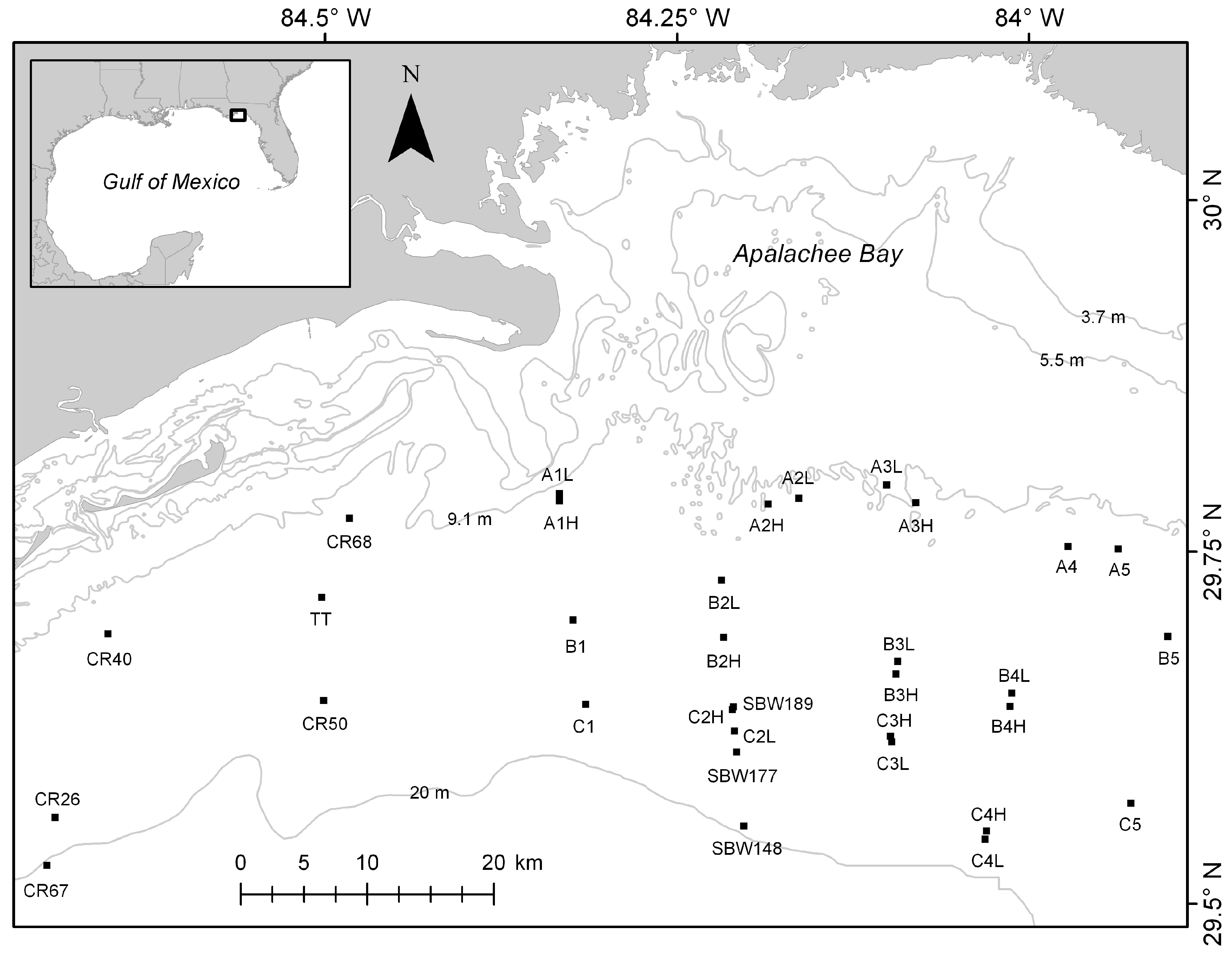
The location of this study was the nearshore marine areas of the Northeastern Gulf of Mexico off the coast of Northwest Florida (
Figure 1). The seafloor in this region is primarily drowned karst with sand, limestone, and detrital sediments [
12]. The continental shelf is wide (up to 188 km across) and gently sloped [
12]. Currents, fronts, and waves affect the region at a variety of temporal scales from hourly changes from semi-diurnal tidal currents to the occasional storm surge that accompanies tropical systems that hit the area on an annual, or longer time scale.
Nearshore benthic habitats generally consist of sand and limestone hardbottom. Hardbottom refers to rocky substrate or consolidated sediments that are often exposed, but can be covered with a veneer of sand. Pavement, ledges, outcrops, and karren are different forms of hardbottom found here and provide substrate for a large variety of sessile invertebrates and algae to attach. For this reason, hardbottom is also often referred to as ‘live bottom’. Common sessile inhabitants are sponges, hard corals, ascidians, bryozoans, bivalves, hydroids, gorgonians, and algae. These organisms provide additional structure for motile invertebrates and fishes to use as shelter. Hardbottom habitats have high biodiversity particularly as compared to surrounding sand habitat. They are also home to many important fisheries species including gag, Mycteroperca microlepis, red grouper, Epinephelus morio, gray snapper, Lutjanus griseus, and stone crabs, Menippe mercenaria. People visit hardbottom habitats within the study area for recreational fishing and SCUBA diving. Commercial fishermen also frequent these areas to fish, trawl for shrimp, and collect sponges.
2.2. Methodology
Thirty-three sites were visited between February and December 2011 (
Figure 1). Several of these sites were visited seasonally or on more than one occasion. Sites were chosen from known or suspect hardbottom locations. All 33 sites were mapped using a Humminbird 997c sidescan sonar system (Humminbird, Eufaula, AL, USA) operating at 455 kHz with a 100 m swath width and 25% overlap of the tracks to cover an area approximately 400 m × 400 m. When time was available sites were mapped in both the north-south and east-west directions. If time was limited the mapping direction was determined based on the wind and wave conditions and which would yield the highest quality imagery. The tracks were imported into Chesapeake Sonarwiz.Map (Chesapeake Technology, Inc., Mountain View, CA, USA) and a mosaic was made for each site using the best available imagery. Each mosaic was exported as a geotiff and then manually delineated into the acoustic classes of hardbottom (“pavement area”/“rock substrate” according to the CMECS [
3]) and sand in ESRI ArcMap 10.0 (Environmental Systems Research Institute, Inc. (ESRI), Redlands, CA, USA). Manual classifications were done at 1:700 scale. Kendall et al. [
13] used a comparable scale of 1:1000 to manually delineate similar habitat classes. The distance from each 400 m
2 site to the closest point on shore was also measured in ArcMap. For additional details on the sidescan sonar mapping and post-processing procedures see Kingon [
14].
During the site visits, dive surveys were also performed and consisted of taking measurements along two 15 m transects. Both transects originated from an anchor with an attached surface buoy that was dropped from the vessel on the site coordinates. Transects were run following randomly-selected headings. If, after 10 m, hardbottom habitat was no longer present, then an alternate random heading was used. Along each transect, rugosity measurements were made every 3 m using a 3 m weighted line draped along and following the contours of the bottom parallel to the transect tape. The transect tape was then used to measure the straight-line distance from the start of the rugosity line to the end. Rugosity was calculated by dividing the length of the weighted rugosity line (3 m) by the recorded straight-line distance. Video footage was taken along each transect using a Canon PowerShot S90 digital camera in a Canon WP-DC35 underwater housing (Canon U.S.A., Inc., Melville, NY, USA) for categorizing fine-scale geoforms, relief and heterogeneity (patchy, continuous, or mixed patchy/continuous). Geoforms were assigned using the CMECS as sediment sheet, ripples, pavement area—smooth, pavement area—rough, pavement area—slabs, karren—slabs with sand channels, ledge—no overhang, ledge—with overhang, or rock outcrop. Relief classes ranged from very low where sites had almost no relief to high at sites with features over 1 m tall. The other classes ranked in between the two accordingly (low, medium, and medium/high). These same classes for geoform, relief and heterogeneity were also assigned to the sidescan sonar imagery for the entire mapped area.
Additionally, along each transect, point measurements were made every 1.5 m. At each point, a measuring probe was inserted into the sediment to measure the sediment depth. The sediment depths were later categorized into no sand, dusting (<1 cm), thin sand (1–5 cm), and thick sand (>5 cm) classes. At that same point along the transect lines, all epibiota in contact with the probe were identified and their heights from the surface measured. Epibiota included any macrofauna/flora (>1 to 3 cm) and large megafauna/flora (>3 cm) that were attached to the substrate or that moved slowly enough that they were considered sedentary. Taxa were not identified to genus or species level for this study because the scientific divers who assisted with the dive surveys had various backgrounds from undergraduates to experts in topics such as oceanography and fisheries. Therefore, taxa were assigned to easily identifiable groups, see
Table 1, and these categories covered all the organisms encountered. Point surveys were done to save time underwater on SCUBA, which was further limited at some sites by depth and seasonally by temperature. These surveys were conducted in conjunction with other research, which also restricted the time available.
Next if there were any rocks within a 1 m radius of the probe, the height of the closest one was measured. Expanding the measuring area for rock height beyond a single point allowed the acquisition of more rock heights. At a single point, it was unlikely that the probe location would be right next to the vertical dimension of a rock. This method allowed rock heights to be measured even if the probe landed on top of or near rocks. A rock sample was collected from each site using a hammer and chisel to break off a large piece of the bedrock. The rock samples were first sent to geologist Dr. Kathy Scanlon at the USGS (United States Geological Survey), Science Center for Coastal and Marine Geology in Woods Hole, Massachusetts for analysis. Then they were brought to geologist Harley Means at the Florida Geological Survey in Tallahassee, Florida for confirmation and to be archived in their collection. Rock descriptions included rock type, reaction to 10% hydrogen chloride (HCl), color, hardness, density, presence of corals and fossils, degree of bioerosion, and recrystallization, and presence of quartz sand. For the classification, I only used rock type and rock reaction to HCl as the other parts of the descriptions were more subjective and difficult to categorize. Rock type was assigned as either dolostone, limestone, non-rocks/biogenic formations, or unknown. Reactions to HCl were classified as strong, weak, or no reaction.
Divers also recorded underwater visibility, depth, and temperature. Horizontal visibility was measured by noting the distance on the transect tape when the anchor became almost out of sight. Vertical visibility was recorded on ascent (using the diver’s depth gauge) as the depth at which the bottom was barely visible, similar to a secchi disk measurement without having to carry an extra piece of equipment on every dive. A small Sensus Ultra recorder (ReefNet Inc., Mississauga, ON, Canada) was clipped to a diver during each dive that recorded water depth and temperature at 10-second intervals. The maximum depth, average bottom temperature, and average surface temperature were extracted from these files for each dive.
The temperature regime was calculated by averaging the temperatures recorded across sites for each season, and then averaging the seasonal means to derive a mean annual temperature. Sampling effort differed between seasons primarily due to inclement weather conditions, so calculating annual temperature in this manner helped account for those differences (winter: n = 15; spring: n = 18; summer: n = 27; fall n = 12).
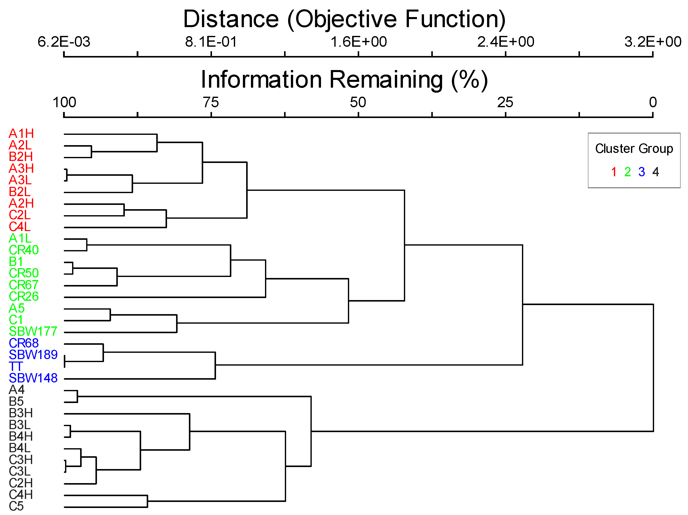
Using the dive survey transect data, I calculated percent covers and height/depth summary statistics for the rocks, sand, and epibiota at each site. This was done by dividing the number of occurrences of each by the number of points surveyed along each transect and then the percent covers for the two transects at each site were averaged together. The percent cover taxa data at each of the 33 sites was input into a two-way cluster analysis in PC-ORD, version 5 (MjM Software, Gleneden Beach, OR, USA) [
15]. A Sorensen (Bray-Curtis) distance measure was chosen and the Flexible Beta group linkage method with the beta value set to −0.25 was used. The data were relativized by dividing each column value by that column’s maximum value. This method of clustering is space conserving and works with nonparametric data [
15]. The two-way analysis provided site groupings based on their taxa. To see which taxa were driving the cluster groupings, a species indicator analysis and a species indicator Monte Carlo randomization test using 1000 permutations were also run in PC-ORD.
Using the sidescan sonar data and the dive survey measurements, I implemented the CMECS. I first used general information about the region to assign the biogeographic and aquatic settings. Then, using the four components (water column, geoform, substrate, and biotic), I classified the nearshore benthic characteristics within the study area to the finest scale possible. The general hierarchical classification template within each component for the CMECS was enhanced with modifiers when appropriate. Modifiers are not required, but provide a means for describing the CMECS units in greater detail and for inserting other pertinent information [
3]. Two commonly used modifiers are co-occurring elements and associated taxa [
3]. Co-occurring elements are often used when more than one CMECS unit is needed to appropriately describe a habitat, e.g., if there is more than one dominant substrate type or biotic class [
3]. Associated taxa are biota that are capable of moving between habitats, but are commonly seen at the habitat being classified [
3]. These were not included in this paper. Other modifiers include seafloor rugosity, temporal persistence, turbidity, and photic quality (see FGDC [
3] for more details on modifiers). Photic quality is a broad scale classifier and does not address light levels, mostly just presence/absence so, instead, the turbidity modifier classes were assigned based on the visibility methods discussed above. When it was deemed necessary, slight deviations from the CMECS protocol were implemented.


