Article

The Role of Shear Wave Velocity and Non-Linearity of Soil in the Seismic Response of a Coupled Tunnel-Soil-Above Ground Building System

by
Glenda Abate
*,
Salvatore Grasso
and
Maria Rossella Massimino
Department of Civil Engineering and Architecture, University of Catania, Piazza Università, 95124 Catania, Italy
*
Author to whom correspondence should be addressed.
Geosciences 2019, 9(11), 473; https://doi.org/10.3390/geosciences9110473
Submission received: 27 September 2019 / Revised: 19 October 2019 / Accepted: 25 October 2019 / Published: 9 November 2019
(This article belongs to the Special Issue Seismic Sequence in Mediterranean Region)

Abstract

:
The presence of tunnels close to aboveground structures may modify the response of these structures, while the contrary is also true, the presence of aboveground structures may modify the dynamic response of tunnels. In this context, the dynamic properties of the soil through which the aboveground and underground structures are “connected” could play an important role. The paper reports dynamic FEM (Finite Element Method) analyses of a coupled tunnel-soil-above ground structure system (TSS system), which differ in regards to the soil shear wave velocity and in turns for the damping ratio, in order to investigate the role of these parameters in the full-coupled TSS system response. The analyses were performed using three different seismic inputs. Moreover, the soil non-linearity was taken into account adopting two different constitutive models: i) an equivalent linear visco-elastic model, characterized by degraded soil shear moduli and damping ratios, according to suggestions given by EC8 in 2003; and ii) a visco-elasto-plastic constitutive model, characterized by isotropic and kinematic hardening and a non-associated flow rule. The seismic response of the system was investigated in the time and frequency domains, in terms of: acceleration ratios; amplification ratios and response spectra; and bending moments in the tunnel.

1. Introduction

Currently, it is becoming ever more evident that there is a growing need for tunnels, in order to solve the problems faced by transportation and utility networks. In seismic areas, it is extremely important to assess the possible damage to the tunnel and to the aboveground structures as a result of earthquakes. Historically, tunnels have experienced a lower rate of damage than aboveground structures [1]. Nevertheless, recent studies have documented significant damage suffered by tunnels due to seismic events [2,3,4,5,6]. During an earthquake, the vibrations of aboveground structures may modify the dynamic response of tunnels [7,8]; at the same time, the presence of shallow tunnels may alter the response of aboveground structures. Most of the published papers consider only tunnel-soil systems [9,10,11,12,13,14,15], while a few consider tunnel-soil-aboveground structure systems (TSS systems) [16,17,18,19,20].
In TSS system behavior a fundamental role is played by dynamic soil parameters, and particularly by the shear wave velocity VS and damping ratio D of the soil through which the seismic waves move and which connects the tunnel to the aboveground structures. Currently, it is possible to accurately estimate VS and D directly or indirectly by means of a number of in-situ and/or laboratory tests [21,22,23]. Nevertheless, given the considerable extension of tunnels, it is economically very expensive to accurately estimate these parameters for tunnels. This very often leads to unavoidable approximation in the evaluation of VS profiles along the vertical and horizontal directions. It is then very interesting to investigate the effects of VS and D on the evaluation of the seismic response of TSS systems.
The present paper deals with parametric analyses performed by means of FEM modeling and involving a TSS system, with differing VS profiles and D, in order to underline the role of estimating these parameters. Using the case history of the underground network in Catania (Italy) and taking a cross-section including an aboveground building [20], the real VS profile [21] was modified according to the four soil types reported by the Italian Technical Code [24].
The analyses were performed in 2-D, considering the transversal direction of the tunnel, because the ovaling or racking deformations of tunnels are generally the most dangerous under seismic loading [9,25]. Isotropic visco-elastic-linear behavior was assumed for the tunnel and the aboveground structures. In order to take soil non-linearity into account, two different constitutive models were adopted for the soil: i) an equivalent linear visco-elastic model, characterized by degraded soil shear moduli G and damping ratios D, depending on the expected peak horizontal acceleration (PHA) at the ground surface according to suggestions given by [26]; and ii) a visco-elasto-plastic constitutive model, characterized by isotropic and kinematic hardening and a non-associated flow rule [
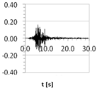
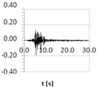
27,
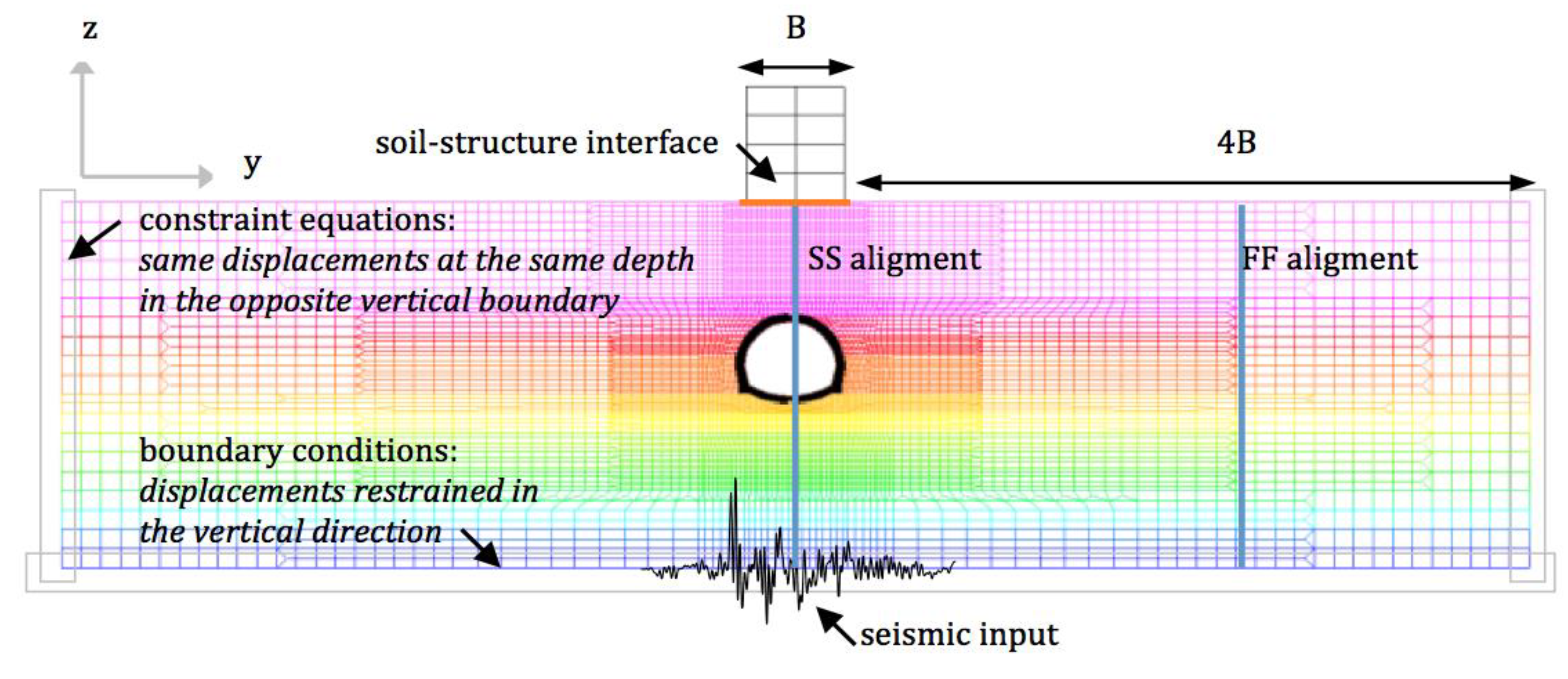
28]. Finally, three different seismic inputs were applied at the base of the models.
The seismic response of the TSS system was investigated in the time and frequency domains, in terms of: amplification ratios along the symmetry axis of the building and of the tunnel (SS alignment) and along a parallel alignment in free-field conditions (FF alignment); and bending moments in the tunnel. The latter were also compared with those obtained using the closed-form solutions by [29] and [30].
The paper highlights the importance of the investigation of Vs profiles in the study of the seismic response of TSS systems. Some interesting considerations on simplified versus sophisticated methods for taking into account soil nonlinearity have been developed.

2. The TSS System Investigated

The benchmark of the FEM analyses was a cross-section of the Catania (Italy) underground system actually under construction. The section includes an aboveground building (Figure 1 and Figure 2) [20]. The geotechnical characterization of the soil, performed in two different phases (July 1999 and December 2005–January 2006), shows the soil profile reported in Figure 1 and is characterized by a silty clay (ALg) and a clay (Aa) sub-lithotypes, which belong to the same lithotype, whose Young’s modulus Es0 is constant for the first 10 m at a very small-strain and then increases linearly with depth (in the 300–1700 MPa range) and whose unit weight (γ) is equal to 20 kN/m3. No ground water table is present. Therefore, according to [24], the soil can be classified as type C.
The cross-section is characterized by a reinforced concrete building 10 m wide, with two equal spans in the direction under investigation, and 12 m high, with four levels and shallow foundations, whose properties are: Eb = 28,500 MPa, νb= 0.2, γb = 25 kN/m3; and Db = 5%. The reinforced concrete tunnel is 11 m wide and 7.2 m high, with a horseshoe section, and it is located 18 m below the ground surface. Its properties are the same as the reinforced concrete building: E1 = 28,500 MPa, ν1 = 0.2, and Dl = 5%.
Using this case-history as a basis, different parametric analyses were carried out varying the VS, choosing average values within the ranges provided by [24] for the four types of soil classified as A, B, C, and D. The values adopted for VS for each type of soil, as well as the corresponding stratigraphic amplification factor SS provided by [24] and evaluated for Tr = 475 years, are shown in Table 1.

3. FEM Modeling

3.1. General Information

The seismic response of the TSS system described in Section 2 was modeled by the ADINA code [31,32], widely used by the authors in dynamic analyses [15,33,34,35,36,37]. Figure 2 shows the mesh used, including the boundary conditions and the seismic input at the base of the model (bedrock). Moreover, the two parallel alignments in which the response of the system was analyzed, one along the symmetry axis of the building and of the tunnel (SS alignment) and another one in free-field conditions (FF alignment), are also represented in Figure 2 as blue lines. The width of the soil deposit was fixed equal to 150 m (>4B, where B is the width of the building), in order to avoid boundary effects as far as possible; the height of the soil deposit derives from geotechnical investigations according to which the bedrock was found at a depth of 38 m. The nodes of the soil vertical boundaries were linked by “constraint equations” that impose the same displacements at the same depth [33,36,38,39,40]. All the nodes of the base of the mesh were restrained in the vertical direction. The mesh element size was chosen in order to ensure the well-known condition hVs,min/6 ÷ 8 fmax [41], being h the maximum element size and fmax the maximum frequency of the system. Moreover, a finer discretization was adopted near the tunnel and the aboveground structure. In order to model probable uplifting and/or sliding phenomena, special contact surfaces were used between the soil and the aboveground structure, considering a friction equal to 2/3 φ. Tunnel-soil slip was not allowed [25].
Rayleigh damping factors αr and βr were computed according to the well-known relations [42,43,44,45]: αr = Dω and βr = D/ω, being D the damping ratio and ω the angular frequency of the systems involved. More precisely, different values of αr and βr were computed for the tunnel, the soil and the building according to their different D values for the tunnel. The angular frequency ω was evaluated according to the first fundamental periods of the soil, the tunnel and the building, (ω = 2π/T). The first fundamental period of the building was evaluated according to the Italian Technical Code [46]: for civil or industrial buildings that do not exceed 40 m height and whose mass is approximately distributed along the height, the period can be estimated as Tb = C1 hb3/4, with hb = height of the building, in meters, from the foundation level; C1 = 0.075 for buildings with reinforced concrete frame structures. According to [47] the first fundamental period of the soil is Ts = 4H/Vs,av, in which Vs,av is the average value of Vs from the bedrock to the soil surface. Finally, the first fundamental period of the tunnel was assumed equal to that calculated for the soil, because the tunnel and the soil, being closely related, typically respond similarly to the movement induced by the earthquake.
The tunnel and the building were modeled by 2-node beam elements, adopting a linear visco-elastic constitutive model. The soil was modeled by 9-node solid elements and by two different constitutive models, described in the following Section 3.2 and Section 3.3.
Three seismic inputs were used (Table 2): they differed in regards to frequency content and were scaled at the same two different ag: 0.1 g and 0.3 g, which were chosen with reference to the two "limit" values proposed by [26] in relation to which the shear modulus G and the damping ratio D have to be degraded to take the soil non-linearity into account (Table 3).

3.2. Equivalent Linear Visco-Elastic Modeling

Firstly, the soil was modeled by an equivalent linear visco-elastic model; it was characterized by constant reduced G and increased D, modified in line with [24], i.e., with reference to the expected PHA at the ground surface, equal to SSag (Table 3). In effect, [24] gives suggestions for soil type D; proportionally similar assumptions were adopted for the other soil types.
Therefore, eight different complete 2-D FEM models were defined for the equivalent linear visco-elastic analyses, distinguished on the basis of a different combination of the two parameters: Vs profile (and therefore soil type) and seismic input. The fourth and fifth columns of Table 4 show the seismic parameters D and G adopted (indicated as "operative" values). They were modified as suggested by [26], taking into account SS (Table 1) and the fixed ag.

3.3. Non-Linear Visco-Elastic Modeling

The second constitutive model adopted [27,28] was an elasto-plastic constitutive model, including isotropic and kinematic hardening, based on the Mohr–Coulomb failure criterion and a non-associated flow rule, named the Severn-Trent model. Moreover, it allows us to analyze soil softening and/or hardening. In particular, given the complexity of the non-linear model, only two different values of VS were taken into account, corresponding to the two soil types, B and C. Therefore, these two different soils were modeled using the Severn-Trent constitutive model, considering the two different ag adopted (0.1 g and 0.3 g). Therefore, in total four case studies were analyzed, called B1 or B2 and C1 or C2 (Table 5).
Table 5 also shows the values used to model the soil types B and C for the non-linear analyses. The Severn-Trent constitutive model is characterized by ten parameters: the elastic parameters E and ν were set according to Section 2; the parameters vλ, λ and ϕcv (of the critical state) were obtained starting from the results of the laboratory tests carried out on the real reference deposit; the parameters R, A, kd, B, and k (size of kinematic yield surface, dilatancy parameters, distortional strain hardening parameter, and effect of state parameter on strength) were derived from values in literature [27]. Finally, the soil damping ratio was fixed according to [26] (see Table 4).

4. Results of the Equivalent Visco-Linear Elastic Analyses

This section reports the results obtained performing the equivalent visco-linear elastic analyses discussed in Section 3.2. They are expressed in terms of: (1) the acceleration amplification ratio Ra, which is the ratio between the maximum acceleration at a given point and the maximum acceleration at the bedrock. This ratio was analyzed for the SS alignment and for the FF alignment (Figure 2); (2) the soil amplification function for the two SS and FF alignments: this is the ratio between the Fourier spectrum at the surface and the Fourier spectrum at the bedrock; (3) the surface response elastic spectrum in SS, compared with that provided by the Italian Technical Code [24]; and (4) the seismic bending moments in the tunnel (in the transverse section per unit of longitudinal dimension), evaluated for four specific points on the contour of the tunnel(θ = 45°, θ = 135°, θ = 225°, and θ = 315°).

4.1. Response in the Time Domain

4.1.1. Amplification Ratio in the Soil

Figure 3 shows the comparison, for the same soil type and considering the variation of the seismic input, between the amplification ratio along the SS alignment (continuous lines) and the FF alignment (dashed lines); furthermore, the values of the stratigraphic coefficient SS provided by [24] have been reported.
Generally, both amplification and demagnification are possible from the bedrock to the tunnel. Then demagnification across the tunnel often occurs, i.e., the tunnel produces a beneficial effect. Finally, from the tunnel to the foundation level there is always amplification. The beneficial effect of the tunnel is due to the absence of material inside the tunnel. In turn, the tunnel changes the path of seismic waves. Due to probable resonance (as it will be shown in the following Section 4.2.1, the A80 and B75 cases had a strong amplification from the bedrock to the foundation level especially for the E18 and E26 inputs; the A36 case showed lower Ra due to the greater values of D; the B30 case showed lower Ra values in comparison to previous cases, far from possible resonance conditions. For the same reasons, in the remaining cases, the inputs were generally de-amplified. Moreover DSSI (Dynamic Soil-Structure Interaction - continuous lines) caused a reduction of Ra with respect to the free-field condition (dashed lines). Softer soils tended to de-amplify the seismic signal that reached the foundation level; on the contrary, stiffer soils tended to amplify it; this apparently unusual result depended on the high soil damping D for softer soils, whose effects were greater than those of G. In regards to the comparison with SS, the [24] underestimated the amplification at the foundation level for stiffer soils (A80-A36 and B75-B30) and then overestimated it for softer soils (C65-C23 and D55-D16). These results clearly show the importance of an accurate soil characterization for detecting the appropriate “real” design inputs on structures.
In order to analyze deeply the influence of the tunnel and the aboveground structure on the seismic response, three other configurations were analyzed in previous studies [20]: one represents the free-field conditions; the second one includes only the tunnel; the last one includes only the aboveground structure. These analyses were also performed by means of an equivalent linear visco-elastic model, characterized by degraded G and D, depending on the expected peak horizontal acceleration at the ground surface according to suggestions given by [26].
The achieved results are summarized in Figure 4; they are in line with what has just been discussed. These previous studies concerned the real cross-section of the Catania (Italy) underground system (Figure 1). The adopted input was the 1693 scenario earthquake for the city of Catania; it is a synthetic accelerogram obtained assuming the source along the Hyblean-Maltese fault and characterized by a ag of 0.207 g, corresponding to a return period of 475 years (10% probability of exceedance in 50 years) in the current Italian seismic code.
The responses are shown in terms of acceleration amplification ratio Ra along the axis of symmetry of all the numerical models, that is the alignment A–B–C–D (Figure 4), where: A is the node on the soil surface (or on the foundation); B and C are the nodes at the top and bottom of the tunnel, respectively; and finally D is the node at the bedrock. For the free-field condition (red line), Ra = 2.26 was obtained at the soil surface, which was the highest value among the analyzed configurations. By considering the presence of only the tunnel (magenta line) a reduction of the amplification ratio at the soil surface (Ra = 2.12) as compared with the free-field condition was achieved. Furthermore, along the tunnel (i.e., from C to B) a de-amplification equal to Ra = 0.9 was observed. Considering the configuration with only the building (green line), we could observe once more a reduction of the amplification ratio at the soil surface Ra = 2.13 as compared with the free-field condition.
Thus, it could be asserted that the tunnel and the building had a beneficial effect in terms of local site response. In regard to the combined effect of the tunnel and the building (blue line) on the soil seismic response, there was a further reduction of the seismic input at the soil surface.
Below point C, i.e., below the tunnel, all the configurations (free-field; only tunnel, only building, and tunnel + building) led to the same Ra vs. z trend.
Considering the fundamental role of the seismic response of the shallower soil layers, which strictly interact with the structures, the present results clearly show the important role of the analyses on full-coupled tunnel-soil-aboveground systems.

4.1.2. Bending Moments in The Tunnel

The numerical bending moments M, evaluated in the lining in the transverse section per unit of longitudinal dimension, were due to seismic loadings caused by shear waves. They were compared with those obtained through the analytical solutions proposed by [29] and [30] for no-slip conditions, as functions of the flexibility ratios F of the tunnel, that is a measure of the flexural stiffness of the soil relative to the tunnel, given by the expression:
F = E S ( 1 ν l 2 ) r 3 6 E l I l ( 1 + ν s ) ,
where Es is the soil elastic modulus, νs is the soil Poisson’s ratio, El is the lining (tunnel) elastic modulus, νl is the lining Poisson’s ratio, Il is the lining moment of inertia (per meter), and r and s are respectively the radius and the thickness of the tunnel lining. For F → 0 the tunnel is rigid and will not show any type of deformation; for 0 < F < 1 the tunnel is stiffer than the surrounding soil, thus the structural deformation level will be smaller than the free-field deformation level (rigid tunnel); for F = 1 the tunnel and the surrounding soil share the same level of stiffness, so the tunnel will follow the free-field deformation; and for F > 1 the racking deformation of the tunnel is amplified compared with the free-field deformation (flexible tunnel).
Figure 5 shows the flexibility ratio F for the eight cases studied: for soil types A, B, and C (models “A80-A36-B75-B30-C65”) the tunnel behaved flexibly (F > 1); for soil type C with G = 23% Gmax (model “C23”) the flexibility of the tunnel coincided with that of the soil (F ≈ 1), instead for soil types D (models “D55-D16”) the tunnel was more rigid than the soil (F < 1).
Figure 6 shows the comparisons between numerical and analytical bending moments for the most significant soil types B and C and for the three seismic inputs E13, E18, and E26.
It is possible to assert that there was always a good agreement between the numerical and the analytical bending moments for the upper arc (0° < θ < 180°), instead for the inferior arc (180° < θ < 360°) the numerical bending moments were greater than the analytical ones. Moreover, due to the probable resonant phenomena, the E18 and E26 inputs caused high bending moments for the cases characterized by a flexible tunnel surrounded by soil types B (see Figure 6). The bending moments increased when the qualities of the soil decreased; this was due to the flexibility ratio F that tended to decrease.

4.2. Response in the Frequency Domain

4.2.1. Amplification Function in the Soil

Figure 7 and Figure 8 show a comparison of the amplification functions obtained for the most significant soil types B and C, for each seismic input adopted and relative to the SS alignment (Figure 7) and FF alignment (Figure 8). Figure 9 shows the finput/fSSI ratio, in order to evaluate resonance phenomena; instead, Figure 10 shows the fSSI/fFF ratios, in order to see the influence of the structure on the fundamental frequencies of the soil deposit.
The influence of the nonlinearity of the soil behavior resulted in a shift of the amplification peaks towards lower frequencies due to the reduction of the shear modulus. Furthermore, the nonlinearity effect tended to determine attenuation phenomena at high frequencies [41]. This is clearly visible above all for the inputs E13 and E18: passing from a maximum value of 0.1 g (B75 and C65 cases, blue lines), to one of 0.3 g (B30 and C23 cases, red lines), a reduction in the fundamental frequencies is observable.
The amplification functions were also evaluated in FF conditions (Figure 8). The results are in line with what was previously discussed regarding the degradation of the shear modulus and therefore a shift of the amplification peaks towards lower frequencies.
In order to evaluate a possible resonance phenomenon between the seismic input and the soil, the frequencies of the soil column that was investigated below the structure were compared with the fundamental frequencies of the three seismic events, evaluating the finput/fSSI ratio (Figure 9). For the E13 accelerogram, and especially in cases where the accelerograms were scaled to 0.3 g (B30 and C23 cases), high values of the finput/fSSI ratios were obtained, for two reasons: the high frequencies of this input and the low fundamental frequencies for which peaks occur. For the E18 accelerogram, the finput/fSSI ratios were not high but however they were greater than unity. For the E26 accelerogram, the finput/fSSI ratios were near unity and therefore resonance phenomena occurred.
Finally, in order to evaluate the influence of the structure on the fundamental frequencies of the soil deposit, the fSSI/fFF ratios were calculated and are shown in Figure 10. The frequencies in the two alignments did not differ substantially, so the influence of the structure was generally minimal, confirming what was previously deduced by the trend of the amplification ratio with depth.

4.2.2. Response Spectra at the Base of the Building

Figure 11 shows the comparison between the response spectra at the base of the structure and the surface response spectrum provided by the [24]; the graphs also show the period of the fixed-base structure (Tfxb = 0.484 sec) calculated by the well-known expression Tfxb = C1h3/4 [46].
For the first set of spectra, corresponding to accelerograms scaled to 0.1 g and applied to soil type B (B75 case), the spectrum provided by [24] was detrimental for the inputs E18 and E26. However, the spectral accelerations in correspondence to Tfxb = 0.484 s, for all the three accelerograms E13, E18, and E26 (respectively equal to 0.26 g, 0.54 g, and 0.59 g) were not far from that foreseen by the [24] (0.50 g).
For the second set of spectra, corresponding to accelerograms scaled to 0.3 g and applied to soil type B (B30 case), the spectrum provided by [24] well represented the spectral accelerations actually present for the seismic inputs E13 and E26.
For both the C30 and C23 cases, the spectrum provided by [24] was always significantly higher and the spectral accelerations for Tfxb = 0.484s were clearly lower than those expected by [24].
In conclusion, the spectrum provided by [24] furnishes, in correspondence with the period of the structure, spectral ordinates greater than those obtained with the FEM analyses for the stiffer soils (soil types C). Instead, it appears to be in line with real values or slightly to the disadvantage of safety for soils with better characteristics (soil type B).

5. Results of the Visco-Nonlinear Analyses

5.1. Response in the Time Domain

5.1.1. Amplification Ratio of the Soil

Figure 12 shows the comparison between the amplification ratio along the SS alignment (continuous lines) and the FF alignment (dashed lines), evaluated only for the soil types B1, B2, C1, and C2 (Section 3.3). The values of SS provided by [24] are also shown.
For the first set of accelerograms scaled to 0.1 g and applied to the soil type B (B1 case) generally a strong amplification along the whole deposit occurred and a marked de-amplification in correspondence of the tunnel was evident. The values of the amplification ratio for the inputs E18 and E26 on the ground surface were clearly higher than those provided by [24] (SS = 1.197). For the second set of accelerograms scaled to 0.3 g and applied once again to the soil type B (B2 case), a similar but less pronounced trend was obtained. In particular, starting from the bedrock, the signals amplified for the first 18 m, then de-amplified for a height equal to the diameter of the tunnel, and then it amplified in the last 13.3 m. The amplification ratio reached an average value equal to 1.84, less than that achieved in the previous case, but still greater than that provided by [24]. As in the equivalent visco-linear elastic analyses, the lower amplification present in the B2 case with respect to the B1 case (B30 and B75 cases in the correspondent equivalent linear elastic analyses, respectively) was due to the high value of the damping ratio (10%) used.
Regarding the set of accelerograms scaled to 0.1 g and applied to the soil type C (C1 case), for the inputs E18 and E26, a demagnification at the tunnel level and an amplification in the whole soil deposit occurred, with an average Ra value equal to 1.38 at the soil surface, very close to the value suggested by [24] (SS = 1.396). Instead, for the E13 accelerogram, the amplification of the last 13.3 m failed to compensate for the demagnification of the signal occurring in the deeper layers and therefore at the soil surface there was a value of Ra <1. Finally, for the second set of accelerograms scaled to 0.3 g and applied to the soil type C (C2 case), the E13 input had a slight demagnification starting from the bedrock, then a greater demagnification at the tunnel level, and then it amplified in the shallower layers reaching however a value of Ra < 1. For the E18 and E26 accelerograms, as in the previous case, the Ra values were very close to SS = 1.396. It can be confirmed that for soil type C the Italian Technical Code [24] works to the advantage of safety, and it well represents the real filter effect of the soil. The lower amplification observed in the C2 case with respect to the C1 case, as analogously stated for the B2 and B1 cases, was due to the high value of the damping ratio (10%) used in the cases of accelerograms scaled to 0.3 g.
Similar behavior was observed in FF condition (dashed lines). The substantial difference, as in the case of the equivalent visco-linear elastic model, was a smaller demagnification with respect to the SS alignment. Moreover, although the tunnel is far from the FF alignment, a slight demagnification of the signal occurred at the correspondent tunnel depth. This shows that, even at a certain distance, the tunnel still affected the subsoil.

5.1.2. Bending Moments in the Tunnel

Figure 13 shows the comparisons between numerical and analytical [29,30] bending moments for the cases B1, B2, C1, and C2.
For the first set of accelerograms scaled to 0.1 g and applied to the soil type B (B1 case), the moments in the upper arc (0° < θ < 180°) showed a similar trend for all three types of analysis. For the second set of accelerograms scaled to 0.3 g and applied to the soil type B (B2 case), the moments both in the upper arc (0°< θ <180°) and in the lower arc (180° < θ < 360°) were almost always underestimated by the analytical analyzes as compared with the numerical ones. Moreover, the accelerograms E18 and E26 caused greater moments due to the resonance phenomena that interest them.
Similarly, for both the sets of accelerograms scaled to 0.1 g and 0.3 g and applied to the soil type C (C1 and C2 cases) it can be seen that, basically, the moments obtained by analytical solutions, both in the upper arc (0° < θ < 180°) and in the lower arc (180° < θ < 360°), were lower than the numerical values.

5.2. Response in the Frequency Domain

5.2.1. Amplification Function of the Soil

Similarly to what was done for the equivalent linear elastic analyses, the comparison between the amplification functions obtained by the non-linear modeling for the various inputs and for the different soils modeled is shown in Figure 14 and Figure 15 for the SSI and FF alignments, respectively. Then, in order to evaluate possible resonance phenomena between seismic input and soil the finput/fSSI ratio was evaluated (Figure 16), as in the equivalent visco-linear analyses (see Figure 9).
Moving from the B1 case to the B2 case, as well as from the C1 case to the C2 case, a shift of the amplification peaks towards smaller frequencies can be observed. This is clearly visible above all for the inputs E13 and E18. For the E13 accelerogram, there were high values of finput/fSSI ratio for two reasons: the high value of finput and the low value of fSSI. For the E18 accelerogram, the finput/fSSI ratios were not high but in any case, greater than the unit value. For the E26 accelerogram, due to the proximity between the input and soil frequencies, the finput/fSSI ratios were near to the unit value and therefore resonance phenomena were probable.
As for the amplification functions evaluated in free-field conditions in order to evaluate the "filter effect" of the soil (Figure 15), it can be observed that the results obtained were in line with what was previously discussed in Section 4.2.1.
As previously investigated in the equivalent visco-linear modeling, in order to evaluate the influence of the structure on the fundamental frequencies of the soil deposit, the fSSI/fFF ratios were calculated and are shown in Figure 17, but the frequencies in the two alignments did not generally differ substantially: the influence of the structure was minimal, confirming what was previously deduced by the trend of the amplification ratio with depth and what was previously observed in the equivalent visco-linear analyses.

5.2.2. Response Spectra at the base of the building

Similarly to what was investigated in the equivalent visco-linear modeling, Figure 18 shows a comparison between the response spectra achieved at the base of the building by the FEM analyses and the surface response spectrum provided by [24]; in the graphs, the period of the fixed-base structure Tfxb = 0.484 s was also shown (see Section 4.2.2).
For the first set of spectra, corresponding to accelerograms scaled to 0.1 g and applied to soil type B (B1 case), the spectrum provided by [24] was detrimental. The FEM spectral accelerations at Tfxb = 0.484 s were generally greater than those predicted by [24].
For the second set of spectra, corresponding to accelerograms scaled to 0.3 g and applied to soil type B (B2 case), the spectrum provided by [24] well represented the spectral accelerations for the input E18 and E26, and it was slightly detrimental for the input E13.
For both the C1 and C2 cases, the spectrum provided by [24] was in favor of safety and the spectral accelerations at Tfxb = 0.484 s were generally lower than those required by [24].
In conclusion, it is clear that for the cases under analysis the spectrum provided by [24] tended to be detrimental for softer soils (soil type C). Instead, it appeared to be in line with FEM spectra or slightly detrimental for soils having better characteristics (soil type B).

6. Comparison between the Results of the Two Different Linear and Non-Linear Analyses

6.1. Amplification Ratios and Amplification Functions

The following figures show the comparison between the results obtained using the two different constitutive models with regards to the amplification ratio (Figure 19) and the amplification function (Figure 20) for the SS alignment. The green lines refer to the equivalent visco-linear elastic model-labeled ELQ, while the blue lines refer to the nonlinear model-labeled NL. Similar considerations can be made for the FF alignment.
As for the amplification ratios (Figure 19), the comparison between the two constitutive models shows that the Ra trend was almost the same in both the analyses. In particular, in the case of accelerograms scaled to 0.10 g (B1 and C1 cases), slightly higher amplification ratios were achieved by the equivalent linear analyses. Instead, in the case of accelerograms scaled to 0.30 g (B2 and C2 cases), the maximum values were obtained by the nonlinear analysis. The differences due to the two constitutive models were however minimal and this makes it possible to affirm that the same soil filter effect was achieved by both models. Moreover, it can be affirmed that, for relatively low accelerations, using a non-linear constitutive model for the soil is not a recommended solution, because it requires a higher computational cost, but leads, substantially, to very similar results to those obtainable through an equivalent linear elastic modeling, as suggested by [24].
The use of a nonlinear analysis requires the determination of many parameters and a high computational cost and it is therefore justified only in the presence of strong seismic inputs that lead to significant soil nonlinearity effects. Moreover, it has to be supported by an accurate soil characterization including both static and dynamic in-situ and laboratory tests.
Finally, it can be stated that both constitutive models provide comparable results to the values prescribed by [24]. The FEM analyses furnished amplification ratio values Ra that were clearly greater than the stratigraphic amplification coefficients SS provided by [24] for the cases in which the fundamental frequencies of the inputs were very close to those of the soil. This occurred mainly for the inputs E18 and E26.
As for the amplification functions (Figure 20), the comparison between the two constitutive models shows that, basically, the fundamental frequencies obtained by the equivalent linear elastic model were slightly smaller than those obtained by the nonlinear model. This result is better shown in Table 6, in which the fSSI,ELQ/fSSI,NL ratios are also shown. It depends on the two different approaches of the ELQ model and NL model for taking into account soil nonlinearity effects. Thus, in the frequency-domain the difference between the two approaches appeared important and suggests more sophisticated nonlinear analyses supported by a careful soil characterization.

6.2. Response Spectra at the Base of the Building

Figure 21 shows the response spectra obtained at the base of the building by the two different FEM analyses (ELQ and NL); the surface response spectrum provided by [24] and Tfxb = 0.484 sec (see Section 4.2.2) are also shown (the green lines refer to the equivalent linear elastic model—ELQ, and the blue lines refer to the non-linear model—NL).
Through these comparisons it is evident that the spectral ordinates obtained by the two different constitutive models were generally comparable to each other. As for the comparison with the spectrum provided by [24], for the B1 case the latter was detrimental, irrespective of the constitutive model adopted. For the B2 case the spectrum provided by [24] was concordant with the numerical ones for inputs E18 and E26, and it was slightly safer for input E13. For soil C the spectrum provided by [24] was always safer than the FEM ones irrespective of the constitutive model adopted apart from the C2-E18 case. However, the spectral accelerations at Tbfx = 0.484 s were less than those required by [24].
Consequently, for the cases analyzed, the spectrum provided by [24] tended to be safer for poorer soils (soil C), and concordant with the numerical ones or slightly detrimental for soils having better characteristics (soil B).

6.3. Bending Moments in the Tunnel

Figure 22 shows the comparisons between numerical and analytical [29,30] bending moments for the soil types under analysis and achieved by the two different constitutive models.
In particular, adopting accelerograms scaled to 0.1 g (B1 and C1 cases), the bending moments were slightly higher for the equivalent linear elastic analyses (green lines). Instead, adopting accelerograms scaled to 0.3 g (B2 and C2 cases), the maximum values of the moments were achieved mainly by the nonlinear analyses. However, the bending moments achieved by the two different constitutive models were very similar.

7. Conclusions

The paper dealt with a case-history of the underground network in Catania (Italy) including an aboveground building. This case-history was previously investigated by the authors in order to detect the effects of the presence of: i. only the tunnel; ii. only the building; and iii. both the tunnel and the building. The results of this previous analysis are reported in [20].
The aim of the present work was to study the effects of soil VS profile and non-linearity on the full-coupled tunnel-soil-aboveground building system investigated in [20]. The dynamic parameters of the soil and the seismic inputs at the bedrock were appropriately modified according to the classification of [24], then different FEM models and therefore numerous parametric analyses were developed. As for soil nonlinearity, two different models were developed: the first group of analyses were conducted in an equivalent visco-linear elastic field according to suggestions given by [
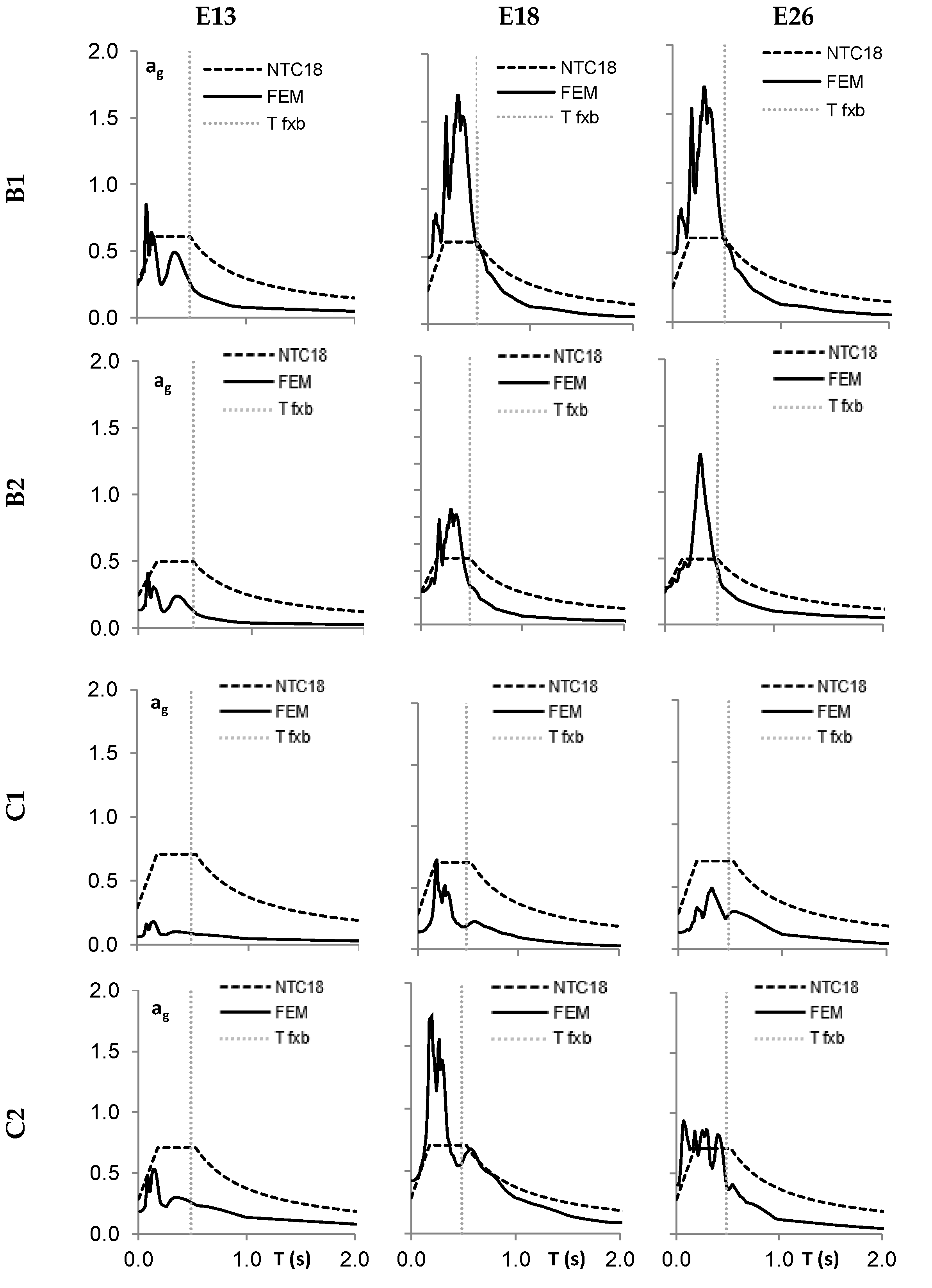
24], i.e., degrading the soil shear modulus and damping ratio according to the expected PHA at the ground surface; the second group of analyses were conducted in the nonlinear field, by means of a visco-elasto-plastic constitutive model, characterized by isotropic and kinematic hardening and a non-associated flow rule. The three inputs used, labeled E13, E18, and E26, were scaled to two accelerations: 0.10 g and 0.30 g.
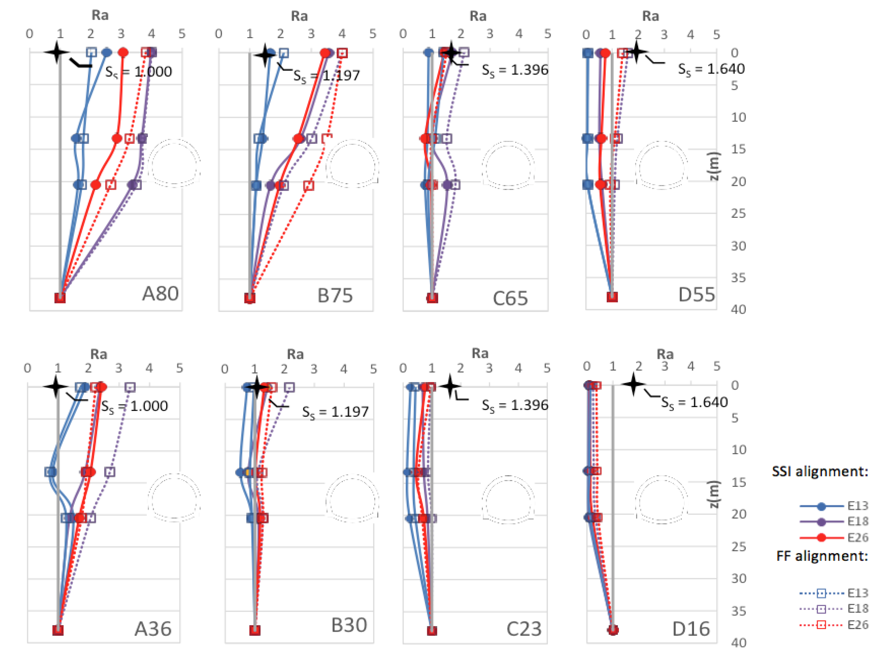
The results have been presented in terms of: acceleration amplification ratios, amplification functions, response spectra, and bending moments in the tunnels. A free-field alignment (FF) and an alignment crossing the tunnel and the aboveground structure (SS) were considered.
Initially, the results have been compared referring to the same constitutive model and varying the average Vs value and the seismic input. Finally, the results of the soil equivalent visco-linear elastic model were compared with those of the visco-elasto-plastic constitutive model.
As for the first comparison, relating to the different Vs of the analyzed soils, it was possible to observe that, first of all, the tunnel generally caused demagnification phenomena. Furthermore, the acceleration amplification ratios showed lower values in the cases of input accelerograms scaled to 0.3 g, mainly due to the required use of a high damping ratio (10%). Comparing the different soil types subjected to the same seismic input, it can be deduced that passing from soils with higher VS values to soils with lower VS values, a minor amplification of the signal occurred, contrary to what is foreseen by the Technical Codes. This behavior was due to a higher effect of the soil damping ratio and highlights the importance of a careful estimation of soil parameters and of specific local seismic response studies.
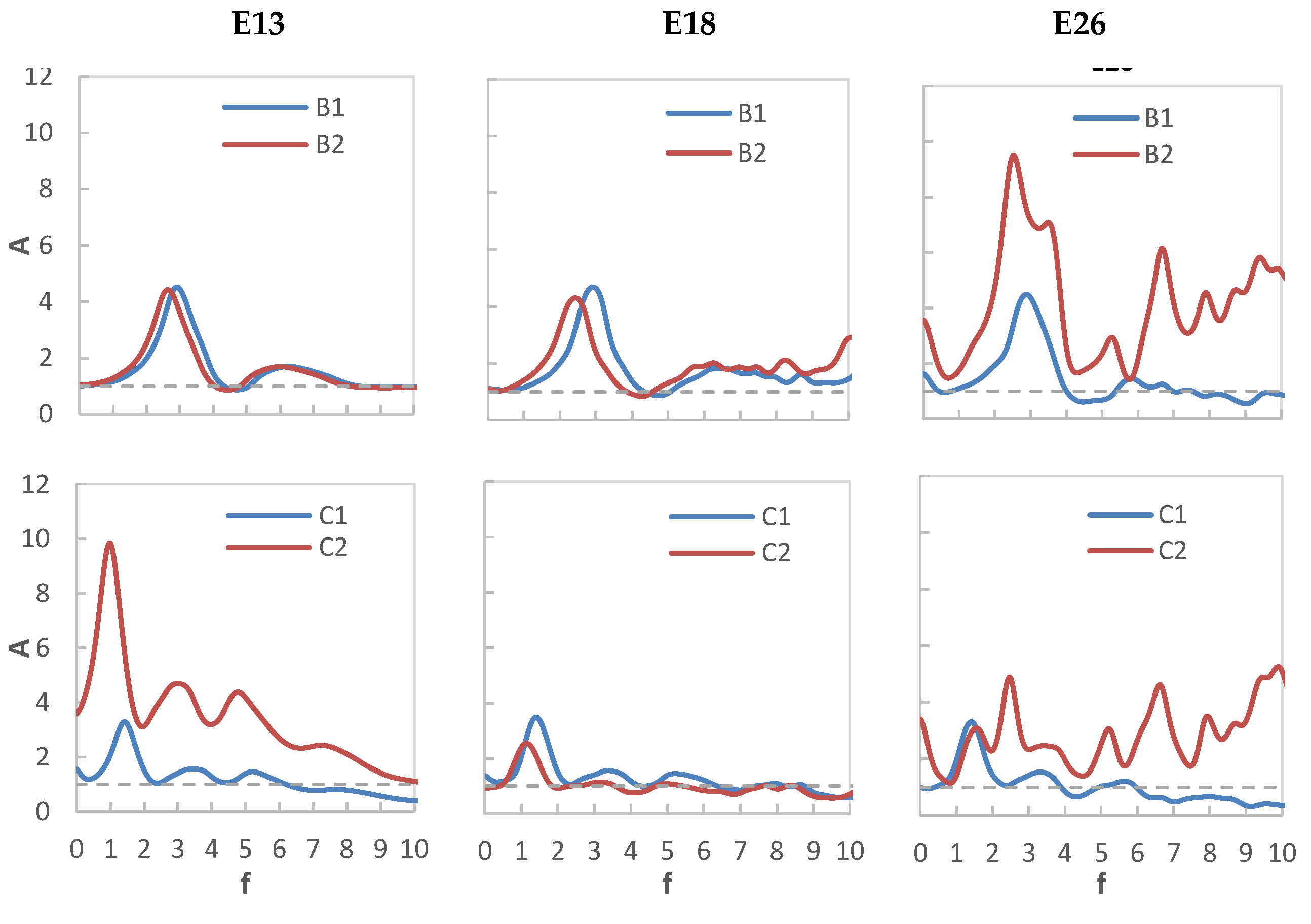
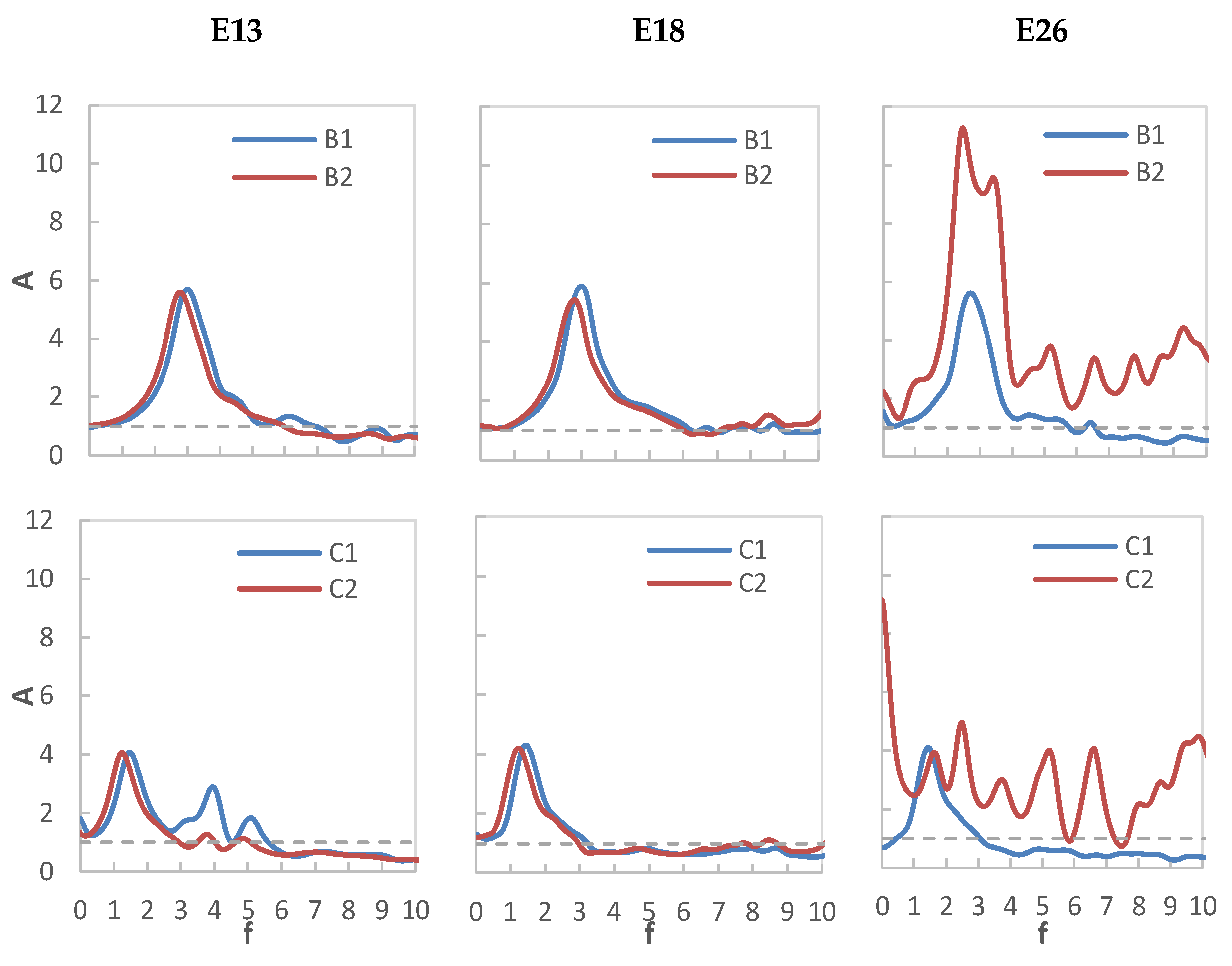
Comparing the amplification functions, the nonlinearity caused a shift of the amplification peaks towards smaller frequencies as well as an attenuation of the amplification peak.
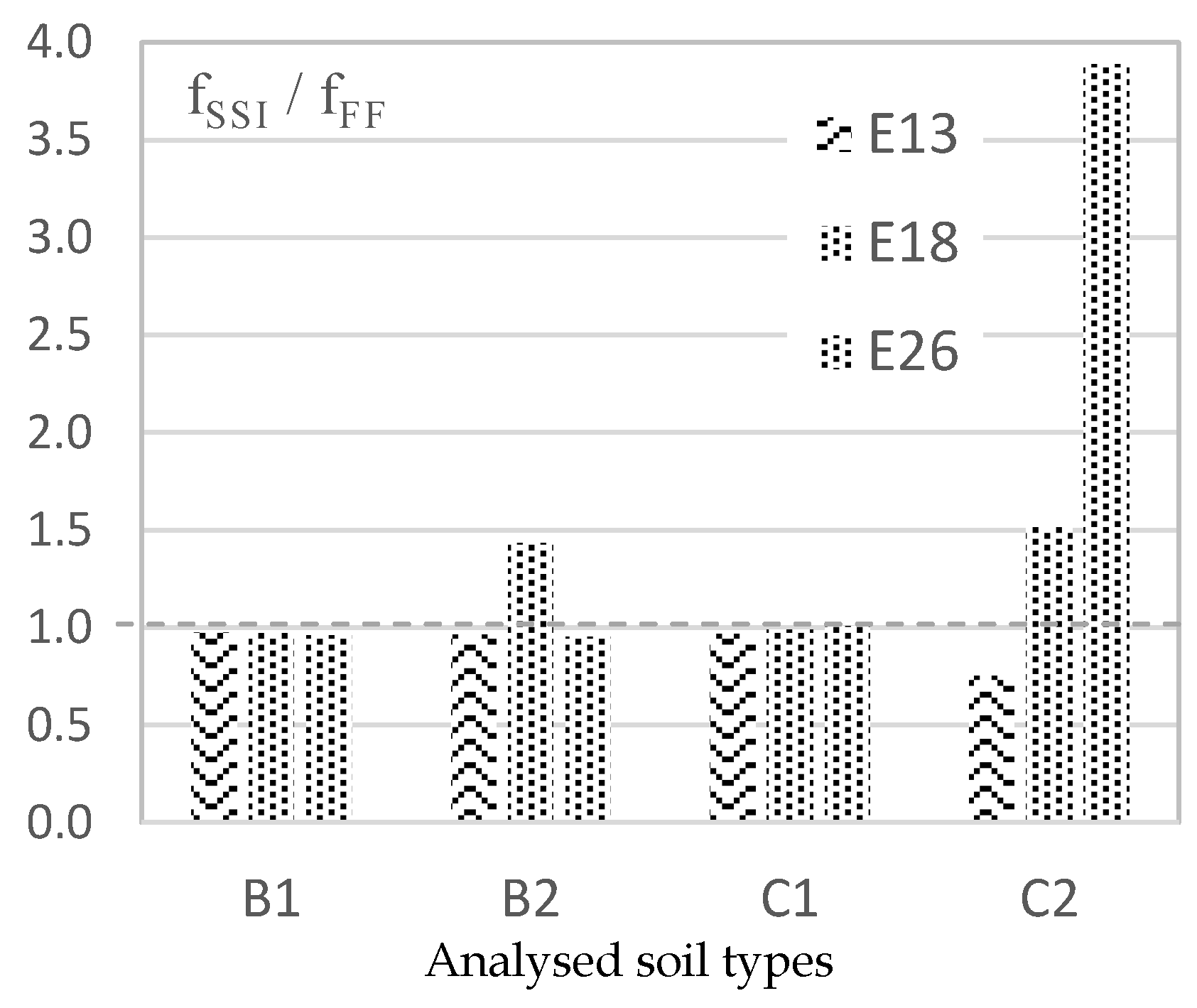
Comparing the fundamental frequencies of the inputs (finput) and of the system (fSSI, obtained with reference to the SS alignment) the probable resonance phenomena were investigated: the E13 accelerogram had a high value of the finput/fSSI ratio and therefore no resonance phenomena could occur; the E18 accelerogram showed ratios that were not particularly high but which were higher than the unit value; finally, the E26 accelerogram could cause resonance phenomena, due to the proximity of finput to fSSI. Furthermore, through the comparison between the frequencies of the two FF and SS alignments examined it is clear that the influence of the structures was minimal.
In regards to the response spectra, it can be observed that neglecting a local seismic response study and considering the spectra provided by [24] might be detrimental in some cases. In particular, for the cases under analysis, the spectrum provided by [24] tended to be safer than the FEM ones for soils characterized by lower VS values and concordant with the numerical ones or slightly detrimental for soils having higher VS values.
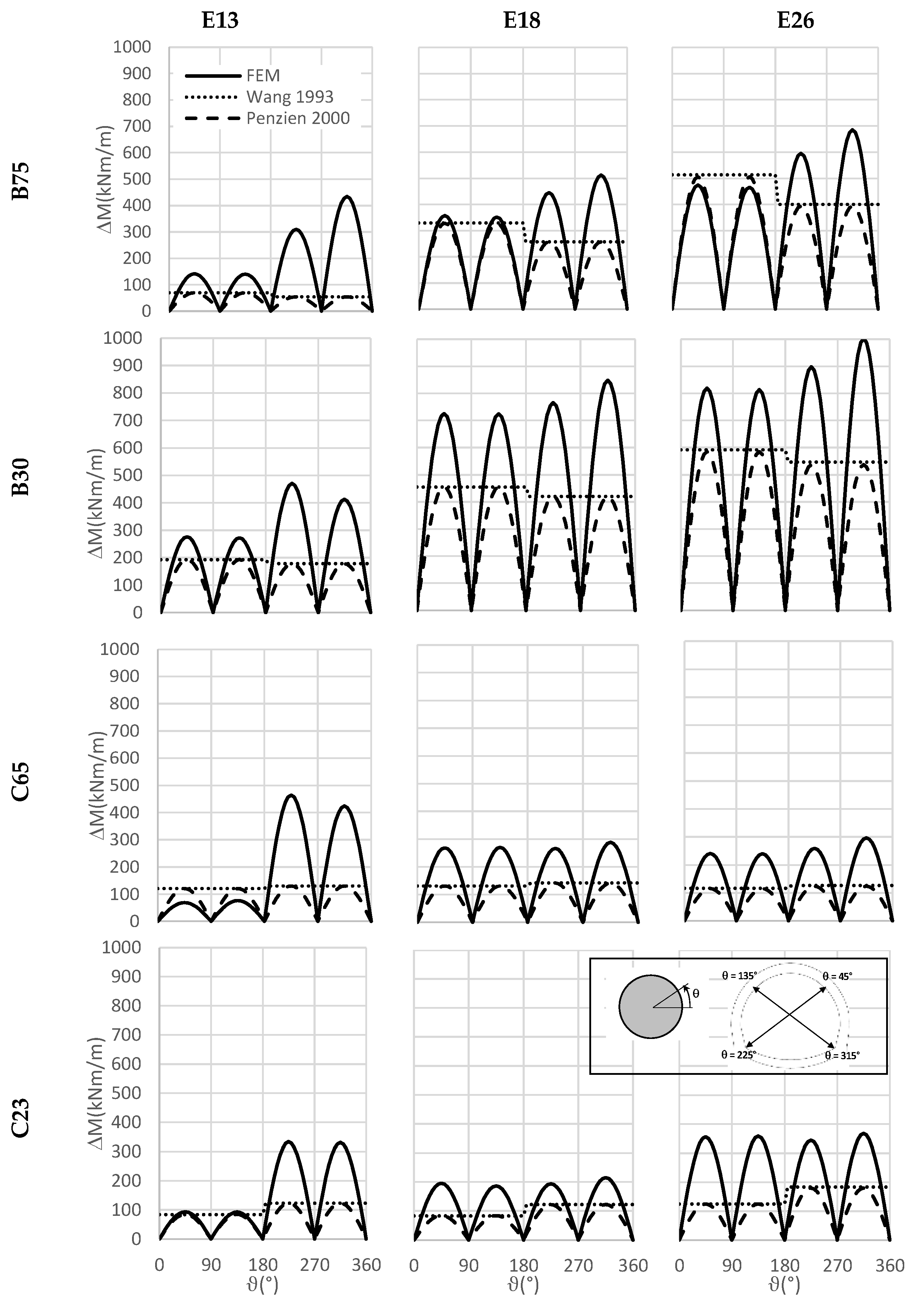
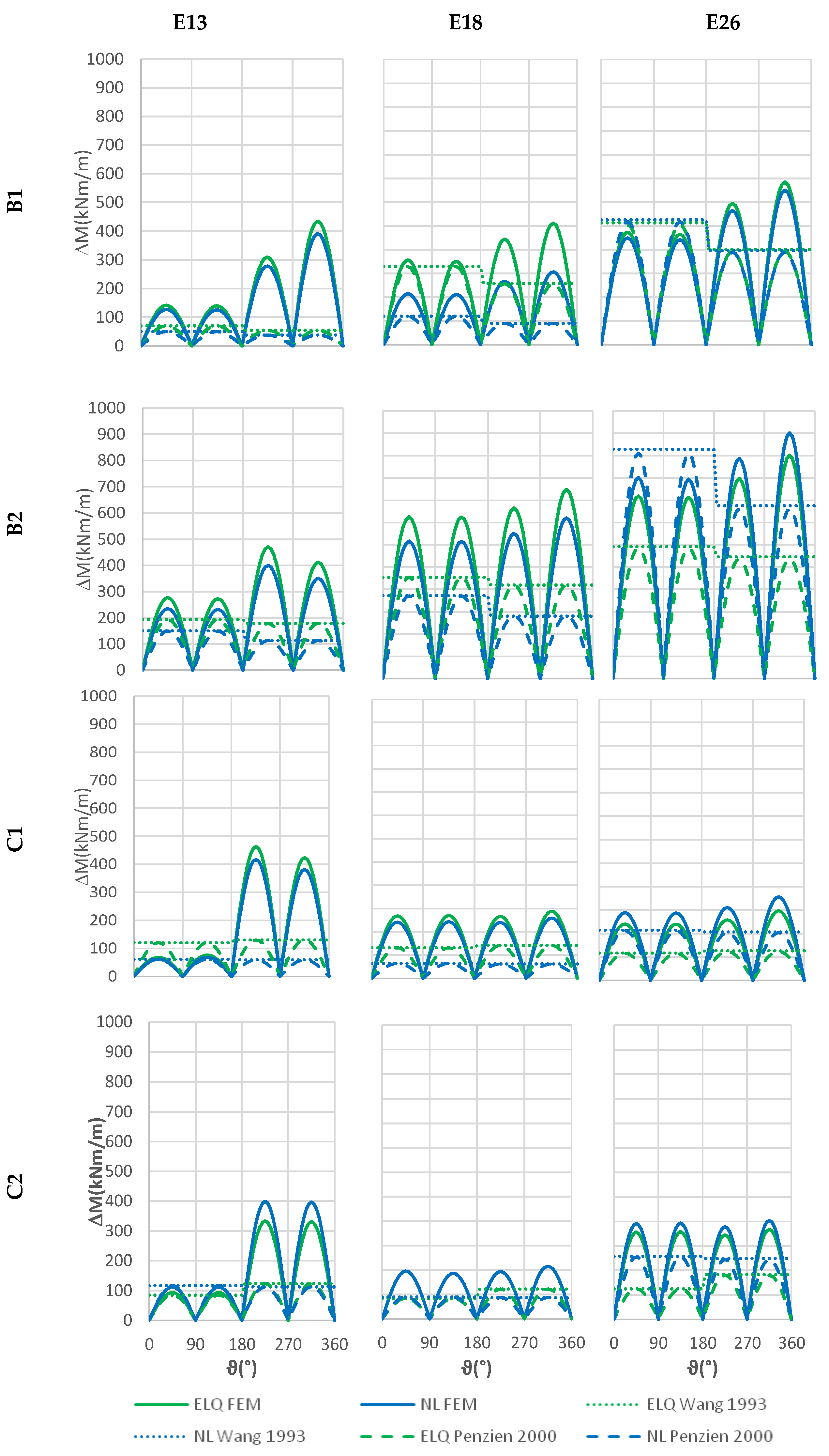
As for the bending moments in the tunnel, the comparison between the FEM and analytical [29,30] results was satisfactory in the upper arc of the tunnel, instead in the lower arc of the tunnel the analytical methods led to an underestimation of the moments compared to those derived by FEM analyses.
Regarding to the comparison between the two adopted soil models, i.e., the equivalent visco-linear elastic model and the visco-elasto-plastic constitutive one, the main results were summarized in the following.
The amplification ratio had almost the same trend in both cases. In particular, in the case of accelerograms scaled to 0.1 g, slightly higher amplification ratios were achieved by the equivalent visco-linear analyses. Instead, in the case of accelerograms scaled to 0.3 g, the maximum values of the amplification ratios were obtained by the nonlinear analysis. The differences between the two constitutive models were however minimal and this makes it possible to affirm that the same soil filter effect was achieved by both models.
Comparing the amplification functions, the fundamental frequencies obtained by the equivalent linear visco-elastic model were slightly smaller than those obtained by the nonlinear model.
As for the response spectra, the spectral ordinates obtained by the two different constitutive models were comparable to each other. In addition, the bending moments in the tunnel achieved by the two different models were comparable to each other.
It can be deduced that for relatively low accelerations the use of a nonlinear constitutive model for the soil can be avoided, because it requires a higher computational cost, but it generally leads to very similar results to those obtainable by an equivalent linear elastic modeling, carried out by simply following the EC8 suggestions. Moreover, the use of a nonlinear analysis requires the determination of many parameters; it is therefore justified only in the presence of strong seismic inputs that lead to serious nonlinear phenomena in the soil. Results of these studies could be very useful to seismic microzonation [48,49,50].

Author Contributions

G.A., S.G. and M.R.M. carried out the investigation and prepared the original manuscript according to the following percentages: 34% G.A, 33% S.G. and 33% M.R.M.

Funding

This research received no external funding.

Conflicts of Interest

The authors declare no conflict of interest.

References

  1. Kawashima, K. Seismic design of underground structures in soft ground: A review. In Geotechnical Aspects of Underground Construction in Soft Ground; Fujita, M., Ed.; Balkema: Rotterdam, The Netherlands, 2000. [Google Scholar]
  2. Hashash, Y.M.; Hook, J.J.; Schmidt, B.; Yao, J.I.-C. Seismic design and analysis of underground structures. Tunn. Undergr. Space Technol. 2001, 16, 247–293. [Google Scholar] [CrossRef]
  3. Wang, W.; Wang, T.; Su, J.; Lin, C.; Seng, C.; Huang, T. Assessment of damage in mountain tunnels due to the Taiwan Chi-Chi Earthquake. Tunn. Undergr. Space Technol. 2001, 16, 133–150. [Google Scholar] [CrossRef]
  4. Menkiti, C.O.; Kontoe, S.; Zdravkovic, L.; Potts, D.M. Case study on seismic tunnel response. Can. Geotech. J. 2008, 45, 1743–1764. [Google Scholar] [Green Version]
  5. Wang, Z.; Gao, B.; Jiang, Y.; Yuan, S. Investigation and assessment on mountain tunnels and geotechnical damage after the Wenchuan earthquake. Sci. China Ser. E Technol. Sci. 2009, 52, 546–558. [Google Scholar] [CrossRef]
  6. Gazetas, G. Case histories of tunnel failures during earthquakes and during construction. In Proceedings of the half-day conference a tunnel/underground station failure conference, by the Israeli Geotechnical Society, Herzelia, Israe, 19 January 2014. [Google Scholar]
  7. Lee, V.; Karl, J. Diffraction of SV waves by underground, circular, cylindrical cavities. Soil Dyn. Earthq. Eng. 1992, 11, 445–456. [Google Scholar] [CrossRef]
  8. Luco, J.; De Barros, F. Diffraction of obliquely incident waves by a cylindrical cavity embedded in a layered viscoelastic half-space. Soil Dyn. Earthq. Eng. 1993, 12, 159–171. [Google Scholar]
  9. Hashash, Y.M.; Park, D.; Yao, J.I.-C. Ovaling deformations of circular tunnels under seismic loading, an update on seismic design and analysis of underground structures. Tunn. Undergr. Space Technol. 2005, 20, 435–441. [Google Scholar] [CrossRef]
  10. Anastasopoulos, I.; Gerolymos, N.; Drosos, V.; Kourkoulis, R.; Georgarakos, T.; Gazetas, G. Nonlinear Response of Deep Immersed Tunnel to Strong Seismic Shaking. J. Geotech. Geoenvironmental Eng. 2007, 133, 1067–1090. [Google Scholar] [CrossRef]
  11. Anastasopoulos, I.; Gerolymos, N.; Drosos, V.; Georgarakos, T.; Kourkoulis, R.; Gazetas, G. Behaviour of deep immersed tunnel under combined normal fault rupture deformation and subsequent seismic shaking. Bull. Earthq. Eng. 2008, 6, 213–239. [Google Scholar] [CrossRef]
  12. Anastasopoulos, I.; Gazetas, G. Analysis of cut-and-cover tunnels against large tectonic deformation. Bull. Earthq. Eng. 2010, 8, 283–307. [Google Scholar] [CrossRef]
  13. Hung, C.J.; Monsees, J.; Munfah, N.; Wisniewski, J. Technical manual for design and construction of road tunnels—Civil elements; Parsons Brinckerhoff, Inc.: New York, NY, USA, December 2009. [Google Scholar]
  14. Lanzano, G.; Bilotta, E.; Russo, G.; Silvestri, F.; Madabhushi, S.P.G.; Madabhushi, S.P.G. Centrifuge Modeling of Seismic Loading on Tunnels in Sand. Geotech. Test. J. 2012, 35, 104348. [Google Scholar] [CrossRef]
  15. Abate, G.; Massimino, M.R.; Maugeri, M. Numerical modelling of centrifuge tests on tunnel-soil systems. Bull. Earthq. Eng. 2015, 13, 1927–1951. [Google Scholar] [CrossRef]
  16. Luco, J.E.; De Barros, F.C.P. Dynamic displacements and stresses in the vicinity of a cylindrical cavity embedded in a half-space. Earthq. Eng. Struct. Dyn. 1994, 23, 321–340. [Google Scholar] [CrossRef]
  17. Kouretzis, G.; Bouckovalas, G.; Sofianos, A.; YioutaMitra, P. Detrimental effects of urban tunnels on design seismic ground motions. In Proceedings of the 2nd Japan-Greece Workshop on Seismic Design, Observation, and Retrofit of Foundations, Tokyo, Japan, 3–4 April 2007. [Google Scholar]
  18. Smerzini, C.; Avilés, J.; Paolucci, R.; Sánchez-Sesma, F.J. Effect of underground cavities on surface earthquake ground motion under SH wave propagation. Earthq. Eng. Struct. Dyn. 2009, 38, 1441–1460. [Google Scholar] [CrossRef]
  19. Wang, H.-F.; Lou, M.-L.; Chen, X.; Zhai, Y.-M. Structure–soil–structure interaction between underground structure and ground structure. Soil Dyn. Earthq. Eng. 2013, 54, 31–38. [Google Scholar] [CrossRef]
  20. Abate, G.; Corsico, S.; Massimino, M.R. FEM modeling of the seismic behavior of a tunnel-soil-aboveground building system: A case history in Catania (Italy). Procedia Eng. 2016, 158, 380–385. [Google Scholar] [CrossRef]
  21. Caruso, S.; Ferraro, A.; Grasso, S.; Massimino, M.R. Site response analysis in eastern sicily based on direct and indirect Vs measurements. In Proceedings of the 1st IMEKO TC4 international workshop on metrology for geotechnics, metrogeotechnics 2016, Benevento, Italy, 17–18 March 2016; pp. 115–120. [Google Scholar]
  22. Ferraro, A.; Grasso, S.; Massimino, M.R.; Maugeri, M. Influence of geotechnical parameters and numerical modelling on local seismic response analysis. In Proceedings of the 16th European conference on soil mechanics and geotechnical engineering, ECSMGE 2015, Edinburgh International Conference Center, Edinburgh, UK, 13–17 September 2015; Volume 4, pp. 2183–2188. [Google Scholar]
  23. Castelli, F.; Cavallaro, A.; Ferraro, A.; Grasso, S.; Lentini, V.; Massimino, M.R. Static and dynamic properties of soils in Catania (Italy). Ann. Geophys-Italy 2018, 61. [Google Scholar] [CrossRef]
  24. NTC - D.M. 17/01/18 - Update technical standards for buildings, Official Journal of the Italian Republic, 17th January 2018 (in Italian). Available online: https://www.gazzettaufficiale.it/eli/gu/2018/02/20/42/so/8/sg/pdf (accessed on 27 September 2019).
  25. Pitilakis, K.; Tsinidis, G.; Leanza, A.; Maugeri, M. Seismic behaviour of circular tunnels accounting for above ground structures interaction effects. Soil Dyn. Earthq. Eng. 2014, 67, 1–15. [Google Scholar] [CrossRef]
  26. EC8 - Design of structures for earthquake resistance. European Pre-standard. ENV 1998. Europ. Com. for Standard. Bruxelles. 2003. Available online: https://www.phd.eng.br/wp-content/uploads/2015/02/en.1998.1.2004.pdf (accessed on 27 September 2019).
  27. Gajo, A.; Wood, D.M. A kinematic hardening constitutive model for sands: The multiaxial formulation. Int. J. Numer. Anal. Methods Geomech. 1999, 23, 925–965. [Google Scholar] [CrossRef]
  28. Abate, G.; Caruso, C.; Massimino, M.R.; Maugeri, M. Validation of a New Soil Constitutive Model for Cyclic Loading by FEM Analysis. Contact Mech. 2007, 146, 759–768. [Google Scholar]
  29. Wang, J.N. Seismic Design of Tunnels: A Simple State of the Art Design Approach; Parsons Brinckerhoff Inc.: New York, NY, USA, 1993. [Google Scholar]
  30. Penzien, J. Seismically induced racking of tunnel linings. Earthq. Eng. Struct. Dyn. 2000, 29, 683–691. [Google Scholar] [CrossRef]
  31. Bathe, K.J. Finite Element Procedures; Prentice Hall: New Jersey, NJ, USA, 1996. [Google Scholar]
  32. ADINA. Automatic dynamic incremental nonlinear analysis. In Theory and Modelling Guide; ADINA R&D: Watertown, MA, USA, 2008. [Google Scholar]
  33. Grassi, F.; Massimino, M.R. Evaluation of kinematic bending moments in a pile foundation using the finite element approach. WIT Trans. Built Environ. 2009, 104, 479–488. [Google Scholar]
  34. Abate, G.; Massimino, M.R. Dynamic soil-structure interaction analysis by experimental and numerical modelling. Riv. Ital. Geotec. 2016, 50, 44–70. [Google Scholar]
  35. Abate, G.; Massimino, M.R.; Romano, S. Finite Element analysis of DSSI effects for a building of strategic importance in Catania (Italy). Procedia Eng. 2016, 158, 374–379. [Google Scholar] [CrossRef]
  36. Maugeri, M.; Abate, G.; Massimino, M.R. Soil-Structure interaction for seismic improvement of noto Cathedral (Italy). Geotech. Geol. Eng. 2012, 16, 217–239. [Google Scholar]
  37. Massimino, M.R.; Abate, G.; Corsico, S.; Louarn, R. Comparison between two approaches for non-linear FEM modelling of the seismic behaviour of a coupled soil–structure system. Geotech. Geol. Eng. 2019, 37, 1957–1975. [Google Scholar] [CrossRef]
  38. Gajo, A.; Muir Wood, D. Numerical Analysis of Behaviour of Shear Stacks under Dynamic Loading; Report of ECOEST Project, EERC laboratory; Bristol University: Bristol, UK, 1997. [Google Scholar]
  39. Abate, G.; Massimino, M.R.; Maugeri, M. Finite element modeling of a shaking table test to evaluate the dynamic behaviour of a soil-foundation system. In Proceedings of the AIP Conference, Reggio Calabria, Italy, 8–11 July 2008; Volume 1020, pp. 569–576. [Google Scholar]
  40. Abate, G.; Massimino, M.R.; Maugeri, M.; Muir Wood, D. Numerical modelling of a shaking table test for soil-foundation-superstructure interaction by means of a soil constitutive model implemented in a FEM code. Geotech. Geol. Eng. 2010, 28, 37–59. [Google Scholar] [CrossRef]
  41. Lanzo, G.; Silvestri, F. Risposta Sismica Locale: Teorie ed Esperienze; Helvius: Napoli, Italy, 1999. [Google Scholar]
  42. Bonaccorso, R.; Grasso, S.; Giudice, E.L. Cavities and hypogeal structures of the historical part of the City of Catania. WIT Trans. State-of-the-art Sci. Eng. 2005, 1, 197–223. [Google Scholar]
  43. Cavallaro, A.; Grasso, S.; Maugeri, M. Volcanic soil characterisation and site response analysis in the city of Catania. In Proceedings of the 8th national conference on earthquake engineering, San Francisco, CA, USA, , 18–22 April 2006; pp. 835–844. [Google Scholar]
  44. Cavallaro, A.; Ferraro, A.; Grasso, S.; Maugeri, M.; Santini, A.; Moraci, N. Site Response Analysis of the Monte Po Hill in the City of Catania. AIP Conf. Pro. 2008, 1020, 240–251. [Google Scholar]
  45. Cavallaro, A.; Ferraro, A.; Grasso, S.; Maugeri, M. Topographic Effects of the Monte Po Hill in Catania. Soil Dyn. Earthq. Eng. 2012, 43, 97–113. [Google Scholar] [CrossRef]
  46. NTC - D.M. 14/01/08 - New technical standards for buildings, Official Journal of the Italian Republic, 14th January 2008 (in Italian). Available online: https://www.gazzettaufficiale.it/eli/id/2008/02/04/08A00368/sg (accessed on 27 September 2019).
  47. Idriss, I.M.; Seed, H.B. Seismic response of horizontal soil layers. Soil Mech Found Eng ASCE 1968, 94, 1003–1031. [Google Scholar]
  48. Grasso, S.; Maugeri, M. Seismic microzonation studies for the city of Ragusa (Italy). Soil Dyn. Earthq. Eng. 2014, 56, 86–97. [Google Scholar] [CrossRef]
  49. Ferraro, A.; Grasso, S.; Maugeri, M.; Totani, F. Seismic response analysis in the southern part of the historic centre of the City of L’Aquila (Italy). Soil Dyn. Earthq. Eng. 2016, 88, 256–264. [Google Scholar] [CrossRef]
  50. Castelli, F.; Cavallaro, A.; Grasso, S.; Lentini, V. Seismic microzoning from synthetic ground motion earthquake scenarios parameters: The case study of the city of Catania (Italy). Soil Dyn. Earthq. Eng. 2016, 88, 307–327. [Google Scholar] [CrossRef]
Figure 1. The real cross-section referring to a segment of the underground railway in Catania (Italy).
Geosciences 09 00473 g001
Figure 2. FEM model adopted.
Geosciences 09 00473 g002
Figure 3. Comparison between amplification ratios in the symmetry axis of the building and of the tunnel (SS) and free-field conditions (FF) alignments for the eight models studied in the equivalent visco-linear elastic analyses.
Geosciences 09 00473 g003
Figure 4. Comparison among amplification ratio profiles achieved for different configurations of the analyzed system (after [20]).
Geosciences 09 00473 g004
Figure 5. Flexibility ratios for the eight models studied in the equivalent visco-linear elastic analyses.
Geosciences 09 00473 g005
Figure 6. Comparison between numerical and analytical bending moments for some models (soil types B and C) studied in the equivalent visco-linear elastic analyses.
Geosciences 09 00473 g006
Figure 7. Comparison between the amplification functions obtained for the SS alignment.
Geosciences 09 00473 g007
Figure 8. Comparison between the amplification functions obtained for the FF alignment.
Geosciences 09 00473 g008
Figure 9. Comparison between the input frequencies finput and the soil frequencies fSSI (evaluated considering the SS alignment).
Geosciences 09 00473 g009
Figure 10. Comparison between the SSI (Soil-Structure Interaction) and the FF frequencies.
Geosciences 09 00473 g010
Figure 11. Comparison between response spectra at the base of the structure achieved by numerical analyses and provided by [24].
Geosciences 09 00473 g011
Figure 12. Comparison between amplification ratios in SSI and FF alignments for the eight models studied in the visco-nonlinear analyses.
Geosciences 09 00473 g012
Figure 13. Comparison between numerical and analytical bending moments for the models B1, B2, C1, and C2.
Geosciences 09 00473 g013
Figure 14. Comparison between the amplification functions obtained for the SS alignment (visco-nonlinear analyses).
Geosciences 09 00473 g014
Figure 15. Comparison between the amplification functions obtained for the FF alignment (visco-nonlinear analyses).
Geosciences 09 00473 g015
Figure 16. Comparison between the input frequencies finput and the soil frequencies fSSI for the SS alignment (visco-nonlinear analyses).
Geosciences 09 00473 g016
Figure 17. Comparison between the SS and the FF frequencies (visco-nonlinear analyses).
Geosciences 09 00473 g017
Figure 18. Comparison between response spectra at the base of the structure achieved by numerical analyses and provided by [24] (visco-nonlinear analyses).
Geosciences 09 00473 g018
Figure 19. Comparison between amplification ratios in SSI alignment for the two different constitutive models (equivalent visco-linear elastic—ELQ vs. nonlinear—NL).
Geosciences 09 00473 g019
Figure 20. Comparison between the amplification functions in the SS alignment for the two different constitutive models (ELQ vs. NL).
Geosciences 09 00473 g020
Figure 21. Comparison between response spectra at the base of the structure obtained by the two different constitutive models (ELQ vs. NL) and provided by [24].
Geosciences 09 00473 g021
Figure 22. Comparison between analytical and numerical bending moments obtained by the two different constitutive models (ELQ vs. NL).
Geosciences 09 00473 g022
Table 1. The different shear wave velocity VS adopted for the different soil types analyzed and the corresponding stratigraphic amplification factor SS provided by [24].
Soil typesVs (m/s)Vs * (m/s)Ss
A>80010001.000
B360 ÷ 8005001.197
C180 ÷ 3602501.396
D<1801001.640
VS * indicates the chosen values; VS indicates the ranges provided by [24].
Table 2. The input motions adopted.
InputsOriginal ag (m/s2)f1 (Hz)f2 (Hz)f3 (Hz)Time History
E13 (Timfristos, Greece 1986)3.0212.706.868.26 Geosciences 09 00473 i001
E18 (Friuli, Italy 1976)1.595.534.544.24 Geosciences 09 00473 i002
E26 (Friuli, Italy 1976)1.832.953.262.12 Geosciences 09 00473 i003
Table 3. Values of damping ratio (D) and degradation of VS and shear modulus (G; after [26]).
Expected Surface Acceleration, SS∙agDVs/Vs,maxG/Gmax
0.100.030.9 ± 0.070.80 ± 0.10
0.200.060.7 ± 0.150.50 ± 0.20
0.300.100.6 ± 0.15 0.36 ± 0.20
Table 4. Parameters adopted for the eight models developed in equivalent linear visco-elastic analyses.
ModelSS∙ag (g)G/GmaxDoperativeGoperative (MPa)
A800.100.800.031600
B750.120.750.03375
C650.140.650.0381.25
D550.160.550.0311
A360.300.360.10720
B300.360.300.10150
C230.420.230.1028.75
D160.490.160.103.2
Table 5. Parameters adopted for the four models developed for the non-linear analyses
Soil ParameterSoil Type B:Soil Type C:
B1 (ag = 0.1 g)B2 (ag = 0.3 g)C1 (ag = 0.1 g)C2 (ag = 0.3 g)
E (MPa)1300325
ν0.30.3
φcv (°)2424
λ0.060.06
vλ1.7121.712
R0.010.01
A0.90.9
kd11
B0.010.01
k22
D0.030.100.030.10
Table 6. Comparison between the soil fundamental frequencies for the two models (ELQ and NL).
B1B2C1C2
fSSI,ELQ (Hz)fSSI,NL (Hz)fSSI,ELQ/fSSI,NLfSSI,ELQ (Hz)fSSI,NL (Hz)fSSI,ELQ/fSSI,NLfSSI,ELQ (Hz)fSSI,NL (Hz)fSSI,ELQ/fSSI,NLfSSI,ELQ (Hz)fSSI,NL (Hz)fSSI,ELQ/fSSI,NL
E132.542.970.861.582.740.584.301.462.950.650.970.67
E182.562.980.862.082.410.861.101.440.760.731.150.63
E262.562.900.881.222.530.481.151.460.791.972.100.94

