Abstract
Forecasting estuarine circulation is a hot topic, especially in densely populated regions, like Santos (Brazil). This paper aims to improve a water-level forecasting system for the Santos estuary, particularly the physical forcing determining the residual tide, which in extreme cases increase the predicting errors. The MOHID hydrodynamic model was implemented with a nested downscaling approach. All automatic procedures to provide a high-resolution real-time forecast system are managed by the AQUASAFE software. Water-level observation and prediction datasets (2016–2017) of five tide gauges in the Santos channel were analyzed, resulting in distinct model configurations, aiming to minimize forecasting inaccuracies. Current MOHID open boundary reference solutions were modified: the astronomical solution was updated from FES2012 to FES2014 whereas the meteorological component (Copernicus Marine Environment Monitoring Service (CMEMS) global solution) time resolution was altered from daily to hourly data. Furthermore, the correlation between significant wave height with positive residual tide events was identified. The model validation presented a minimum Root Mean Square Error (RMSE) of 12.5 cm. Despite FES2014 solution improvements at the bay entrance, errors increase in inner stations were maintained, portraying the need for better bathymetric data. The use of a CMEMS hourly resolution decreased the meteorological tide errors. A linear regression method was developed to correct the residual tide through post-processing, under specific wave height conditions. Overall, the newest implementation increased the water-level forecast accuracy, particularly under extreme events.
1. Introduction
From a human historical perspective, the intrinsic characteristics of estuaries have made them preferable sites of occupation and, consequently, intense areas of development. The Santos estuary (Brazil) is a very important estuarine system, in which the main socio-economic drivers are industrial and port activities. Moreover, the Port of Santos, the most important harbor in Latin America, plays a significant role in the Brazilian and international economy [1]. Cubatão city (north of the Santos estuary) has a relevant industrial complex, mainly associated with petroleum products, fertilizer production and important steel production [1]. Therefore, the Santos estuary not only endures great urban pressure regarding the large population that live near its margins but also from the activities employed in this area. Consequently, there is a significant interest in understanding the physical processes driving the estuary’s circulation in order to support effective decision-making regarding specific coastal activities. Monitoring water level and wave data comprehend different applications, such as control of the national leveling system, oceanographic studies, climate change impacts assessment, operational purposes, harbor operations, navigation, etc. Furthermore, several factors contribute to coastal ocean model forecast uncertainties, including imperfect atmospheric forcing fields; boundary condition errors propagating inside the finer-scale model domain; bathymetric errors; insufficient horizontal and vertical resolution; numerical noise; bias; errors in parameterizations of atmosphere–ocean interactions and sub-grid turbulence, etc. [2]. It is essential to highlight the absolute importance of local- and coastal-scale operational oceanography to support the decision-making as well as scientific research. Currently, HIDROMOD (https://hidromod.com/home-pt/) together with UNISANTA (Universidade Santa Cecília) is responsible for a forecast system management—AQUASAFE (waves, water level, currents, water quality [3]), used to support real-time harbor, civil protection, and water-quality monitoring activities for the Santos Estuary. The AQUASAFE platform (www.aquasafeonline.net), was developed by HIDROMOD (Lisbon, Portugal), and distinguished by International Water Association (IWA). The water level and wave climate variability in the Santos estuary, under extreme conditions, prevents a wide range of uses, such as commercial and recreational navigation. In addition, drainage and urban floods affect the local beach water quality. Over time, particularly in the Santos system, an effort has been made in attempting to decrease prediction errors, mainly in the water level forecast service provided by AQUASAFE. Thereafter, several improvements were achieved, where continuous data validation allows the permanent improvement of this forecasting system, in line with scientific advances. The ensemble factors affecting the estuary hydrodynamics (tides, meteorology, freshwater discharges) continue to present a challenging task in improving the forecast capacity of the models. More precisely, the Santos complex water-level regime engenders great difficulties for local tide prediction. In extreme cases, e.g., storm surges, predicted and observed water levels can significantly differ in height, strongly increasing the tide prediction errors and restricting the forecasting model’s accuracy. This limitation adversely affects the programming of shipping procedures and navigation, as well as timely warnings of urban floods to populations. The latter occur under intense precipitation events with high water levels.
The above highlights the motivation and need to fully address the main physical factors influencing the Santos estuary hydrodynamics. Hence, this work aims to analyze historical water-level datasets, investigate in which conditions (atmospheric and oceanographic) the present forecast system results have major limitations, and further investigate hypotheses to decrease these errors. Bearing in mind the continuous challenge in improving forecast services, boundary conditions data sources were upgraded, attempting to decrease forecasting errors whilst improving the operational system for extreme tidal events.
Study Area
The Santos estuary (Figure 1) is located in the South-East Brazilian coastal area (23°30′–24° S; 46°05′–46°30′ W), comprising an 835 km2 basin area [4]. The estuarine system of Santos consists of three major channels, namely S. Vicente, Santos, and Bertioga, interconnected in the inner area. The Santos and S.Vicente channels cover an approximate area of 44.100 m2, with an average depth of 15 m in the central dredged channel of Santos and 8 m in S.Vicente channel [1].
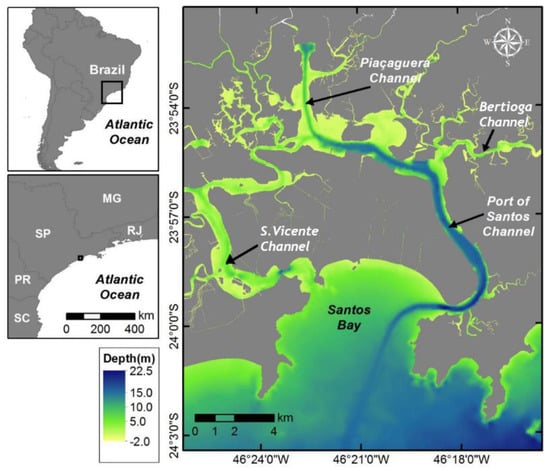
Figure 1.
Map of the study area with the location of the Port of Santos. Adapted from: [5].
The estuarine system is characterized by a flat area surrounded by scarps of the plateau of Serra do Mar [1], and bordered by the cities of Santos, S. Vicente, Guarujá, Bertioga and Cubatão, which is one the most industrialized areas of South America [6]. The Santos estuary can be classified as a typical sub-tropical mangrove system, under significant anthropogenic pressure. Santos harbor is the most important port in Brazil and the largest harbor in Latin America, which traded more than 110 million tons of cargo in the year 2018 [7]. The Santos estuary is a complex system whose geometry and river discharge has been drastically altered during the last century by urban and industrial development, land reclamation, dredging and effluent reception from multiple industries [6]. The estuary receives freshwater inflow from several small rivers that develop on the slopes of Serra do Mar, at heights of 700 meters [8]. Therefore, six main rivers discharge into the Santos estuary, namely a discharge of rivers Cubatão’s effluent (major freshwater contributor), the rivers Moji and Piaçaguera discharging together, and rivers Quilombo, Jurubatuba, and Borturoca, with approximately 10 m3/s average flow. The main forcing agent driving water circulation is the tide, with an average amplitude of 1.43 m (measured at Santos port), being considered a micro-tidal estuary. The estuary is partially mixed to stratified, where the salt transport within the estuary is due to the up-estuary propagation of the salt wedge and eddy diffusion [6], inducing changes in circulation patterns.
The South-East Brazilian shelf is known for the resonance of the third-diurnal principal lunar tidal constituents M3 (period of 8.28 h), related to tidal current asymmetries. This constituent amplification was first described by [9], the largest amplitudes being found in the Paranaguá estuarine system [10]. Distortions are found in every two tidal cycles, indicating this component relates to the daily inequalities in the tidal amplitudes [11].
Apart from the astronomical tide, the meteorological tide provides significant changes in the water levels of this region. An annual average of 12 positive extreme events of water level were counted in the analysis of [12], associated with south-westerly wind velocities above 8 m/s over the ocean, along with a continental anticyclone presence. These highly energetic events in the estuary of Santos are related to coastal erosion and flooding in adjacent areas [11,12,13]. Cold fronts (often during winter) influence water level fluctuations that may exceed 0.5 m [14,15].
According to [4,16], continental shelf waves can be one of the mechanisms behind the sub-inertial water level oscillations, observed along the South-East Brazilian coast. These waves are generated near the coast of Argentina, and due to atmospheric disturbances propagate north-east, along the South-East-Brazilian shelf.
Current velocities in the inner estuary are mostly driven by tidal forcing, reaching up to 0.5 m/s and do not present significant differences between the winter and summer periods [17].
2. Materials and Methods
2.1. Hydrodynamic Model
The hydrodynamic model used in this study was MOHID (www.mohid.com), which was developed in the IST (Instituto Superior Técnico) of the University of Lisbon (Portugal). MOHID is a hydrodynamic model designed for coastal and estuarine shallow water applications, like the study of Santos estuary dynamics.
The AQUASAFE platform was used to extract oceanographic databases used in the present work. AQUASAFE is a software platform supported by modeling tools and advanced data analysis, based on a client-server architecture and developed with a modular philosophy. It can integrate real-time data captured by sensors (local and remote) and run several models periodically to produce automatic reports for custom data analysis and comparisons between model predictions and measured data [3].
2.1.1. Governing Equations
MOHID solves the three-dimensional incompressible primitive equations assuming hydrostatic equilibrium and the Boussinesq and Reynolds approximations. The primitive equations are solved in Cartesian coordinates for incompressible flows [18,19,20], being the momentum and continuity equations represented by Equations (1) and (2), respectively:
where ui is the horizontal velocity vector (i = 1,2 directions) and uj the 3D velocity vector (j = 1,2,3), the water level, v the turbulent viscosity, patm the atmospheric pressure, ρ is the density, ρ0 is the reference density, ρ(η) represents the density at the free surface, g is the gravity acceleration, t is the time, Ω is the earth velocity of rotation and ε is the alternate tensor.
2.1.2. Model Domains
The numerical grid used for the Santos estuary includes a downscaling approach with four nested levels (L1, L2, L3 and L4), with different horizontal resolutions (Figure 2).
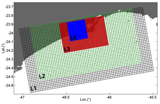
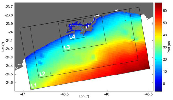
Figure 2.
Hydrodynamic numerical grids (top) and bathymetry (bottom) with 4 levels (L1, L2, L3, L4); the color scale represents the depth in meters. Adapted from [5].
A one-way nesting is undertaken. The first numerical grid (L1) is a 2D barotropic model, as are the three subsequent grids (L2, L3 e L4), using only one sigma layer in the vertical dimension. The L1 water-level ocean boundary reference solution results from adding the astronomical tide to the inverse barometer approximation. The astronomic tide is calculated from the harmonics interpolated to the open boundary cells (e.g., global tide solution FES2012) and the inverse barometer interpolating the atmospheric pressure forecasts. In L1 domain, a clamped open boundary condition for the water level is used. In all nested domains is used a hybrid open boundary condition, where a radiative boundary condition is complemented by a flow relaxation boundary condition [21]. In L2, the open boundary reference solution results from adding in run time L1 solution, and low-frequency barotropic solution coming from the CMEMS (Copernicus Marine Environment Monitoring Service) model (meteorological tide). In L3 and L4, open boundary reference solutions arise from L2 and L3 solutions, respectively. At the surface boundary are imposed the wind stress and atmospheric pressure gradients at water level. Also, for the bottom boundary, an absolute rugosity of 2.5 mm was adopted. No river discharge is considered in the land boundary. Regarding the grids characteristics, L1 has a horizontal resolution of 0.02° (~2 km) and 37 × 72 points; L2 has 31 × 61 points and a resolution of 0.02° (~2 km); L3 has a resolution of 0.004° (~ 400 m) and 85 × 130 points; and the last grid (L4) has a resolution of 0.0005° (~50 m), with 432 × 416 points.
The present four-nested levels downscaling approach allows the simulation of processes with different spatial scales on the south-eastern Brazilian shelf, providing accurate boundary conditions to the Santos estuarine system, contributing to model accuracy and efficiency. The highest resolution domain, L4 (~50 m), allows a better bathymetric representation and, therefore, a more accurate description of local processes at the Santos estuary.
The bathymetry was obtained by scanning the nautical charts of DHN (Diretoria de Hidrografia e Navegação do Brasil)—1701; 1711; 23,100 and 23,200—and by recent surveys conducted by the Santos Port (SP) Pilots and NPH-UNISANTA (Núcleo Pesquisas Hidrodinâmicas—Universidade de Santa Cecília) database (Figure 2). The astronomical tide was derived from FES2012 [22], which is a tidal global solution that provides tidal heights worldwide. This solution has been developed, implemented and validated by LEGOS (Laboratoire d’Etudes en Géophysique et Océanographie Spatiales), NOVELTIS (https://www.noveltis.com/en/noveltis/) and CLS (Collecte Localisation Satellites). It consists of 32 tidal constituents, distributed on 1/16 grids (amplitude and phase). The meteorological tide was derived from the daily solution of CMEMS [23]. The GFS (Global Forecast System), available from the NOAA (National Oceanic and Atmospheric Administration), is a meteorological prediction model produced by the NCEP (National Center for Environmental Prediction). For the Santos estuary, the daily results of the GFS model are used regarding air pressure, wind speed, and direction.
For the present work, data ranging from the years 2016–2017 was extracted from AQUASAFE to model validation, through comparison between predicted and observed water level data, collected at SP Pilots stations.
2.2. Water-Level and Wave Data
Tide measurements are collected by 5 tide gauges (10 minutes sampling frequency) and wave data (including significant peak wave and period each 20 min) measured at S1 tide gauge, for 2016–2017. The locations of the 5 stations along Santos estuary and respective coordinates are depicted in Table 1 and Figure 3.

Table 1.
Tidal gauges along Santos estuary, coordinates, and measured parameters.
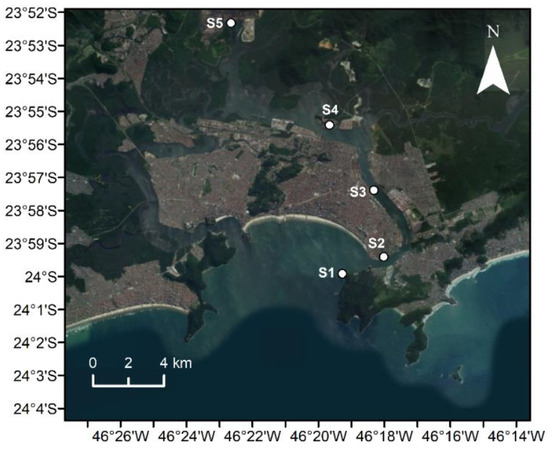
Figure 3.
Location of the 5 tide gauges (S1, S2, S3, S4 and S5) along Santos estuary.
The water-level data was used to validate the model results and to perform harmonic analysis. For this purpose, both the water level and wave databases were subject to outlier correction and filling data gaps, avoiding possible residual noise.
2.3. Statistical Analysis of Water Level
2.3.1. Astronomical Tide
Astronomical tide errors were calculated through a direct comparison between the astronomical component of predictions and observations datasets, ranging from 1 January 2016 to 1 January 2017 (10 minutes’ sampling frequency), aiming to evaluate the model forecasting capacity. These time-series were obtained using T_Tide package routines [24], to perform classical harmonic analysis of amplitude and phase of the main important solar (K1, O1, Q1, P1), lunar (M2, S2, N2, K2) and non-linear (M3, M4) constituents. Having both an amplitude (Ai) and phase lag (Gi) of each constituent, the tide height (H) can be calculated at any time (t) as the sum of contributions of each tidal constituent by the following equation:
where A0 represents the mean water level; k the number of tidal constituents; i the index of a constituent; ωi the angular velocity and (V0 + υ)i the astronomical argument. Fi and ui can be intended as the amplitude and phase corrections.
Additionally, the mean complex amplitude error (HCi) is calculated to compare the amplitude and phase of each harmonic constituent, and also the relative value of the HC (RHCi) parameter.
The h modi, h obsi, φ modi, φ obsii parameters correspond to amplitudes and phase of predictions and observations, respectively [25]. The use of HC and RHC is useful for a comprehensive view of each harmonic constant error, individually, in terms of amplitude and phase discrepancies.
2.3.2. Residual Tide
Comparing the observed water level at a tide gauge station and the predicted values obtained through harmonic synthesis, there is always a difference related to the contribution of meteorological forcing (storm surges), tide–surge interaction and errors associated with harmonic synthesis and instruments [26,27,28]. The approach applied to estimate residuals consists of subtracting the tide synthesized by harmonic analysis and total water level. Thus, the non-tidal residuals were calculated as following [28]:
where R (t) is the non-tidal residual, X (t) and (Z0 + T(t)) are the observed and synthesized level, respectively.
2.3.3. Statistical Parameters
To compare the predicted and observed data, several statistical parameters were applied. The RMSE (Root Mean Square Error) calculates the absolute measure of the model deviation from data, being one of the most used error parameters to assess tidal model performance [29,30]:
where N corresponds to the number of records and Xobs and Xmod represent observations and model predictions, respectively.
BIAS gives an indication of whether the model predictions are systematically overestimating or underestimating observations, being model predictions as better as BIAS is close to zero. It is expressed as:
Considering two-dimensional variables, Xobs and Xmod, the Correlation Coefficient (R) is expressed as:
where and represents the standard deviation of model and observations, respectively.
The predictive Skill (S) value was also computed, being a descriptive measure that reflects the degree to which the observed variable is accurately estimated by the predicted variable [31]. This index can be mathematically expressed as:
where values of 1 correspond to a perfect adjustment between predictions and observations, while values of 0 indicate a complete disagreement. Higher values than 0.95 should be considered excellent [32]. These statistics were applied to observations and predictions as well as to astronomical and residual tide components isolated for a better understanding of errors.
2.4. Optimizing Boundary Conditions
The attempt of improving model boundary conditions consisted of trying different astronomic and meteorological solutions and comparing them with the current model implementation. Therefore, the novel FES2014 astronomic solution was tested as an oceanic boundary condition for the model. Compared to FES2012, the newest version takes advantage of longer altimeter time-series, better altimeter standards, data assimilation techniques, more accurate ocean bathymetry and a refined mesh in most of the shallow water regions [33]. Hence, an improvement in non-linear constituents prediction (M3 and M4) would be expected. The CMEMS (meteorological tide), imposed in the model as an oceanic boundary condition, was tested with an hourly resolution, hypothesizing that the water level and barotropic velocity daily solution, currently in use, may not be sufficient to forecast some intense residual tide events during short time periods.
2.5. Study the Relation among Physical Variables
Additionally, it is assumed that positive residual tide forecast errors increase under extreme conditions characterized by intense variability of metocean conditions (e.g., atmospheric pressure, significant wave height, wind velocity). Consequently, the correlation between the residual tides (predictions and observations) with atmospheric parameters (wind intensity, pressure) and oceanographic parameters (significant peak wave) was evaluated, and a strong correlation could be found between residual tides and wave height. Thus, each event of Hs higher than 1.5 m during at least 3 hours, (threshold adopted for the present study), was studied for the year 2016–2017. For each event, the maximum level reached by the residual tide (predicted and observed) was found and after the error was calculated (residual predicted minus residual observed). It was found that for increasing values of Hs the residual tide error was higher. According to the results obtained, a linear regression technique was applied, the error being the dependent parameter whereas Hs the independent variable.
3. Results and Discussion
3.1. Data Analysis
The statistical analysis to evaluate model performance (comparison between predictions and observations), for a 1-year record, are presented in Table 2, including R (Correlation Coefficient), RMSE (Root Mean Square Error), UNBIAS RMSE, BIAS and S (Skill) parameters. Results for the local model (Level 4) validation are depicted for the 5 stations.
Table 2.
Statistical parameters (R (Correlation Coefficient), RMSE (Root Mean Square Error), UNBIAS RMSE, BIAS, and S (Skill)) (cm) for water level for the 5 tide gauges in Santos estuary for 2016–2017.
Regarding the predicted mean water level, no significant variability among stations was identified. On the contrary, observed mean water level presents high variability among different stations, particularly for the high BIAS presented in S2 (Table 2). The variability of the observed mean water level between stations does not have a coherent pattern suggesting a possible problem in the definition of a common vertical referential for all stations. Having this limitation, the prediction accuracy will be quantified using UNBIAS RMSE instead of RMSE. In general, results reveal a good agreement between predictions and observations (Table 2).
According to [31], a RMSE lower than 5% of the local amplitude represents an excellent agreement between model predictions and observations, while an RMSE between 5% and 10% indicates very good agreement. Along the estuary, RMSE ranges from 12.5 cm in S1 (an error of 9.6%) until 19.7 cm in S5 (an error of 15%), respectively, being the minimum UNBIAS RMSE value found in the bay entrance. S2 presents an error of 9.8%, S3 approximately 10.9% and S4 13%. Therefore, S1 and S2 stations may be considered with very good agreement. As the distance from the S1 station increases, the deviations between predictions and observations are more evident. It was suggested by [31] that water level S higher than 0.95 can be considered excellent. Bearing this in mind, an excellent agreement was found for the majority of sites S1, S2, S3, and S4. Furthermore, S values higher than 0.90 represent good agreement, in which can be included S5. R results range from 0.90 to 0.95, where higher accord is found in S1, and by contrast, lower agreement is found in S5.
3.2. Astronomical Tide Analysis
The statistical analysis to evaluate model performance in terms of the astronomical component (predictions and observations), computed for the 1-year record is depicted in Table 3, including R, UNBIAS RMSE and S parameters.
Table 3.
Statistical parameters (R, RMSE, UNBIAS RMSE, and S) (cm) for astronomical tide for the 5 tide gauges in Santos estuary for 2016-2017.
The astronomical tide UNBIAS RMSE values increase towards the inner estuary area, which may reflect at first glance the accumulative inaccuracies effect of the tide wave propagation trajectory. Secondly, this may be due to low-quality bathymetry in the inner estuary, mainly in the mangrove areas. Also, R and S parameters decrease towards the inner estuary. Although predictions and observations of RMSE can be computed to measure model performance, generally the calibration and validation procedures involve some degree of subjectivity. In fact, there is a large disadvantage in the direct comparison of RMSE errors, since phase and amplitude errors are considered together. For example, two datasets with no error in amplitude and a small error in phase can lead to a large RMSE [29], therefore the harmonic analysis was additionally performed. Table 4 represents the principal diurnal, semi-diurnal and non-linear constituents (third diurnal and quarter diurnal), revealing predictions and observations main discrepancies.
Table 4.
Harmonic constituents’ amplitude (cm) and phase (°) differences for the 5 tide gauges in Santos estuary for 2016–2017 for FES2012 and FES2014 solutions.
For a visual comparison, Figure 4 portrays the predicted and observed water-level harmonic analysis, with respective bar errors, to detect any significant discrepancies in the tidal constituents.
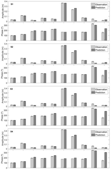
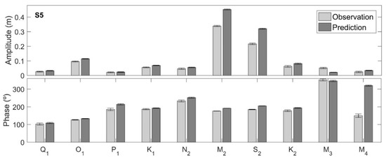
Figure 4.
Harmonic constants (amplitude (m) and phase (°)) determined from model predictions and observations, with error bars in the tidal gauges located in the Santos estuary.
Relative to the first station (S1), the main constituent, M2, is well reproduced, presenting an amplitude error of 0.21 cm and a phase lag of 6.48° (13 minutes). Highest discrepancies are found for S2 (amplitude error of 2.84 cm and a phase lag of 9.11° (18 minutes)), M3 (3.14 cm and comprehending a phase lag of 22.94° (32 minutes)) and M4 (1.51 cm with a phase lag of 83.82° (1h27 minutes)) constituents. For S2 constituents, discrepancies appear to be related to boundary conditions imposed, since predictions are higher than observations at the S1 station. For the M3 constituent, model underestimation of amplitude may reflect global astronomical solution uncertainties related to Brazilian regional features. It is important to mention that regarding the S3, S4 and S5 stations, M3 is the sixth most important constituent, proving this constituent amplification importance on the Brazilian coast. Regarding M4, the model overestimates the amplitude from the bay entrance. Further errors may reflect the bathymetric issues or arise from M2 uncertainties. Regarding diurnal constituents, very good agreement is found in terms of amplitude and phase lag, except P1 constituent presenting a phase lag of 19.8° (1hr19 minutes), being this lag amplified throughout the inner estuary. Generally, phase lags and amplitude differences increase towards S5.
The sum of amplitudes and relative importance of the main long period (6), diurnal (21), semi-diurnal (17), third-diurnal (5), quarter-diurnal and other shallow water constituents are presented in Table 5. These values correspond to the five tidal gauges (observations) and comprehend the 68 tidal constituents determined by the harmonic analysis performed.
Table 5.
Sum of the amplitudes (m) and relative importance (%) of the main tidal constituents in different frequency bands.
The amplification of total tidal harmonics is notable, from 1.49 m (S1) until 1.80 m (S4), except for the station S5, where a decrease was found. Regarding station S1, diurnal and semi-diurnal constituents are responsible for approximately 74% of the tidal energy in the Santos estuary. The significance of M2 in terms of amplitude is ~44% for all semi-diurnal constituents considered (results not shown). The significance of third-diurnal and quarter diurnal constituents is noticeable, being M3 responsible for 40% of total third-diurnal, whilst M4 contributes with 29% total quarter-diurnal amplitudes (results not shown). The importance of the non-linear terms by the amplification of third and quarter-diurnal constituents throughout the Santos estuary is clearly observed. A similar pattern was reported by [10] for the Paranaguá estuarine system. The harmonic analysis results (Figure 5) show HC intensification as the distance to the estuary mouth increases, regarding predictions and observations. This can be explained by the bathymetric uncertainties in the vast inter-tidal mangrove area of the inner estuary.
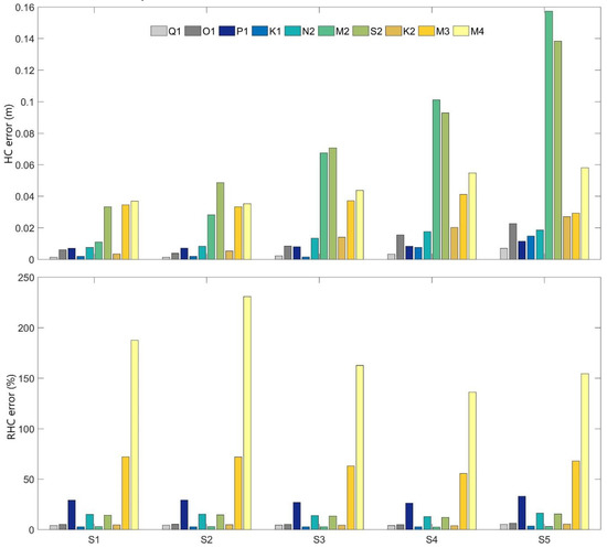
Figure 5.
Mean complex amplitude error (HC, top) in m and Relative mean complex amplitude error (RHC, bottom) in % error for the 5 tide gauges in Santos estuary for 2016–2017 using FES2012.
The major constituents portray the higher discrepancies between predictions and observations, namely M2 reaches a maximum difference at S5 (0.157 cm). HC values at S1 are less than 0.02 cm for the main constituents, except for S2 (0.33 cm) and for the shallow water constituents M3 and M4 (0.34 cm and 0.36 cm, respectively). Relative to RHC, major errors were found for the main non-linear constituents (M3 and M4). In general, for higher amplitude constituents, amplitude and phase difference between observations and predictions are lower. Moreover, differences in phase are observed for the shallow water constituents. This analysis concluded the main harmonics are reasonably reproduced since RHC are less than 10%. Conversely, for constituents P1 (RHC > 30%), M3 (RHC > 50%), and M4 (RHC > 130%) the largest discrepancies were found. These results show in a clear way that for the FES2012 the M3 and M4 present a large error in the coastal area (MOHID boundary).
3.3. Residual Tide Analysis
The statistical analysis to evaluate model performance in terms of the determined residual component (predictions and observations), for 2016–2017, is depicted in Table 6, including R, UNBIAS RMSE and S parameters.
Table 6.
Statistical parameters (R, UNBIAS RMSE, and S) (cm) for residual tide determined for the 5 tide gauges in Santos estuary for 2016–2017.
The statistical analysis was performed to understand the residual error variability towards the estuary. It can be observed that UNBIAS RMSE remains practically constant along with stations, between 9.48 cm and 12.1 cm in S5 and S3, respectively. R values oscillate between 0.85 (S5) and 0.91 (S4), whereas S values are comprehended between 0.90 (S1) to 0.92 (S2, S3, S4) respectively. The fact that the residual UNBIAS RMSE along the estuary does not show significant differences can reveal that major errors may be related to the astronomic tide. On the other hand, if predictions are improved on the Santos bay, this enhancement will be reflected towards the estuary. In the coastal zone of São Paulo, outside the estuary, the dynamics of sub-inertial atmospheric forced events are dominant, with time scales that vary between 4 and 8 days [8]. For the study area, the residual tide has the same magnitude order of the astronomic tide. However, the period is an order of magnitude greater. The celerity of both inside the estuary can be assumed equal. Consequently, the astronomic tide will have a smaller wavelength and stronger water level gradients and currents. In this case, the non-linear terms (bottom friction, advection, and mass balance) will distort more the astronomic tide along the Santos estuary rather than the residual one. This causes the astronomic tide to be more sensitive to errors in the bathymetry. Considering the constant residual errors in the estuary, an effort was made to improve predictions at Santos bay.
3.4. Influence of Oceanic Boundary Conditions
3.4.1. FES2014 Solution
The results of the model simulation using FES2014 solution with observations, in terms of the astronomical tide is presented in Figure 6.
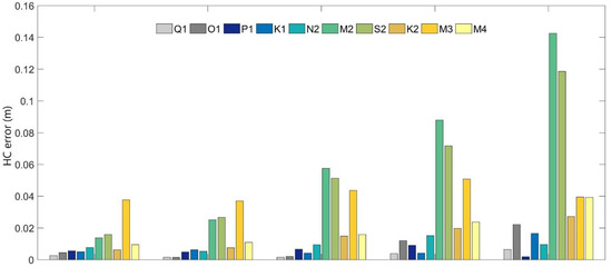
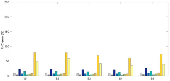
Figure 6.
Mean complex amplitude error (HC, top) in m and Relative mean complex amplitude error (RHC, bottom) in % error for the 5 tide gauges in Santos estuary for 2016–2017 using FES2014.
Compared to Figure 5, which considers FES2012 solution, it is shown that using FES2014 as an oceanic boundary condition leads to better results among different constituents. The best improvement is verified for M4 constituent regarding amplitude and phase values (RHC < 30%), considering the statistical parameters applied. There is a slight improvement in S2 constituent. The M3 inaccuracies are not solved with FES2014.
3.4.2. Copernicus Marine Environment Monitoring Service (CMEMS) Hourly Solution
The statistical analysis comparing the MOHID results using as open boundary reference solution hourly CMEMS water level shows a decrease of RMSE error of the water-level forecast in approximately 1 cm relatively to the configuration where CMEMS daily average are used. However, under extreme events the improvement is more notable. In these cases, the model is better able to capture the maximum water level values observed which have major importance for forecasting floods. A straightforward method to explain this improvement is a direct comparison of the S1 station meteorological tide with the CMEMS daily and hourly solutions. Figure 7 portrays hourly and daily residual tide provided by CMEMS with the residual tide (observed) for the S1 station and for three distinct time periods (18/04/2016 to 08/05/2016; 10/08/2016 to 28/08/2016; 15/09/2016 to 05/10/2016).
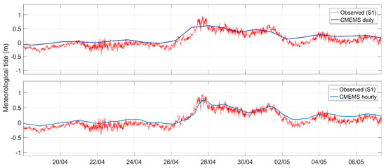
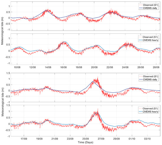
Figure 7.
Residual tide observed for the S1 station (observations) and Copernicus Marine Environment Monitoring Service (CMEMS, predicted): daily and hourly resolution for 3 distinct time periods (18/04/2016 to 08/05/2016; 10/08/2016 to 28/08/2016; 15/09/2016 to 05/10/2016).
It is evident that hourly CMEMS resolution better describes the observed residual tide, particularly the positive peaks (e.g., 27/04 and 26/09). Strong residual tide events were chosen, to better compare the use of distinct temporal resolutions. The hourly solution, used as an oceanic boundary condition in the model setup, improves the forecast capacity under extreme events comparing to the daily solution. Whilst the present study was ongoing, the CMEMS did not provide hourly barotropic velocities, only hourly water-level data. The previous implementation excelled at consistency in the open boundary and consequently the use of daily average water level and barotropic velocities used as reference solutions. Nevertheless, one of the performed tests included the use of barotropic velocity daily average together with the hourly water-level reference solutions. Despite the timeframe inconsistency, the results improve significantly under extreme events.
3.5. Investigating Wave Influence on Residual Tide Errors
Observations of positive residual tide compared to significant wave height evolution led to a working hypothesis that waves may influence the water level values (e.g., wave setup, wave-currents interaction), under storm conditions. Figure 8 portrays the pronounced correlation among residual tide and significant wave height.
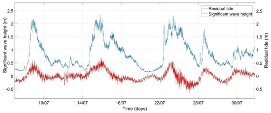
Figure 8.
Comparison between observed significant wave height and residual tide determined for S1 station.
Thus, the statistical analysis correlation between significant wave height (observed) and residual tide (predicted and observed) was assessed for the 5 tide gauges of the Santos estuary. Table 7 presents a pronounced correlation between residual tide (predicted and observed) and significant wave height (observed), being the maximum found in S2 (0.65).
Table 7.
The correlation coefficient (R) between residual tide (predictions and observations) and Hs (observation).
Correlations are higher for residual tide observations compared with residual tide predictions. From this analysis, it was concluded that the correlation estimated is not mainly related to the direct action of waves, because the correlation is also found in the predictions, which do not consider the wave effect in model implementation. However, the correlation is higher in the observations (~0.64) than in the predictions (~0.61), which might indicate that a second order effect, directly associated with the waves’ influence, may occur in the observations that it is not being considered in simulations. Therefore, the occurrence of extreme events was investigated (considering Hs higher than 1.5 m), and their possible effect on the residuals. Water level forecast errors are calculated once Hs is higher than 1.5 m. Table 7 shows residual tide UNBIAS RMSE for total time series (2016–2017) which is 12.10 cm and the UNBIAS RMSE for the indexes of Hs > 1.5, being 23.77 cm. This proves that forecast errors increase ~11.67 cm during storms.
Post-Processing Correction
Regarding the analysis period, 2016–2017, a total of 25 events of significant peak wave were estimated. The established threshold consisted of heights greater than 1.5 m leastwise 3 hours. Regarding each of the 25 events, the maximum height peak observed was calculated as well as the corresponding maximum value of observed and predicted residual. Afterward, the error (residual predicted minus residual observed) was calculated for each event. Table 8 displays the values of significant wave height and respective error, ascending orderly.
Table 8.
Statistical analysis (UNBIAS RMSE) of the residual tide (cm) for total time series and for Hs higher than 1.5 m.
Generally, for increasing values of Hs, residuals observations are higher, unlike for the predictions of residuals. For the extreme Hs events (maximum heights of 4.01 and 4.25 m), the highest errors were found (0.356 and 0.496 cm). A regression technique was applied, considering the Hs and residual error the independent and dependent parameters, respectively (Figure 9).
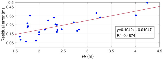
Figure 9.
Linear regression between Hs (m) and residual error (m).
Having the equation of the straight line, the sum of the slope coefficient (which is 0.1042 in this particular case) to the water level forecasts (once observed Hs is higher than 1.5 m) was tested, through the following equation:
where WL represents the Water Level, m is the slope coefficient and is the observed significant wave height.
The appliance of the correction factor statistical analysis is shown in Table 9, where the water level forecasts UNBIAS RMSE, during high wave activity, with and without the correction factor can be compared:
Table 9.
Statistical analysis (UNBIAS RMSE) of the residual tide for Hs higher than 1.5 m with and without correction factor.
The application of the correction factor improved the results in 11.67 cm, decreasing the UNBIAS RMSE from 23.77 to 12.10 cm. Figure 10 represents the correction applied for the period 2016–2017 for the model, model correction, observation, and Hs indexes higher than 1.5 m.
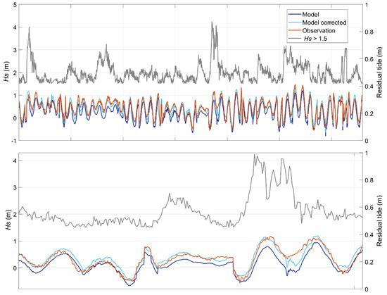
Figure 10.
Indices of Hs (grey) higher than 1.5 m, model predictions (dark blue), the model with a correction factor (light blue) and observations (orange) of the residual tide for the year of 2016–2017.
Analyzing Figure 10, it can be deduced that model correction (light blue line) values are nearer to observations (orange line). The regression technique applied comprehends forecasting residual tide using the direct inclusion of significant wave height data during storms. This assumes that non-periodic residual tide in the future will occur under similar meteorological conditions in history.
4. Conclusions
The tidal propagation presents a strong amplification occurring for most constituents regarding all stations analyzed along the Santos Estuary. The same pattern is verified for observations; however, an amplitude decrease was found for the station S5. Model validation was performed for the years 2016–2017, where errors ranged from 12.5 cm to 19.7 cm. Harmonic analysis briefly portrayed the model errors’ increase towards the inner estuary and the misrepresentation of M3 constituent, which is a very particular feature of the Brazilian shelf. Nevertheless, residual errors do not show significant differences along the Santos estuary. The individual study of water level components allowed the improvement of the forecast capacity for each component (astronomic and residual).
Concerning the astronomical features, upgrading the global tide solution from FES2012 to FES2014 resulted in several improvements in the astronomical boundary forcing, which optimized the harmonic predictions (e.g., S2 and M4 constituents). However, some inaccuracies persist (e.g., M3 constituent), as errors remain in shallow waters.
For the residual component, two hypotheses were tested, either improving the meteorological oceanic boundary (based on the CMEMS global solution) or assessing the possibility to correct data results in the post-processing stage. The implementation of an hourly instead of daily temporal resolution decreased the errors, improving the forecast capacity of extreme events in the Santos estuary. An upcoming stage includes the forecast system update to the hourly barotropic velocity (currently available for download at CMEMS). Additionally, the methodology developed for water-level increment detection allowed a post-processing correction, proving its efficiency in operational oceanography.
Some limitations remained which should be addressed in the future, such as bathymetric uncertainties, unsatisfactory spatial and temporal meteorological data resolution and the lack of river discharge data which makes freshwater input calculation for the Santos estuary difficult.
Problems related to astronomical tide inside the Santos channel appear to be mainly due to limitations of the bathymetric data available for the present area. Large discrepancies between observed mean water level of the tidal gauges show the potential lack of accuracy in the bathymetry referential, therefore better-quality bathymetric data is crucial to improve the model accuracy in the inner estuary.
In conclusion, for the present AQUASAFE implementation, the use of the FES2014 global solution in the oceanic astronomic boundary condition for MOHID setup is suggested, since it shows better results at the tide gauges closer to the inlet. Additionally, it is recommended to use the CMEMS hourly resolution as an oceanic meteorological boundary condition for MOHID application since it describes the residual tide positive peaks better.
Author Contributions
Conceptualization—J.M., P.L. and J.M.D.; data curation, —J.M. and P.L.; formal analysis—J.M.; funding acquisition—J.M.D. and J.C.L.; investigation—J.M. and P.L.; methodology—J.M., P.L., J.C.L., S.B., J.M.D.; project administration—P.L. and J.C.L.; resources—P.L., J.C.L. and J.M.D.; software—J.M., P.L., S.B., J.R.; supervision—J.C.L. and J.M.D.; validation—J.M.; visualization—J.M.; writing—original draft preparation—J.M.; writing—review and editing—P.L., J.C.L. and J.M.D.
Funding
Thanks are due for the financial support to CESAM (UID/AMB/50017-POCI-01-0145-FEDER-007638) to FCT/MCTES through national funds (PIDDAC), and the co-funding by the FEDER, Portugal, within the PT2020 Partnership Agreement and Compete 2020. The work done by authors affiliate with HIDROMOD was financed by the HiSea project funded by European Union’s Horizon 2020 research and innovation programme under grant agreement No 821934.
Acknowledgments
A special thanks to Santos Pilots for providing the access to atmospheric, wave and tidal gauge observations. Additional thanks to UNISANTA for providing the bathymetric data ready to be used by the model and for the discussions related to the best downscaling strategy to be followed.
Conflicts of Interest
The authors declare no conflict of interest. The funders had no role in the design of the study; in the collection, analyses, or interpretation of data; in the writing of the manuscript, or in the decision to publish the results.
References
- Mateus, M.; Giordano, F.; Marín, V.H.; Marcovecchio, J. Coastal zone management in South America with a look at Three Distinct Estuarine Systems. In Perspectives on Integrated Coastal Zone Management in South America; IST PRESS: Lisbon, Portugal, 2008; pp. 43–58. [Google Scholar]
- Kourafalou, V.; De Mey, P.; Staneva, J.; Ayoub, N.; Barth, A.; Chao, Y.; Cirano, M.; Fiechter, J.; Herzfeld, M.; Kurapov, A.; et al. Coastal Ocean Forecasting: Science foundation and user benefits. J. Oper. Oceanogr. 2015, 8, 147–167. [Google Scholar] [CrossRef]
- Leitão, J.; Galvão, P.; Leitão, P.; Silva, A. Operational Maritime Weather Forecast for Port Access and Operations Using the Aquasafe Platform. In Proceedings of the PIANC-COPEDEC IX, Rio de Janeiro, Brasil, 16–21 October 2016. [Google Scholar]
- Mancuso, M.; Ferreira, J.P.; Filho, J.L. Using GIS and Modeling to Assess Groundwater Discharge to Santos Estuary, Brazil, 2007; Technical Report, 9. Available online: https://www.researchgate.net/profile/Joao-Paulo_Lobo-Ferreira/publication/242113513_Using_GIS_and_modeling_to_assess_groundwater_discharge_to_Santos_Estuary_Brazil/links/54196a6f0cf25ebee98855f1/Using-GIS-and-modeling-to-assess-groundwater-discharge-to-Santos-Estuary-Brazil.pdf (accessed on 8 December 2019).
- Braga, R.R.; Leitão, J.C.; Leitão, P.C.; Puia, H.L.; Sampaio, A.P.F. Integration of high-resolution metocean forecast and observing systems at Port of Santos. In Proceedings of the PIANC—COPEDEC IX, Rio de Janeiro, Brazil, 16–21 October 2016; p. 13. [Google Scholar]
- Miranda, L.B.; Olle, E.D.; Bérgamo, A.L.; Silva, L.D.S.; Andutta, F.P. Circulation and salt intrusion in the piaçaguera channel, Santos (SP). Braz. J. Oceanogr. 2012, 60, 11–23. [Google Scholar] [CrossRef]
- Santos Port Authority. Available online: www.portodesantos.com.br (accessed on 10 October 2019).
- Chambel, J.; Mateus, M. D2. 3—Calibration of the Hydrodynamic Model for the Santos Estuary, 2008; Technical Report, 35. Available online: https://www.researchgate.net/profile/Ramiro_Neves/publication/238759899_D23_-_Calibration_of_the_hydrodynamic_model_for_the_Santos_Estuary/links/54a1777d0cf256bf8baf71c0.pdf (accessed on 8 December 2019).
- Huthnance, J.M. On natural oscillations of connected ocean basins. Geophys. J. Int. 1980, 61, 337–354. [Google Scholar] [CrossRef]
- Franz, G.A.S.; Leitão, P.; dos Santos, A.; Juliano, M.; Neves, R. From regional to local scale modelling on the south-eastern Brazilian shelf: Case study of Paranaguá estuarine system. Braz. J. Oceanogr. 2016, 64, 277–294. [Google Scholar] [CrossRef]
- Lopes, P.G. As Assimetrias de Maré no Estuário de Santos—SP, Brasil. Ph.D. Thesis, Universidade Federal do Rio de Janeiro, Rio de Janeiro, Brazil, 2015. [Google Scholar]
- Campos, R.M.; Camargo, R.; Harari, E.J. Caracterização de eventos extremos do nível do mar em Santos e sua correspondência com as reanálises do modelo do NCEP no sudoeste do Atlântico Sul. Rev. Bras. Meteorol. 2010, 25, 175–184. [Google Scholar] [CrossRef]
- Agência FAPESP. Available online: http://agencia.fapesp.br/inundacoes-costeiras-em-santos-podem-causar-prejuizos-bilionarios/21997/ (accessed on 5 November 2017).
- Harari, J.; Camargo, R. Estimation of the volume transport by the tides in the south-eastern Brazilian platform through a hydrodynamical model. In Proceedings of the II Simpósio Sobre Ecossistemas da Costa sul e Sudeste Brasileira: Estrutura, Função e Manejo, Águas de Lindóia, Brazil, 6–11 April 1990; pp. 75–83. [Google Scholar]
- Moser, G.A.O. Aspectos da Eutrofização no Sistema Estuarino de Santos: Distribuição Espaço-Temporal da Biomassa e Produtividade Primária Fitoplanctônica e Transporte Instantâneo de Sal, Clorofila-a, Material em Suspensão e Nutrientes. Ph.D. Thesis, Universidade de São Paulo, Instituto Oceanográfico, Brasil, 2002. [Google Scholar]
- Castro, B.M.; Lee, T.N. Wind-forced sea level variability on the southeast Brazilian shelf. J. Geophys. Res. 1995, 100, 16045–16056. [Google Scholar] [CrossRef]
- Harari, J.; França, C.; Camargo, R. Climatology and hydrography of Santos estuary. In Perspectives on Integrated Coastal Zone Management in South America; IST PRESS: Lisbon, Portugal, 2008; pp. 147–154. [Google Scholar]
- Santos, A.J. Modelo Hidrodinâmico Tridimensional de Circulação Oceânica e Estuarina. Ph.D. Thesis, Universidade Técnica de Lisboa, Lisbon, Portugal, 1995. [Google Scholar]
- Leitão, P. Integração de Escalas e Processos na Modelação do Ambiente Marinho. Ph.D. Thesis, Universidade Técnica de Lisboa, Lisbon, Portugal, 2003. [Google Scholar]
- Vaz, N. Study of Heat and Salt Transport Processes in the Espinheiro Channel (Ria de Aveiro). Ph.D. Thesis, Universidade de Aveiro, Aveiro, Portugal, 2007. [Google Scholar]
- Leitão, P.; Coelho, H.; Santos, A.; Neves, R. Modelling the main features of the Algarve coastal circulation during July 2004: A downscaling approach. J. Atmos. Ocean. Sci. 2005, 10, 421–462. [Google Scholar]
- Carrère, L.; Lyard, F.; Cancet, M.; Guillot, A.; Roblou, L. FES2012: A new global tidal model taking advantage of nearly 20 years of altimetry. In Proceedings of the 20 Years of Altimetry, Venice, Italy, 24–29 September 2013; p. 6. [Google Scholar]
- Lellouche, J.; Regnier, C. Global Ocean Sea Physical Analysis Forecasting Products. In Product User Manual. 2015, p. 16. Available online: http://resources.marine.copernicus.eu/documents/PUM/CMEMS-GLO-PUM-001-002.pdf (accessed on 8 December 2019).
- Pawlowicz, R.; Beardsley, B.; Lentz, S. Classical tidal harmonic analysis including error estimates in MATLAB using T_TIDE. Comput. Geosci. 2012, 28, 929–937. [Google Scholar] [CrossRef]
- Chanut, J.; Galloudec, O.L.; Léger, F. Towards North East Atlantic Regional modelling at 1/12° and 1/36° at Mercator Ocean. Mercator Ocean Q. Newsl. 2010, 34, 4–12. [Google Scholar]
- Pugh, D. Tides, Surges and Mean Sea-Level; John Wiley & Sons: Chichester, UK, 1987; p. 472. [Google Scholar]
- Horsburgh, K.J.; Wilson, C. Tide-surge interaction and its role in the distribution of surge residuals in the North Sea. J. Geophys. Res. 2007, 112. [Google Scholar] [CrossRef]
- Pugh, D.; Woodworth, P. Sea-Level Science: Understanding Tides, Surges, Tsunamis and Mean Sea-Level Changes; Cambridge University Press: Cambridge, UK, 2014; p. 395. [Google Scholar]
- Dias, J.; Lopes, J. Calibration and validation of hydrodynamic, salt and heat transport models for Ria de Aveiro lagoon (Portugal). J. Coast. Res. 2006, III, 1680–1684. [Google Scholar]
- Oliveira, M.D.; Ebecken, N.F.; Santos, I.D.A.; Neves, C.F.; Caloba, L.P.; de Oliveira, J. Modelagem da maré meteorológica utilizando redes neurais artificiais: Uma aplicação para a Baía De Paranaguá—Parte 1: Dados meteorológicos da estação de superfície. Rev. Bras. Meteorol. 2006, 21, 220–231. [Google Scholar]
- Willmott, C.J. On the validation of model. Phys. Geogr. 1981, 2, 184–194. [Google Scholar] [CrossRef]
- Dias, J.M.; Sousa, M.C.; Bertin, X.; Fortunato, A.B.; Oliveira, A. Numerical modeling of the impact of the Ancão Inlet relocation (Ria Formosa, Portugal). Environ. Model. Softw. 2009, 24, 711–725. [Google Scholar] [CrossRef]
- Aviso+—Satellite Altimetry Data. Available online: www.aviso.altimetry.fr (accessed on 5 May 2018).


© 2019 by the authors. Licensee MDPI, Basel, Switzerland. This article is an open access article distributed under the terms and conditions of the Creative Commons Attribution (CC BY) license (http://creativecommons.org/licenses/by/4.0/).