Hydropower Dam State and Its Foundation Soil Survey Using Industrial Seismic Oscillations

Abstract

In this article, we suggest a new type of seismic source for surveying both structure state and foundation soil conditions regardless of the level of seismic noise. In our opinion, powerful industrial equipment can be treated as seismic sources. We describe the results of a survey conducted on the Song Tranh-2 hydropower dam located in Central Vietnam. After a М = 4.7 earthquake, the dam visual inspection revealed zones of the excessive durability loss: cracks and areas with an elevated infiltration of water into the dam galleries. Powerful industrial equipment generates continuous quasi-harmonic mechanical oscillations (seismic waves) that travel through layers of rocks. These seismic oscillations are recorded by receivers in different measurement points such as the dam body, abutments, and the foundation soils. Anomalous amplitudes of these oscillations indicate the presence of weakened zones in the structure or in foundation soil. We coupled passive and active seismic methods to more precisely find such zones. In this case, active seismic methods allowed us to investigate dam abutment zones, and passive seismic methods were used to localize weakened zones in the dam-foundation soil system. We assumed that the joint contribution of two factors was the cause of the dam weakening. One of them was caused by increased water infiltration through the rock mass and its contact zones, and the other was reservoir-induced seismicity contributing to the deterioration of the foundation soils, which was possibly the reason for a shift in the dam in the contact zone with the rock mass foundation. It is necessary to perform computer modelling, which was not included in our research. The developed method can be used for the safety control of the hydropower station dams.

1. Introduction

The goal of structural health monitoring techniques is to identify, quantify, and locate damage as well as to determine the possible causes of structural damage. According to previous studies [1,2], the strength reduction of the object state is directly related to the appearance of defects in the foundation soil. Therefore, to determine the sources of damage, it is important to survey both the structure’s state and its foundation soil condition. For these purposes, both active and passive seismic control methods and ambient vibration testing along with their complexing can be implemented [3,4,5,6,7,8,9].

The advancement of seismic equipment and the development of a methodological base have led to the passive seismic methods and ambient vibration testing becoming increasingly important in structural health and safety monitoring [10,11,12,13,14]. If, for some passive seismic methods that are based on the cross-correlation or convolution of ambient noise, a high level of microseisms is necessary [15,16,17]. For other methods that determine the natural frequency of a structure [3,10,18] or are based on spectral analysis of the natural ambient seismic noise [19,20,21], a high level of microseisms is a negative factor that impedes the data processing. Each of these methods has its own requirement for seismic noise level and frequency range, which is why coupling these methods in one experiment is difficult or sometimes impossible. For example, methods based on the cross-correlation or convolution of the signals requires accurate time synchronization between all seismic sensors, which is hard to implement inside the body of a structure. To do this, it is necessary to use data loggers with high-precision generators, which may not be available. We aimed to expand the capabilities of seismic methods in object state surveys. In our opinion, treating powerful industrial equipment as seismic sources provides the opportunity to survey both the structure state and foundation soil condition regardless of the level of seismic noise. These kind of seismic sources can provide continuous flows of energy and generate seismic waves that propagate through medium, such as a dam or layers of rocks, and are detectable at any point in the investigated area. The positive aspects of this survey are: (1) the observation system may consist of few seismic sensors that are consistently relocated across the construction and the geological media, and (2) the possibility of monitoring at any time without the need for a specific active seismic source by using only ambient seismic noise including industrial oscillations.

We implemented these ideas to survey the Song Tranh-2 HPP dam (Central Vietnam) and used both passive and active seismic methods to control the results.

2. Research Object Description

The Song Tranh-2 concrete gravity dam is located in Central Vietnam in Quang Nam province. The dam is 80 m in height and 640 m in length; the cross-section is triangle-like with inner galleries (Figure 1a). The deterioration of the dam is visible with the naked eye (Figure 1b) [4]. For the further usage of the dam, it was necessary to assess how the surface defects were affecting the dam body state and to identify the cause of the structural deterioration using passive seismic methods because of the difficulties in applying ambient vibration testing methods. We completed state surveys for these objects: dam body, its abutments, and the foundation soil.

2.1. Geological and Geophysical Characteristics of the Investigated Area

General information about the foundation soil (Figure 2) was obtained before construction of the dam by an engineering-geological survey and was kindly provided by our colleagues at the Institute of Geophysics of the Vietnam Academy of Science and Technology (VAST). The riverbed is inside a grabenoid structure, containing plentiful cracks oriented toward the center of the graben. The upper part of the geological section consists of quaternary sediments (edQ) with clay, sand, and gravel; below are the weathered rocks and (IA1, IA2) cracked rocks of the basement (IIA). The rocks of the basement (IIB, PR_2-3) are represented by gneisses, amphibolites, shales, gabbros, diorites, migmatites, and granites, etc.

The area around the dam has a complex geological structure and exhibits geodynamic activity in the form of frequent earthquakes with variable magnitudes [22]. Both sides of the river plain are crossed by north-east and north-west cracks (along the river flow). The direction of the rock cracking (azimuth 160–170°) is inherent for both regional and local zones (Figure 3). Notably, small cracks are close to vertical, meaning that they can transmit fluid into the deep layers, thus activating geodynamic processes of reservoir-induced seismicity. Similar behavior was observed for Nurek Hydro Power Plant (HPP) and is generally well-known [23].

In 2011, the reservoir filling was accompanied by an intense burst of shallow seismic activity. The results of preliminary investigations indicated that this seismic activity was reservoir induced [22]. After an earthquake with magnitude of 4.7, the water level in the lake lowered to the minimum. The subsequent visual inspection revealed zones of excessive durability loss: cracks and areas with an elevated infiltration of water into the dam galleries. The latter was aggravated by concrete defects all across the reservoir side surface of the dam (Figure 1b). The defects are concentrated in the lower part, often forming extended zones.

The design of Song Tranh-2 is tailored to withstand earthquakes up to M = 5.5. The calculated seismic impact response used for design shows that (1) all parts of the dam are moving when exposed to vibration, especially the upper part (upper third of the dam), and thus the most damage is expected to happen there and (2) the foundation soil is also susceptible to vibrations. The latter implies that an inspection of the soil state should be conducted regularly after the construction was complete. So, complex seismic inspections must cover both dam and its foundation soil.

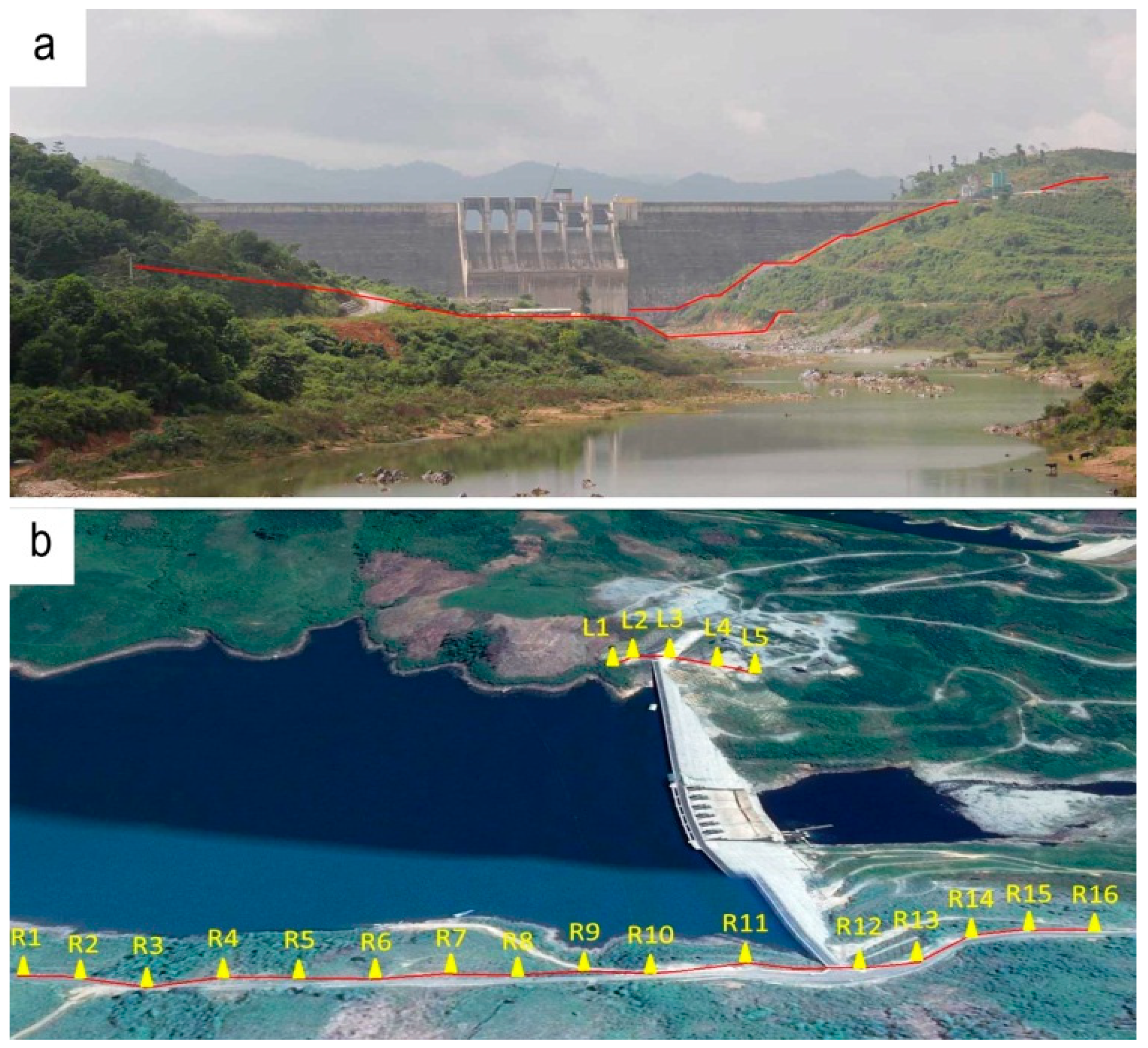
2.2. Seismic Equipment and Observation Scheme

We conducted the seismic survey during two field seasons in one-year intervals. In the first stage of work, we used equipment belonging to the Institute of Geophysics VAST including four analogue seismometers CMG-40T by Güralp Systems Ltd. (city, UK) with SAMTAC-801H data loggers (Japan). The frequency range was 0.1 to 50 Hz and the dynamic range was 130 dB. The time reference is global positioning system (GPS)-based except for the measurements inside the dam, where the internal sensor clocks were used. In the second stage of the study, we used 7 sets of digital seismometers CMG-6TD (Güralp Systems Ltd.). We recorded several successive profile measurements: along the dam’s ridge and then along first, second, and third galleries. Each profile had an immobile reference station in the center of the dam [4].

We used the same set of equipment for ambient seismic noise recording in the dam area. A long measurement profile (Figure 4a) was parallel to the dam’s foundation, 250 m away from it. Figure 4b shows the detailed observation scheme for river banks in the second stage of the work. The distances between measurement points closest to the dam area were 20–30 m, then 40–50 m, and reaching 100 m for the most distant point. The choice of such placement was dictated by the equipment placement conditions.

In addition, we used active shallow seismic survey (24-channel station Geode [24]) for complex interpretation of the results together with passive seismic methods. Probing waves originated from 8 kg sledgehammer strikes on the steel plate; we studied pick-ups seismic P- and S- waves at horizontal and vertical components. The schematic chart of the shallow seismic survey is shown in Figure 5. The spacing between channels was 1, 2, 3, and 5 m and the corresponding profile lengths were 24, 48, 72 and 120 m. Signals were processed with RadExPro+ [25] and ZondST2d [26] software suites with support from Geosignal Ltd. [27].

3. Survey Methods

3.1. The Sounding of Dam Structure and Ground by Signals from an Industrial Source

In our investigation, we used the method described in [4] as the main passive seismic method. In this method, artificial vibrations from industrial sources are used for the study of the dam state and upper crust in the area of its location. In the 1980s, many scientific studies were devoted to the propagation and extraction of quasi-harmonic signals from microseisms using electrical equipment [28,29,30,31]. This type of signal was also used to investigate the Earth’s crust. Such artificial signals are clear in the microseisms power spectra as linear peaks at frequencies f = 50/n, where 50 Hz is the electric network frequency and n is the number of pairs of electrical motor poles. A few examples are shown in Figure 6.

These signals are notable due to the frequency variation in time occurring due to the frequency value depending on the temporal variation of the electrical network frequency. The typical time interval of industrial frequency stability is tens of minutes; therefore, to extract seismic vibration signals from ambient seismic noise at distances under about 5 km, it is sufficient to perform a computation of microseism power spectral density function with desired frequency resolution. At distances of more than tens of kilometers, it is necessary to use a tracking filter with electric power network as a reference signal [23]. As the signals from industrial equipment are continuous quasi-harmonic signals, it is possible to estimate the amplitudes values of these signals at different measurement points with desired signal-to-noise ratio.

In our case, the distance from the operating industrial device was about 1 km; therefore, we could extract a signal by calculating the microseisms power spectral density function (PSD). PSD is computed by averaging of a number fast Fourier transform (FFT) estimations for half-interval time overlapping and smoothing. Figure 7 shows the typical PSD at one of the points inside the Song Tranh-2 dam. As we analyzed the spatial distribution of amplitude at a specific frequency, we take the square root of the PSD. Amplitude values of industrial signals are determined by a number of technological factors and may change quite quickly (up to ten minutes), but the ratio of the amplitude at the ith point to the reference unmovable point (A_i/A₀) was used to correct the temporal drift in the data. As a result, we only obtained the spatial variation in the amplitudes at the appropriate frequency. It is important to maintain the distance between the reference and measurement points to be comparable to the signal wavelength; so, in the case of frequency (wavelength) drift, the deviation of the amplitude ratios remains minimal. If these precautions are taken, the cumulative distortion of the spatial distribution of relative amplitudes is non-crucial. This is why we placed the reference point on the dam for its survey and on the ground for the geological environment survey.

The dam is long; its length on the crest is 8 times greater than the height, and an industrial pump works inside the dam. There is a road with intensive traffic near the dam. All these factors increase the level of microseismic noise and complicate attempts to determine the dam’s characteristic frequencies. However, industrial vibrations are clearly manifested in microseisms PSD as peaks with frequencies of 3.125 Hz and approximately 4.6 Hz. As at each stage we required about 10 days to survey the dam and its territory, we had to employ signals at these industrial frequencies to survey both the dam and its geological environment.

Inside the dam, the duration of measurements was 40 min at each point. When we surveyed the geological environment, we spent 1.5–2 h at each point. Anomalous amplitudes values indicated the presence of a weak zone (in the structure or foundation soil).

The microseisms records obtained during the survey of the geological environment were also processed by additional passive seismic analysis methods (microseismic sounding and temporal autocorrelation functions).

3.2. Microseismic Sounding Method

The description of the microseismic sounding method (MSM) along with some examples were provided in previous studies [5,34]. The MSM assumes that the vertical component of the natural microseisms is predominantly contributed by the fundamental Rayleigh modes, the contributions of the higher modes are insignificant, and the effects of these modes can be treated as noise. The basic informative parameter for MSM is the amplitude (intensity) of a signal. Phase data were not used [34].

The amplitude of the surface wave at a certain frequency (f) depends on velocity of its propagation in the geological environment; small velocities correspond to large amplitudes, and vice versa. This frequency f is linked to the depth of inclusion H and to the corresponding phase velocity of the fundamental Rayleigh mode V_R(f) via the following relationship:

H ≈ k_GV_R·(f)/f,

(1)

where the depth tying coefficient k_G is close to 0.4 [5,19]. An interpretation of the Rayleigh wave package at different frequencies provides the information about velocities at various depths. MSM targets the near-vertical inhomogeneities. The method has been adopted to fit various geological tasks and special software was developed for data processing in the field [35,36].

3.3. Temporal Autocorrelation Functions

This method treats periodical signals, their correlation, and their likeness at different time intervals [37,38]. It is based on the temporal signal correlation with itself, which is estimated by calculating time-dependent autocorrelation function [37]:

$$\mathsf{\Psi }\left(\tau \right)={{\displaystyle \int }}_{-\infty }^{\infty }f\left(t\right)f^{*}\left(t-\tau \right)dt,$$

(2)

where f(t) is a seismogram, τ is time shift, and * is a complex conjugation. This function characterizes the similarity of the signal to its own copy shifted by τ. The function local maxima correspond to phase-matches, whereas minima mark signals in the counter-phase.

This method is widely used in data processing when analysis of data series is necessary. In seismology, this method serves to extract information about deep reflectors from the coda of seismic phases [39,40]. Claerbout et al. [41] proposed the idea of using autocorrelation functions for the investigation of the subsurface.

In this article, we present the transmission properties of the dam and the zones of contact with geologic media obtained via the analysis of autocorrelation functions of the seismic noise, recorded along the right and left banks. We assumed that the dam is the source of a quasi-harmonic signal that can be recorded on both sides of the river. In this case, if transmission properties of the zones of contact are the same for both sides, the autocorrelation functions of signals recorded on different sides have to be the same. Differences in the correlation properties of signals are indicators of weak zones.

3.4. Active Seismic Methods

For the study of foundation soil and dam abutments, we used active shallow seismic survey including reflection and refraction methods and multichannel analysis of surface waves (MASW). These methods are based on different types of seismic waves characterized by different modes of propagation. The common feature of these methods is their sensitivity to spatial changes in seismic velocities in the subsurface [42]. The set of seismic data acquired at the surface was used to estimate the rocks velocity distribution and map the corresponding structural features. For this purpose, each method implements its specific acquisition and processing techniques. A short general overview of shallow seismic methods was provided by Steeples [43].

The MASW method is described in pioneering works [44,45,46] and was developed by Park et al. [47]. It investigates the dispersion properties of the surface waves and produces one-dimensional velocity models of the geologic media along linear seismic survey profiles. The core of the multichannel surface waves analysis technique is a wave-spectra (f − k) signal processing with the consecutive summarization across all channels [48,49].

4. Results

4.1. Sounding of Dam Structure by Signals from Industrial Source

Figure 8 shows the spatial distributions of amplitudes at 3.125 Hz obtained during the two field seasons with an interval of one year between them. We did not study wave nature (P-, S-, or surface) of industrial vibrations used for our transmission studies. Therefore, it is difficult to relate the obtained values to the propagation velocities of the seismic waves in the dam body. Nevertheless, the homogeneous spatial amplitude distribution corresponds to the homogeneous material, whereas anomalies mark zones with transformed properties. In the first field season, the left side of the dam had a bright anomaly (Figure 8a), which corresponds to an area with decreased durability. The visual inspection revealed wet walls inside the dam and water leaks. Some areas in the central part were starting to degrade (blue spots in Figure 8a). In the second field season, such observations were confirmed (Figure 8b): the left anomaly persisted and the dam exhibited a general loss in durability.

Let us consider the sounding results of the upper part of geological media near the dam using the industrial frequency of 3.125 Hz. The vertical component amplitude was normalized to one in stationary point and is presented in a logarithm scale (Figure 9). The results for the horizontal components were similar. Figure 9 shows that the right riverbank has two anomalies, one of which is in the abutment of the dam. High amplitude ratios may be explained by the weakening of the object (in this case, the geological environment) in this area, and we assumed rocks were fracturing in the areas. The left riverbank generally had a more homogeneous 3.125 Hz amplitude distribution, which indicates its stability.

4.2. Microseismic Sounding Result

The microseismic sounding of the upper part of the geological section revealed high-contrast near-vertical inhomogeneities related to the cracked structure of the rocks and the ruptured tectonics (Figure 10). The yellow-red spots mark low-velocity zones, probably weakened by cracks. Their position suggests that the area has a large multi-scale rupture system divided in blocks. Therefore, the deformation processes inside the block are more intense. The side joints of the dam ends exhibit non-equal velocity and thus unequal material strength properties. The left side is dense with higher velocities, while the other one is weakened due to velocities being lower.

4.3. Analysis of Autocorrelation Functions

As the dam is a source of a quasi-coherent signal in the time domain, the autocorrelation functions for seismograms at various distances from the dam provide some information about the geological structure. The transmission properties of the dam in Figure 11 were acquired by the processing the seismic noise recorded along the right and left side profiles (Figure 4b). The autocorrelation function for the left riverbank has a small correlation coefficient for the non-zero time lags compared to the right one, implying that the left riverbank has no specific signal source. A stable signal source is visible in the upper part of the section only in the right riverbank near dam abutment in Figure 11a, and the correlation coefficient decreased with distance from the right dam abutment. This occurred because the dam abutment zones have better transmission properties compared to other areas. This, in turn, signals a breach in the dam integrity at the right side contact zone.

4.4. Multichannel Surface Wave Analysis

We built two axis velocity models by inverting dispersion curves for profiles: PR13-21 (right side) and PR22-24 (left side), as in Figure 5. The low-velocity slab (ca. 200 m/s) of transversal waves was up to 5 m deep on the right side and extends 180–200 m from the dam with the depth reaching 15 m (Figure 12). The low-velocity zone on the left side exists only in the surface layer. Despite the velocity cross-section of the right side being more detailed due to having more profile points, it has a more mosaic-like structure compared to the left side. Low-velocity zones might be related to the water-saturated soils. Generally, the right side has higher density rarefaction and thus is less stable.

4.5. Active Shallow Seismic Survey

Based on the results of the shallow seismic surveys, we identified reflective and refractive seismic boundaries in the depth range from 0 to 26 m, which were compared to the stratigraphic boundaries and lithology according to the available information from wells (Figure 2). The velocity properties of layers for the most informative profiles are presented in

Table 1. Velocity properties of seismic layers for the most informative profiles.

Right River Bank					Left River Bank
Profile No.	Refracting Boundary	Layer Depth, H (m)	Vp (m/s)	Vref (m/s)	Profile No.	Refracting Boundary	Layer Depth, H, m	Vp (m/s)	Vref (m/s)
4, 5, 6	edQ/IAµ	2–10	500	1400	1, 2, 3	edQ/IAµ	2–10	330–400	1400
8	edQ/IAµ	3–9	374–622	970–1835
8	IA/IB	15–26	940–970	2500–3000
10–11	edQ/IAµ	8	400–800	1200–1600	25–26	edQ/IAµ	4–6	550–598	1410–2030
10–11	IAµ/IB	12–14	1000	2200–3000	25–26	IAµ/IIA	14–18	814–983	4430–5030
13	edQ/IAµ	6–15	263–346	606–1136	22–24	edQ/IAµ	4–6	518–650	1316–2270
21	IIA/IIB	9–13	1080–1180	2800–5100	24	IIA/IIB	15–18	1060–1133	3300–4600

with the indication of layer depth. As an example, the typical seismic cross-section for each riverbank is given: profile 8 for the right riverbank (Figure 13) and profile 24 for the left bank (Figure 14). Note the number of common patterns for both river banks.

For the upper part of the section (edQ), the thickness of the Quaternary sediment layer was represented by clays, sand, and gravel, varying from 2 to 5 m for the left riverbank and up to 8 m for the right bank. The average velocities of P waves (Vp) in this layer were up to 630 m/s.

The completed weathered rock (IAµ) layer, represented by clays, loams, and loamy sand with gravel, is about 30 m thick. The average value of the refractor velocity (Vref) was 1500 m/s. The faults were visible in a temporal field and could be distinguished by changing the velocities in the geo-seismic sections (Figure 13and Figure 14). On the right riverbank, we identified a zone of low velocities at about 1000 m/s (Figure 13) especially during the rainy season. Thus, rocks in this zone are characterized by a lower external load bearing capacity than the left riverbank.

The weathered rock (IB) layer is represented by gneisses, amphibolites, shales, gabbro, granodiorites, and diorites, and is characterized by high fragmentation of the geological environment. The refractor velocity for both sides ranges from 2500 to 3000 m/s.

The relatively intact rock (IIB) layer is located at depths from 20 to 30 m. The refractor velocities are within from 3900 to 5100 m/s as defined by the different lithology of foundation blocks.

Thus, we observed a slight difference in the velocities of geo-seismic sections for both riversides. We identified some faults zones in the foundation rocks that at 20–40 m depths (Figure 15, where the results of the previous methods are presented schematically). We assumed that the presence of fault series in the right dam abutment area may affect its fixation.

5. Discussion

We identified a weakened zone inside the dam on the left side and a weak zone in the right abutment by sounding with industrial seismic vibrations at 3.125 Hz. The weak zone of the right abutment was confirmed by the results of passive and active seismic methods. These results acknowledge the ability to consider the powerful operating industrial equipment as a seismic source that can help to rapidly survey the state of different objects. This method only detects weakened areas; for a more detailed study, it is necessary to use other methods. However, this reduces the amount of work, for example compared with active seismic methods or for structure state survey, as most of weakened areas where the greatest destruction in the future are expected were identified.

The jointing of passive and active seismic methods allowed us to identify the differences in rock deformation properties of the right and left riverbanks. The increased rock fracturing of the right riverbank, according to engineering-geological surveys, may cause an increase in the rocks’ stress-strain state in the right part more than in the left when the reservoir is filling. As most of the negative phenomena associated with gravitational dams are caused by increased water infiltration through the rock mass and its contact zones [50,51,52], we can assume that, in our case, this phenomenon is the cause of the observed deformation of the foundation soils properties. Reservoir-induced seismicity also contributed to the deterioration of the foundation soils, and possibly was the reason for a shift in the dam contact zone with the rock mass foundation. Both factors result in an alteration of the rock foundation strains producing cracks in the dam.

6. Conclusions

We obtained a good agreement between independent seismic methods that demonstrated that weakened foundation leads to disruptions in the dam body. Using this information before and after the dam repairs, it is possible to increase the safety of the hydropower station. Thus, it is important to conduct a survey of the structure–foundation soils system. Powerful industrial equipment can act as a seismic source that greatly simplify conducting surveys. This type of passive source of seismic vibrations extends the application possibilities of ambient vibration testing and passive seismic methods.

References

1. Pashkin, E.M.; Vyazkova, O.E. Role of engineering geology in the preservation of historical and cultural-heritage. Vestn. Ross. Akad. Nauk 1993, 63, 326–331. [Google Scholar]
2. Konovalov, P.A. Bases and Foundations of Buildings under Reconstruction; Balkema, A.A., Ed.; CRC Press: Rotterdam, The Netherlands, 1998. [Google Scholar]
3. Ivanovic, S.S.; Trifunac, M.D.; Todorovska, M.I. Ambient Vibration Test of Structures—A Review. ISET J. Earthq. Technol. 2000, 37, 165–197. [Google Scholar]
4. Antonovskaya, G.; Kapustian, N.; Ngo Thi, L. Seismic engineering investigation of hydropower station dams. In Proceedings of the 2nd European Conference on Earthquake Engineering and Seismology, Istanbul, Turkey, 25–29 August 2014; pp. 223–233. [Google Scholar]
5. Gorbatikov, A.V.; Tsukanov, A.A. Simulation of the Rayleigh waves in the proximity of the scattering velocity heterogeneities. Exploring the capabilities of the microseismic sounding method. Izv. Phys. Solid Earth 2011, 47, 354–369. [Google Scholar] [CrossRef]
6. Burger, H.R. Exploration Geophysics of the Shallow Subsurface; Prentice Hall P T R: Englewood Cliffs, NJ, USA, 1992. [Google Scholar]
7. Robinson, E.S.; Coruh, C. Basic Exploration Geophysics; John Wiley: Hoboken, NJ, USA, 1988. [Google Scholar]
8. Telford, W.M.; Geldart, L.P.; Sheriff, R.E. Applied Geophysics, 2nd ed.; Cambridge University Press: Cambridge, UK, 1990. [Google Scholar]
9. Adly, A.; Poggi, V.; Fah, D.; Hassoup, A.; Omran, A. Combining active and passive seismic methods for the characterization of urban sites in Cairo, Egypt. Geophys. J. Int. 2017, 210, 428–442. [Google Scholar] [CrossRef]
10. Trifunac, M.D. Comparison between Ambient and Forced Vibration Experiments. Earthq. Eng. Struct. Dyn. 1972, 1, 133–150. [Google Scholar] [CrossRef]
11. Buyukozturk, O.; Yu, T.-Y. Structural Health Monitoring and Seismic Impact Assessment. In Proceedings of the Fifth National Conference on Earthquake Engineering, Istanbul, Turkey, 26–30 May 2003. [Google Scholar]
12. Ebrahimian, M.; Todorovska, M.I.; Falborski, T. Wave method for Structural Health Monitoring: Testing using full-scale shake table experiment data. J. Struct. Eng. ASCE 2016, 143, 04016217. [Google Scholar] [CrossRef]
13. Antonovskaya, G.N.; Kapustian, N.K.; Moshkunov, A.I.; Danilov, A.V.; Moshkunov, K.I. New seismic array solution for earthquake observations and hydropower plant health monitoring. J. Seismol. 2017, 21, 1039–1053. [Google Scholar] [CrossRef]
14. Mirtaheri, M.; Salehi, F. Ambient vibration testing of existing buildings: Experimental, numerical and code provisions. Adv. Mech. Eng. 2018, 10. [Google Scholar] [CrossRef] [Green Version]
15. Cheng, F.; Xia, J.; Luo, Y.; Xu, Z.; Wang, L.; Shen, C.; Liu, R.; Pan, Y.; Mi, B.; Hu, Y. Multichannel analysis of passive surface waves based on cross correlations. Geophysics 2016, 81, 1–10. [Google Scholar] [CrossRef]
16. Draganov, D.; Campman, X.; Thorbecke, J.; Verdel, A.; Wapenaar, K. Reflection images from ambient seismic noise. Geophysics 2009, 74, A63–A67. [Google Scholar] [CrossRef]
17. Le Feuvre, M.; Joubert, A.; Leparoux, D.; Cote, P. Passive multi-channel analysis of surface waves with cross-correlations and beamforming. Application to a sea dike. J. Appl. Geophys. 2015, 114, 36–51. [Google Scholar] [CrossRef]
18. Kuzmenko, A.; Vorobyeva, D.; Zolotukhin, E. Monitoring the technical condition of dams of hydroelectric power plants with an automated monitoring and earthquake registration system. In Proceedings of the Power Engineering and Automation Conference, Wuhan, China, 18–20 September 2012. [Google Scholar] [CrossRef]
19. Gorbatikov, A.V.; Stepanova, M.Y. Statistical characteristics and stationarity properties of low-frequency seismic signals. Izv. Phys. Solid Earth 2008, 44, 50–59. [Google Scholar] [CrossRef]
20. Bhowmik, B.; Krishnan, M.; Hazra, B.; Pakrashi, V. Real-time unified single- and multi-channel structural damage detection using recursive singular spectrum analysis. Struct. Health Monit. 2019, 18, 563–589. [Google Scholar] [CrossRef]
21. Colombero, C.; Baillet, L.; Comina, C.; Helmstetter, A.; Jongmans, D.; Larose, E.; Valentin, J.; Vinciguerra, S. Spectral Analysis and Correlation of Ambient Seismic Noise. The Case Study of Madonna del Sasso (NW Italy). In Proceedings of the Conference: EAGE Near Surface Geoscience, 21st European Meeting of Environmental and Engineering Geophysics, Turin, Italy, 6–10 September 2015. [Google Scholar] [CrossRef]
22. Antonovskaya, G.N.; Lu, N.T.; Kapustian, N.K.; Basakina, I.M.; Afonin, N.Y.; Danilov, A.V.; Moshkunov, K.A.; Hang, P.T.T. Special approaches of engineering-geophysical operations at high level of industrial noise. J. Mar. Sci. Technol. 2017, 17, 58–67. [Google Scholar]
23. Gupta, H. The present status of reservoir induced seismicity investigations with special emphasis on Koyna earthquakes. Tectonophysics 1985, 118, 257–279. [Google Scholar] [CrossRef]
24. Geometrics. Available online: http://www.geometrics.com/ (accessed on 26 February 2019).
25. RadExPro. Available online: http://radexpro.com/ (accessed on 26 February 2019).
26. ZOND Software Package. Available online: http://zond-geo.ru/english/ (accessed on 26 February 2019).
27. Geosignal. Available online: www.geosignal.ru (accessed on 26 February 2019).
28. Bungum, H.; Risbo, J.; Hjortenberg, E. Precise continuous monitoring of seismic velocity variations and their possible connection to solid Earth tides. J. Geoph. Res. 1977, 82, 5365–5373. [Google Scholar] [CrossRef]
29. Nikolaev, A.V.; Nakanishi, K. Direct Calibration of the Yield of Nuclear Explosion, Moscow. 1994. Available online: https://inis.iaea.org/collection/NCLCollectionStore/_Public/26/063/26063409.pdf (accessed on 21 March 2019).
30. Troitsky, P.А. Quasi-harmonic signal from the Nurek hydroelectric power station in the Garm test-area. Izv. USSR Acad. Sci. Phys. Earth 1980, 9, 118–128. [Google Scholar]
31. Pleskach, N.K. Power seismic effects. Doklady USSR 1986, 290, 1342–1346. [Google Scholar]
32. Yudakhin, F.N.; Kapustian, N.K.; Antonovskaya, G.N. Engineering-Seismic Studies of the Geological Environment and Building Structures Using Wind Vibrations Of Buildings; Ekaterinburg: UB RAS, Russia, 2007; 156p. (In Russian) [Google Scholar]
33. Bradner, H.; Dodds, J.G. Comparative Seismic Noise on the Ocean Bottom and on Land. J. Geophys. Res. Atmos. 1964, 69, 4339–4348. [Google Scholar] [CrossRef]
34. Tsukanov, A.A.; Gorbatikov, A.V. Microseismic Sounding Method: Implications of Anomalous Poisson Ratio and Evaluation of Nonlinear Distortions. Izv. Phys. Solid Earth 2015, 51, 548–558. [Google Scholar] [CrossRef]
35. Popov, D.V.; Danilov, K.B.; Zhostkov, R.A.; Dudarov, Z.I.; Ivanova, E.V. Processing the digital microseism recordings using the Data Analysis Kit (DAK) software package. Seism. Instrum. 2014, 50, 75–83. [Google Scholar] [CrossRef]
36. Danilov, K.B.; Afonin, N.Yu.; Koshkin, A.I. The structure of the Pionerskaya tube of the Arkhangelsk Diamond Province according to the complex of passive seismic methods. J. Bull. Kamchatka Reg. Assoc. Educ.-Sci. Cent. Earth Sci. 2017, 2, 90–98. [Google Scholar]
37. Schuster, G.T.; Yu, J.; Sheng, J.; Rickett, J. Interferometric/daylight seismic imaging. Geophys. J. Int. 2004, 157, 838–852. [Google Scholar] [CrossRef] [Green Version]
38. Bracewell, R.N. The Fourier Transform and Its Applications; McGraw-Hill Science: New York, NY, USA, 1999; 540p. [Google Scholar]
39. Gorbatov, A.; Saygin, E.; Kennett, B.L.N. Crustal properties from seismic station autocorrelograms. Geophys. J. Int. 2012, 192, 861–870. [Google Scholar] [CrossRef] [Green Version]
40. Shapiro, N.M.; Campillo, M. Emergence of broadband Rayleigh waves from correlations of the ambient seismic noise. Geophys. Res. Lett. 2004, 31, L07614. [Google Scholar] [CrossRef]
41. Claerbout, J.F. Synthesis of a layered medium from its acoustic transmission response. Geophysics 1968, 33, 264–269. [Google Scholar] [CrossRef]
42. Shtivelman, V. Application of shallow seismic methods to engineering, environmental and groundwater investigations. Boll. Geofis. Teorica Appl. 2003, 44, 209–222. [Google Scholar]
43. Steeples, D.W. A review of shallow seismic methods. Ann. Geofis. 2000, 43, 1021–1044. [Google Scholar]
44. Al-Husseini, M.I.; Glover, J.B.; Barley, B.J. Dispersion patterns of the ground roll in eastern Saudi Arabia. Geophysics 1981, 46, 121–137. [Google Scholar] [CrossRef]
45. Mari, J.L. Estimation of static corrections for shear-wave profiling using the dispersion properties of Love waves. Geophysics 1984, 49, 1169–1179. [Google Scholar] [CrossRef]
46. Gabriels, P.; Snieder, R.; Nolet, G. In situ measurements of shear-wave velocity in sediments with higher-mode Rayleigh waves. Geophys. Prospect. 1987, 35, 187–196. [Google Scholar] [CrossRef]
47. Park, C.B.; Miller, R.D.; Xia, J. Multichannel analysis of surface waves. Geophysics 1999, 64, 800–808. [Google Scholar] [CrossRef]
48. Neidell, N.S.; Taner, M.T. Semblance and other coherency measures for multichannel data. Geophysics 1971, 36, 482–497. [Google Scholar] [CrossRef]
49. Douze, E.J.; Laster, S.J. Statistics of semblance. Geophysics 1979, 44, 1999–2003. [Google Scholar] [CrossRef]
50. Tolstikov, V.V.; Nghia, N.D. Numerical investigation in to possible failure mechanisms of “concrete gravity dam-rock foundation” system. Bull. Mosc. State Univ. Civil Eng. 2011, 5, 41–47. [Google Scholar]
51. International Commission on Large Dams (ICOLD). Defloration of Dams and Reservoirs. Examples and Their Analysis; Balkema, A.A., Ed.; ICOLD: Paris, France, 1984. [Google Scholar]
52. ICOLD. Lessons from Dam Incidents; ICOLD: Paris, France, 1974. [Google Scholar]
Figure 1. The concrete dam Song Tranh-2: (a) schematic cross-section of the dam and (b) view from the head water after the reconstruction.
Geosciences 09 00187 g001
Figure 2. (a) The Song Tranh-2 view downstream from the dam and (b) the geological-geophysical cross-section along the dam: 1—Dam, 2—edQ: Boundary of bottom deluvial–eluvial layer: brown dark, red brown clay, loam, with 20–30% gravel, pebble of quartz, and source rock; 3—IAµ: Zone of completed weathered rock: Upper is brown dark, yellow dark clay, loam, and loamy sand, with gravel pebble (15–40%). Lower is piece pebble, clay, loam; 4—IIA: Zone of fractured rock: Gneis, amphibolit, schist, gabro, gabro amphibolit, granodiorit, and diorit. Rock is strongly fractured, with calcic or quartz at joint, medium hard to very hard; 5—IIB: Zone of relatively intact rock: Gneis, amphibolit, schist, gabro, gabro amphibolit, granodiorit, and diorit. Rock is weak fractured, with quartz or calcic at joint, medium hard to very hard; 6—Geological boundaries; 7—Faults; and 8—Velocity of P-waves, km/s.
Geosciences 09 00187 g002
Figure 3. Seismic activity map of the dam location area in 2011–2012 [22].
Geosciences 09 00187 g003
Figure 4. Scheme of passive seismic measurements near the dam: (a) in the first and (b) in the second season.
Geosciences 09 00187 g004
Figure 5. Scheme of the active seismic measurements relative to the dam.
Geosciences 09 00187 g005
Figure 6. Examples of microseism power spectral density with quasi-harmonic seismic signals excited by powerful industrial sources observations: (a) near various industrial source [32]; (b) on the shore and at the bottom of the oceanic basin in Hawaii [33].
Geosciences 09 00187 g006
Figure 7. Typical microseisms power spectral density in a point inside the Song Tranh-2 dam (Central Vietnam).
Geosciences 09 00187 g007
Figure 8. The results of dam body sounding with the vibration caused by industrial source (water pump): (a) first field season; (b) second field season. Yellow-red area marks an anomaly zone related to a weak zone.
Geosciences 09 00187 g008
Figure 9. Results of sounding of the dam location area using industrial frequency 3.125 Hz for the vertical component (Z): 1—points of ambient seismic noise registration.
Geosciences 09 00187 g009
Figure 10. Microseismic sounding cross-section along the generalized profile (1 and 2) that represents the velocity differentiation in the upper crust. High values of Ai/A0 correspond to low velocities, i.e., to weaker dam foundation soil.
Geosciences 09 00187 g010
Figure 11. Autocorrelation function values according to the scheme in Figure 6b: (a) right side; (b) left side; 1—dam area, 2—numbered microseisms recording points.
Geosciences 09 00187 g011
Figure 12. Velocity cross-sections obtained by inverting dispersion curves for surface waves according to the scheme in Figure 7: (a) right side; (b) left side; 1—dam.
Geosciences 09 00187 g012
Figure 13. Geo-seismic section for the right riverbank, profile 8: (a) geo-seismic section; (b) fragment of the scheme of the profile arrangement according to Figure 5; (c) St65 well data.
Geosciences 09 00187 g013
Figure 14. Geo-seismic section for the right riverbank, profile 24: (a) geo-seismic section; (b) fragment of the scheme of the profile arrangement according to Figure 5; (c) St60 well data.
Geosciences 09 00187 g014
Figure 15. Results of the dam and area of its location survey according to the complex seismic methods: 1—zones of fracturing according to shallow seismic survey; 2—absolute marks of relief; 3—tectonic faults; 4—contour of the zone of anthropogenic altered grounds. The weakened zones revealed on: 5—microseismic sounding method; 6—method of autocorrelation functions; method of sounding of the geological environment (7) and the dam (8) with industrial source signals.
Geosciences 09 00187 g015