Abstract
This paper presents an improved artificial neural network (ANN) training using response surface methodology (RSM) optimization for membrane flux prediction. The improved ANN utilizes the design of experiment (DoE) technique to determine the neural network parameters. The technique has the advantage of training performance, with a reduced training time and number of repetitions in achieving good model prediction for the permeate flux of palm oil mill effluent. The conventional training process is performed by the trial-and-error method, which is time consuming. In this work, Levenberg–Marquardt (lm) and gradient descent with momentum (gdm) training functions are used, the feed-forward neural network (FFNN) structure is applied to predict the permeate flux, and airflow and transmembrane pressure are the input variables. The network parameters include the number of neurons, the learning rate, the momentum, the epoch, and the training functions. To realize the effectiveness of the DoE strategy, central composite design is incorporated into neural network methodology to achieve both good model accuracy and improved training performance. The simulation results show an improvement of more than 50% of training performance, with less repetition of the training process for the RSM-based FFNN (FFNN-RSM) compared with the conventional-based FFNN (FFNN-lm and FFNN-gdm). In addition, a good accuracy of the models is achieved, with a smaller generalization error.
1. Introduction
The palm oil mill is one of the largest industries in Asia which contributes a large amount of wastewater discharge to the waterways [1,2]. There are many advanced technologies for water and wastewater treatment nowadays, including membrane filtration technology. In the palm oil industry, the membrane bioreactor system is one of the widely used wastewater treatment technologies for palm oil mill effluent (POME). Membrane technology is preferable due to its simple operation, lesser weight, fewer space requirements, and high efficiency [3].
The submerged membrane bioreactor (SMBR) has been proven as a reliable technology in treating a wide range of water such as wastewater, groundwater, and surface water. However, fouling phenomena is the main drawback of SMBR filtration systems, which contribute to high energy consumption and maintenance costs [4]. Fouling occurs when the membrane pore is clogged by solid materials. It will cause permeate flux to be declined, and then transmembrane pressure will rise. According to [5,6,7], fouling may vary with time during the operation, and this variation can be minimized by controlling the fouling variables. Stuckey (2012) [8] showed that fouling affects a number of parameters such as the membrane form, hydrodynamic conditions, the composition of the biological system, and the operating conditions of the reactor and the chemical system.
From an operational point of view, fouling can be controlled and reduced using various techniques such as air bubble (aeration) control, backwashing, relaxation, and chemical cleaning [9]. Understanding the dynamic and prediction performance of membrane processes is very important, because with that information, the operation and control of the membrane process can be carried out more effectively in the future. Since the process of the SMBR filtration system is highly nonlinear and uncertain, it is difficult to represent it using standard mathematical equations due to the complexity of fouling behavior [8].
Artificial neural networks (ANN) have been proven reliable for the modelling of complex process involving nonlinear data. An ANN can provide a reliable and robust modelling approach, but it requires an extra step of a perturb method in the sensitivity analysis. In addition, for a chosen neural network structure, it is challenging to determine the best network parameters, which are often based on a trial-and-error basis. The proper design of ANN training (so-called ANN topology) is crucial in order to produce models with good accuracy [10,11,12]. The determination of network parameters requires a large number of its different configurations and is performed by the trial-and-error method [13,14]. The network parameters of the number of hidden layers, the neuron in the first hidden layer and the neuron in the second hidden layer [13], transfer functions, and hidden neurons [14] need to be varied until their optimal condition is determined.
Works by [15,16,17] applied a one-variable-at-time (OVAT) method, where, in this single factor optimization approach, only one factor is variable at a time, while the others are fixed by default values. This procedure is a very time-consuming and monotonous task, especially when a huge number of parameters are to be examined simultaneously [18]. The effect of the interaction between factors is also neglected, leading to a low efficiency in process optimization, which is not guaranteed to find the optimal value [19]. Works by [20,21] have successfully optimized the network setting such as the number of neurons, the epoch and training function using the genetic algorithm (GA), and differential evaluation (DE). There is no specific rule used in selecting the value of network parameters, and this process is dependent on the complexity of the modelled system.
It is most important to find the network parameters, which will affect the determination of weight and bias for model development. Several pieces of literature focus on the improvement of network training by optimizing the weights and biases using other optimization approaches such as GA and PSO [21,22]. The response surface methodology (RSM) method has successfully adopted in the literature to optimize the data from process industries, mainly for the membrane bioreactor treatment process [23,24,25]. RSM is statistical-based approach which provides a standard procedure of modelling and optimization, including the design of experiment (DoE). The DoE stage increases the accuracy of RSM model equations [26]. Furthermore, it requires less data to be collected and has the ability to detect the significant interaction effects of the factors. However, the RSM is limited to quadratic approximation and is not suitable for the approximation of high degrees of nonlinearity [27].
ANN has been proven reliable for the modelling of complex processes involving high degrees of nonlinearity [28], but it requires an extra effort in the training process. This led to works on the combination of both algorithms, which have gained much attention and have been successfully implemented as modelling and optimization tools to solve complex and nonlinear problems [26,27,28,29,30,31,32,33]. In works proposed by [27,28,32], the DoE is obtained using the RSM technique. The same DoE is utilized for both RSM (RSM-DoE) and ANN (ANN-DoE) model analyses with respect to their data accuracy and the process of analyses. From the results, the accuracy of the model obtained by ANN-DoE is preferable to that of RSM-DoE.
In other works presented by [30,34,35], the determination of ANN topology using RSM has been successfully applied, and the simulation results showed a good performance in terms of model accuracy. These ANN topologies will affect the weight and bias during ANN model development. The results showed that ANN topology, such as the step size, momentum coefficient, and training epoch, has a significant effect on the model development [34]. These studies, however, do not compare the process and the accuracy of the conventional method with the proposed (RSM) technique. So, the effectiveness of the proposed method (RSM) cannot be established. It can be observed that the concept of DoE analysis is one of the main contributions for obtaining a good accuracy of the model in an efficient way.
In this paper, an improved ANN training for feedforward neural networks (FFNN) is proposed, which utilizes the RSM-DoE-based strategy in determining the optimal conditions of network parameters. The proposed optimization is called FFNN-RSM, and the main difference, as compared to the previous work, is in terms of the ANN training parameters or topology. In this case, the training parameters are the combination of numerical and categorical factors to achieve a good model accuracy and improve the performance of training. To realize the effect of combined factors, the proposed FFNN-RSM is compared with the conventional FFNN using Levenberg–Marquardt (lm) and gradient descent with momentum (gdm) training functions. The evaluation of model performance is performed based on real input–output data from the SMBR wastewater treatment plant using palm oil mill effluent. The accuracy of the model is analyzed based on performance statistical errors such as the correlation coefficient and mean square error (MSE). The total amounts of repetition and training time are also measured and compared.
2. Materials and Methods
2.1. Experimental Methodology
Membrane bioreactor filtration treatment is carried out in a pilot scale of working volume of 30 L. The sample is collected from the final pond of the treatment plant, with a biochemical oxygen demand (BOD) of less than 10,000 mg/L, to generate fouling in the SMBR filtration process. The plant consists of a single bioreactor tank with submerged hollow fiber installed inside the tank. The hollow fiber membrane is fabricated using polyethersulfone (PES) with a pore size of approximately 80–100 kDa, and an effective membrane surface area of about 0.35 was used in the filtration system. Figure 1 shows the schematic of the pilot plant setup for the experiment, and Table 1 shows the instruments used in the pilot plant. The data plant was controlled and monitored using the National Instruments Labview 2009 software with NI USB 6009 interfacing hardware.
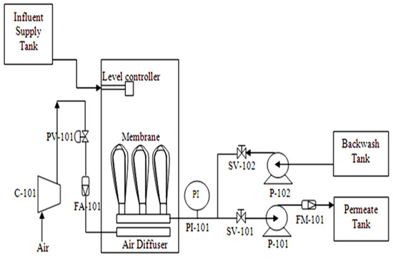
Figure 1.
Schematic diagram of the submerged MBR (SMBR) system.

Table 1.
List of instruments in the pilot plant.
The total of 4000 data for each parameter were collected from the experiment, including airflow (SLPM), permeate pump (voltage), transmembrane pressure (mbar), and permeate flux (L m−2 h−1). Steps input with a random magnitude were excited for the suction pump between 0 to 3 and for the TMP between 0 to 270 mbar to obtain the dynamic behavior of the filtration process. The setting for the permeate-to-relaxation period is maintained at 120 s permeate and 30 s relaxation, with continuous aeration airflow. The airflow was set around six to eight standard liters per minute (SLPM) during filtration to maintain the high intensity of bubble flow in order to clean the membrane surface. Figure 2 shows the SMBR filtration dataset, including permeate pump voltage and TMP as the inputs and permeate flux as an output. The analysis of required data was carried out by using MATLAB R2015a and Design-Expert version 12.0.
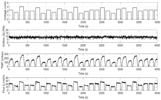
Figure 2.
Dataset from the SMBR filtration experiment.
2.2. Experimental Analyses
The performance of the filtration process is measured based on permeate flux as follows:
where is the permeate flux in (), is the volume flow rate in liters, is the membrane surface area (), and is the time ().
2.3. Simulation Modelling
2.3.1. Artificial Neural Network
The schematic structure of the FFNN is used in the present study for predicting the permeate flux of POME during membrane filtration processes, as shown in Figure 3. The input variables are transmembrane pressure and permeate pump voltage. The output variable is the permeate flux of POME. It was reported in an earlier work [36] that a network with one hidden layer and a hyperbolic tangent sigmoid (tansig) function is commonly used for forecasting in practice. In this work, one hidden layer with a tansig transfer function was considered. For the simulation process, a linear (purelin) function for the output was selected to produce a continuous output. The FFNN used in this study is based on the following equation:
where is the prediction output. is the function of the network is the input vector. and represent the network connection layer weights and biases, respectively.
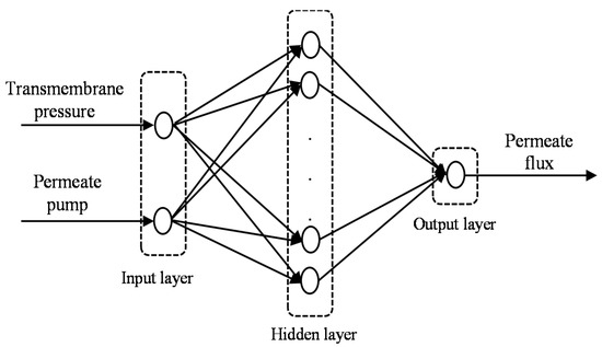
Figure 3.
Schematic structure for FFNN.
In this work, data normalization and data division were performed prior to the development of the neural network model. Since the input data for the SMBR system involved different magnitudes and scales, the dataset is scaled in the range of 0 to 1. This is to prevent the large original input data from dominating the solution. In addition, it prevents numerical difficulties during the calculation [37]. Equation (3) is the formula for normalization [14].
where is the scale value, is the th actual value of data, is the maximum value of data, and is the minimum value of data.
In order to investigate the feasibility of the predictive model, a combination of holdout validation and K-fold cross validation were applied. For holdout validation, all the data were randomly separated into the training dataset (Ttraining) and testing dataset (Ttest). The training dataset is used for training and evaluation of the network, while the testing dataset is employed to test the performance of the network. The dataset is divided into 60% and 40% for training and testing, respectively.
K-fold cross validation is preferable for a large dataset and is chosen in this work. In this study, three-fold cross validation is used. To tune the network parameters, the training dataset is divided into a learning dataset (Tlearning) and validation dataset (Tvalidation). Two thirds of the learning dataset (Tlearning) are the set of patterns that are used to actually train the network. The network performance is evaluated using the validation dataset (Tvalidation), which is the remaining one-third of the pattern in the training data. The procedure was repeated three times, each time using a different fold of the observations into the learning dataset and validation dataset. Then, the average of MSECV was calculated. For the conventional method, the network parameters with a minimum validation error are selected. On the other hand, for the proposed method (FFNN-RSM), the optimal value of network parameters suggested by RSM were used. The network then finally tested on the testing dataset to yield an unbiased estimate of the performance of the network on the unseen dataset.
2.3.2. Network Parameters
The network parameter is one of the main factors in achieving a good performance of a model, including FFNN model structure. Finding the best network parameters is a critical task, and appropriate ranges should be chosen. For conventional-based FFNN, the training process considers numerical factors including the number of neurons, the learning rate, the number of epochs, and the momentum coefficient training parameters. In addition to the numerical factors, the categorical factors such as training function are also considered in this paper for the better performance of model prediction.
The training functions used in this case are Levenberg–Marquardt (lm) and gradient descent with momentum (gdm). The lm training function provides great abilities such as a fast training function, a non-linear regression with a low mean square error (MSE), and memory reduction features [38,39], while the gdm has advantages such as avoiding local minima, speeding up learning, and stabilizing convergence [40]. The gdm training function depends mainly on two parameters of training: the learning rate and momentum parameters.
The former parameter aims to find the minimum weight space. Too high of a learning rate will lead to an increase in the magnitude of the oscillations for MSE, while too low of a learning rate causes smaller steps to be taken in the weight space. In this case, the capability of the network to escape from the local minima in the error surface becomes lower due to a low learning rate. The latter parameter defines the amount of momentum, where a low momentum causes less of a sensitivity of the network to the local gradient, while a high momentum causes a divergence of adaptation, which yields unusable weights. Moreover, it was found in works presented in [40,41,42] that the optimal values of the learning rate and momentum provide smooth behavior and speed up the convergence. The works also claimed that overly low values of the learning rate and momentum slowed down the converging process, while overly high values of the learning rate and momentum might lead to network instability and training divergence.
The number of neurons in the hidden layer plays a decisive role in the network performance, both for the gdm and lm training functions. For FFNN in particular, a small number of hidden neurons will cause less of an adaption in the simulation modelling. However, too big of a number of hidden neurons will cause a low ability of neural network learning, which yields system memory errors [35,40]. There is no systematic method for determining the structure (number of hidden neurons) of the network, mostly by the trial-and-error method. To achieve an accurate neural network approximation, there is an upper bound for the number of hidden neurons, as proposed by [43], which is given in Equation (4):
where is the number of hidden neurons and is the number of inputs.
To avoid an over-fitting problem in the training data, the work in [44] proposed a relationship between the number of samples of the training data and the number of hidden neurons, given in Equation (5):
where is the number of samples of the training data.
Finally, the number of epochs was selected. The number of epochs or training cycles is important to determine network models. In process modelling, a small number of epochs limits the ability of the network, while too many epochs can lead to an overtraining of the network and increase the error [35,40,45]. To train the FFNN model using different training functions (BR, LM, and GD), the maximum setting of the number of epochs is 1000 [38].
For a conventional-based FFNN, to search for optimal conditions, networks were trained under a wide range of parameter settings based on the trial-and-error method. The number of neurons in the hidden layer, the learning rate, the momentum, the number of epochs, and the training function are considered in building an optimum network structure. The optimization was carried out by applying holdout validation and K-fold cross validation on training the datasets. The training dataset was divided into two subsets in order to train the network (Tlearning) and to validate the network (Tvalidation). Mean squared error cross validation (MSECV) is used to estimate the training network. The selection of corresponding FFNN parameters is based on the lowest MSECV for each parameter, which is then used for the testing dataset to verify the reliability of the network models.
The following network parameters were chosen for FFNN optimization: the number of neurons in the hidden layer, the learning rate, the momentum, the epoch number, and the training function. The range of network parameters for FFNN training, both for conventional (lm and gdm) models and the proposed (RSM) model, is shown in Table 2.
Table 2.
The range of ANN training parameters for conventional and RSM models.
2.3.3. Proposed FFNN-RSM Training Method
This section describes the proposed RSM-based FFNN (FFNN-RSM) optimization method. A complete description of the process behavior requires a quadratic or higher order polynomial model. With the use of the least square method, the quadratic models are established to describe the dynamic behavior of the process. The quadratic type of model is usually sufficient for industrial applications and, hence, is used in this work for the modelling of the permeate flux for the POME industry. For k factors, the following quadratic model is utilized and given in Equation (6).
where is the predicted response or dependent variable, are the independent variables, and are the constants. The term is the intercept term, is the linear term, are the squared terms, and is the interaction term between the variables. The input is called a factor, and the output is known as a response.
In this case, there are five factors which consider four numerical factors (number of neurons, learning rate, momentum, and number of epoch) and one categorical factor (training function); therefore, k = 4 was set, which is involved for the numeric factor only. The lowest and the highest levels of variables are coded as −1 and +1, respectively, and are given in Table 2, including the axial star points of (−α and +α), where α is the distance of the axial points from the center and makes the design rotatable. In this study, the α value was fixed at 1 (face centered). The total number of experimental combinations should be conducted based on the concept of central composite design (CCD) by applying Equation (7).
where is the number of independent variables (numerical factors) and is the number of experiments repeated at the center point. Then, is stated as the factorial point, while is stated as an axial point. In this case, and . Since this study involves one categoric factor with two levels (trainlm and traingdm), the number of experiments repeated at the factorial point, axial point, and center point are doubled . Therefore, the total number of runs needed is 60.
A matrix of 60 experiments with four numerical factors and one categorical factor was generated using the software package Design-Expert version 12.0. A total of 12 center points were used to determine the experimental error and reproducibility of the data. Table 3 shows the complete design matrix of the experiments performed and the obtained results of the MSECV. The responses were used to develop an empirical model for the permeate flux of POME. Analysis of variance (ANOVA) at a 5% level of significance, using the Fisher F-test, was used in determining the experimental design, interpretations, and analyses of the training data. An arithmetical method that sorts out the components of a given variation in a set of data and provides a significance test is called the F-test. The predicted response is transformed so that the distribution of the response variable is closer to the normal distribution. The Box-Cox plot is applied to improve model fitting. The transformations used are and , which respectively represent the inverse, natural log, square root, and no transformation functions [35].
Table 3.
MSECV results obtained by various conditions of network parameters using CCD.
The detailed methodology of the development of the proposed FFNN-RSM is depicted in Figure 4.
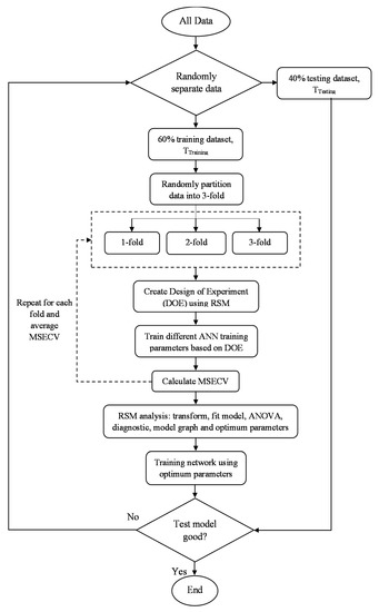
Figure 4.
FFNN-RSM training parameters methodology.
The proposed framework of FFNN-RSM can be described as the following steps:
- Divide all datasets into training datasets (Ttraining) and testing datasets (Ttest);
- Subdivide Ttraining into threefold: 2/3-fold data used to train the network (Tlearning) and 1/3-fold data used to validate the network (Tvalidation);
- Create DoE settings based on RSM;
- Train different network parameters on Tlearning and evaluate its performance on Tvalidation;
- Repeat step (4) for each fold and calculate the average MSECV;e.g., for no. of neuron = 1,[(MSECVfold-1 + MSECVfold-2 + MSECVfold-3)/3] = average MSECVneuron-1;
- Iteratively determine the network parameters by changing different network parameters based on the DoE settings;
- Analyze the DoE data using RSM and select the best neural network parameters;
- Retrain these network parameters on Ttraining;
- Test for the generalization ability using Ttest;
- Compare to determine if it meets the criteria. If not, return to step (1).
2.4. Performance Evaluation
The performance evaluation of the model development is measured using the correlation coefficient ® and mean square error (MSE), as given in Equations (8) and (9):
where , , and denote the i-th independent variable, i-th dependent variable, the mean of dependent variables, and the mean of dependent variables, respectively. The independent and dependent variables are measured by the permeate flux and predicted permeate flux of POME, respectively. Thus, the correlation coefficient was used to assess the strength of the relationship between the inputs (permeate pump and TMP) and the permeate flux output. The MSE value near zero (0) and the R value near one (1) indicate the high accuracy of the prediction model.
3. Results and Discussions
This section is divided into three parts. In the first part, the results of conventional-based FFNN training in selecting neural network parameters are described. The RSM-based FFNN training (FFNN-RSM) results are presented in the second part. All data were normalized. Holdout validation and K-fold cross validation were used to ensure the robustness of the network parameters and to avoid overtraining. Finally, the model validations for permeate flux using optimal parameters from both techniques (conventional FFNN and FFNN-RSM) are presented and discussed. The accuracy of the FFNN models was measured using training and testing regressions.
3.1. Conventional-Based FFNN Training
This section discusses the selection of the optimum number of training parameters for the conventional FFNN. The training parameters include the number of neurons, the learning rate, the momentum coefficient, and the number of epochs. Figure 5 shows the MSECV with a varying number of neurons for FFNN-lm and FFNN-gdm. The determination of the optimum number of network parameters is based on the lowest MSECV value. The number of neurons determines the number of connections between inputs and outputs and may vary depending on specific case studies. If too many neurons are used, the FFNN becomes over-trained, causing it to memorize the training data, which affects finding the best prediction model [30,35,45,46]. In this case, the number of neurons is varied from 1 to 30, which required 30 runs. It can be seen that the optimum number of neurons was obtained at 29 and 8 for FFNN-lm and FFNN-gdm, respectively, with the lowest MSECV values of 0.0238 and 0.0533 for FFNN-lm and FFNN-gdm, respectively. The MSECV values presented by FFNN-gdm tend to fluctuate as the number of neurons varies compared with the FFNN-lm, which is more consistent, as shown in Figure 5.
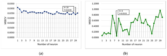
Figure 5.
MSECV with a varying number of neurons for (a) FFNN-lm and (b) FFNN-gdm.
Figure 6 and Figure 7 present the MSECV with varying values of learning rate and momentum, respectively. In this case, both the learning rate and momentum were trained with values set at 0.1 to 1, with 10 runs required for each parameter. As depicted in Figure 6a, it was found that the learning rates of 0.3 (MSECV = 0.0238), 0.5 (MSECV = 0.0239), and 0.7 (MSECV = 0.0232) would probably produce good results for FFNN-lm. However, the learning rates for conventional-based FFNN were obtained at 0.7 and 0.2 for lm and gdm, respectively, which gave the lowest MSECV of 0.0232 and 0.3403 for lm and gdm, respectively.
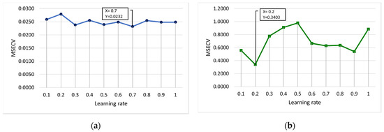
Figure 6.
MSECV with varying values of the learning rate for (a) FFNN-lm and (b) FFNN-gdm.
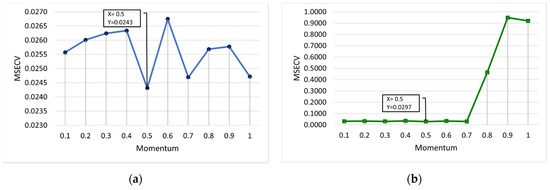
Figure 7.
MSECV with varying values of momentum for (a) FFNN-lm and (b) FFNN-gdm.
Figure 7 shows the optimum values of the momentum coefficient for FFNN-lm and FFNN-gdm. Both lm and gdm provide same value of momentum at 0.5. At this momentum value, the lowest MSECVs of 0.0243 and 0.0297 were obtained for lm and gdm, respectively. It can be observed in Figure 7b that the MSECV values of FFNN-gdm are slightly consistent at minimum values for the number of momentums at 0.1 until 0.7, with MSECVs of 0.0313, 0.0334, 0.0308, 0.0351, 0.0297, 0.0334, and 0.0303, respectively. Then, the increase in the momentum values for FFNN-gdm showed a sudden increment in MSECV to almost 1.
Figure 8 shows the MSECV with varying numbers of epochs for FFNN-lm and FFNN-gdm. In this case, the number of epochs is varied from 100 to 1000, and 10 runs are required. As illustrated in Figure 8b, it was found that the number of epochs that may produce a good outcome is 600 and 1000 with MSECVs of 0.0310 and 0.0302, respectively. Therefore, the optimum values of each epoch are obtained at 300 for lm, and 1000 for gdm was selected, which gave the lowest MSECV values of 0.0234 and 0.0302, respectively.
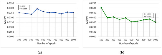
Figure 8.
MSECV with varying numbers of epochs for (a) FFNN-lm and (b) FFNN-gdm.
Table 6 summarizes the optimal values of the training parameters obtained for the conventional-based FFNN (FFNN-lm and FFNN-gdm).
3.2. RSM-Based FFNN Training
This section presents the optimum number of training parameters obtained using the RSM-based FFNN training. In this case, the proposed FFNN-RSM method utilized a face-central composite design (CCD) of four numerical factors (number of neurons, learning rate, momentum, and number of epochs) and one categorical factor (training function), and a two-level (trainlm and traingdm) design matrix was selected. The experimental design matrix is shown in Table 3. There are 60 sets of conditions (run) which consist of 32 factorial points, 16 axial points, and 12 center points. The different conditions of the neural network parameters were designed and trained to model the best MSE performance on the Tvalidation dataset using the Design-Expert software.
In this work, the quadratic model was chosen to yield the correlation between the neural network effective factors (input) and the response of MSECV (output). Using the Box-Cox method, the MSECV response is transformed to a natural log (ln(MSECV)), with α equal to 1. The transformation will make the distribution of the response closer to the normal distribution and improve the fit of the model to the data [35]. The quadratic model in terms of coded factors for ln(MSECV) of the FFNN-RSM model is given in Equation (10):
where the A, B, C, D, and E parameters are the code values of the number of neurons, the learning rate, the momentum, the number of epochs, and the training function, respectively, as presented in Table 3. Equation (10) is used for predictions of the response at a given level of each factor. The coded equation is useful for identifying the relative impact of the factors by comparing the factor coefficients. Negative and positive values of the coefficients represent antagonistic and synergistic effects of each model term, respectively. The positive value causes an increase in the response, while the negative value represents a decrease in the response. The values of the coefficients are relatively low, due to the low values of the MSECVs responses of the system [47].
The accuracy of the RSM model is determined using ANOVA. The ANOVA contains the set of evaluation terms such as the coefficient of determination (R2), adjusted R2, predicted R2, adequate precision, F-value, and p-value, which are used to explain the significance of the model. Table 4 illustrates the ANOVA for the response surface of the quadratic model. The statistical test factor, F-value, was used to evaluate the significance of the model at the 95% confidence level [30]. The p-value serves as a tool to ensure the importance of each coefficient at a specified level of significance. Generally, a p-value of less than 0.050 showed the most significance and contributes largely toward the response. The smaller the p-value, the more significant the corresponding coefficient. Other values that are greater than 0.050 are less significant.
Table 4.
Analysis of variance (ANOVA) for the response surface of the quadratic model.
Table 4 presents the ANOVA for the response surface of the quadratic model. The highest F-value (15.35) had a p-value lower than 0.0001, confirming that the model is statistically significant. The lack-of-fit test for the model showed insignificance with an F-value of 0.7680 and a p-value of 0.7262. This indicates that the model adequately fitted the experimental data. The value of R2 of 0.8794 showed a good correlation between the predicted and actual values of the responses. The value of predicted R2 of 0.7183 is in reasonable agreement with the adjusted R2 of 0.8221, also indicating the significance of the model [33]. The closer the R2 value is to unity, the better the model will be, as it will yield predicted values closer to the actual values. The adequate precision measures the signal-to-noise ratio, and in this analysis, (14.8721) indicates an adequate signal. A ratio greater than 4 is desirable. Thus, the model can be used to navigate the design space [30].
The p-values less than 0.050 (A, B, C, E, AE, BE, CE) indicate significant effects of the prediction process. The statistical analysis showed that the first order effect or linear term of training functions (E) is the most significant term in the ln(MSECV) response, followed by the number of neurons, the momentum, and the learning rate. The number of epochs depicted a less significant effect on the response, with an F-value = 0.0464 and a p-value = 0.8305. In addition, the p-values of AB, AC, AD, BC, BD, CD, DE, A2, B2, C2, and D2 are greater than 0.050 and, hence, less important in the ANN training process.
Figure 9 shows the plot of response (ln(MSECV)) and the interaction factors (number of neurons, learning rate, momentum, and number of epoch) obtained from the model graph of the Design-Expert version 12.0 software. Figure 9a shows the interaction plot of the number of neurons versus the ln(MSECV) of the training function with the other interaction factors, which are constant at their midpoints. In Figure 9a, the different shapes of curves depend on the type of training function (E). It can be observed that, with an increased number of neurons (from 1 to 30) and with traingdm as a training function, the ln(MSECV) increases up to 0.7. This indicates that too many hidden neurons yield more flexibility for the weight adjustment and, hence, a better learning process, particularly with noise present in the system.
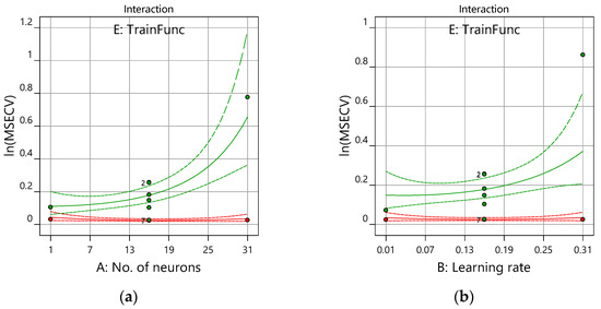
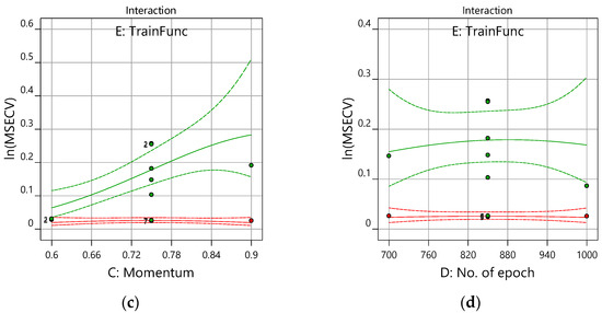
Figure 9.
Interaction plot for the ANN training parameters of ln(MSECV) versus the (a) number of neurons, (b) learning rate, (c) momentum, and (d) number of epochs. trainlm—red; traingdm—green.
Almost similar trends can be seen for an increased learning rate and momentum. However, by increasing the number of epochs (i.e., from 700 to 1000), it showed less of an effect on the ln(MSECV) response from the curves depicted in Figure 9d. These findings confirmed the statistical results obtained in Table 4—the number of neurons, the learning rate, and the momentum were significant variables for ln(MSECV), while the epoch number is not trivial. There is very little change or interaction shown by ln(MSECV) for FFNN-lm compared with ln(MSECV) for FFNN-gdm. This is because the MSECV value produced by FFNN-lm is too small, since Levenberg–Marquart (lm) has advantages such as the fastest training function and a good function fitting (non-linear regression) with a lower mean square error (MSE).
The comparisons of the actual and predicted ln(MSECV) responses based on 60 runs of various conditions of the network parameters using CCD are given in Table 5. From Table 5, the overall actual values of ln(MSECV) matched with the predicted values of ln(MSECV). This indicates that the quadratic model in Equation (10) can be established to identify the relationship between the MSECV and the network parameters.
Table 5.
Comparisons of the actual and predicted ln(MSECV) by various conditions of network parameters.
Figure 10a,b show the perturbation plots for the lm and gdm training functions, respectively. The perturbation graph is required to see how the response changes to the changes of its factor from the reference point, with other factors held at constant reference values. In this case, the reference points default at the middle of the design space (the coded zero level of each factor). Figure 10a presents good interaction variables of the ln(MSECV) response with FFNN-lm. At the center point, factors A (number of neurons), B (learning rate), and C (momentum) produce a relatively higher effect for changes in the reference point, while only a small effect is produced by factor D (number of epoch).
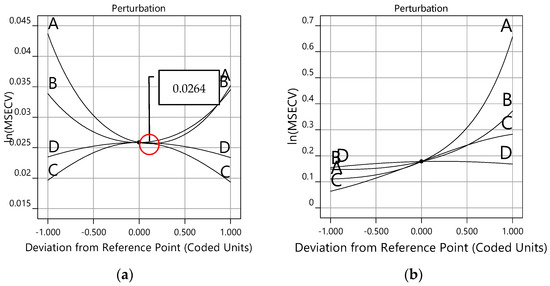
Figure 10.
Perturbation plot for training functions, (a) trainlm and (b) traingdm.
Notice that the optimum values of ln(MSECV) for the network parameters (A, B, C, and D) can be found at 0.0000 (coded value), as shown in Figure 10a for the lm training function and in Figure 10b for the gdm training function. In this case, the optimum values for A, B, C, and D are, respectively, 16, 0.16, 0.75, and 850, as presented in Table 6. It can be observed that both Figure 9 and Figure 10 present similar plots of ln(MSECV), but the former plot represents the interaction graph which uses the actual value of the variables, while the latter represents the perturbation graph which uses coded values. Both graphs describe the relationship of the network parameters. As shown in Table 6, the best network parameters obtained from the conventional and proposed methods are presented for all network parameters. Therefore, the optimum values suggested by RSM were as follows: number of neurons = 16, learning rate = 0.16, momentum = 0.75, and number of epochs = 850, and trainlm has been selected as a training function. The best network parameters for FFNN-lm had minimum MSECVs when the number of neurons, the learning rate, the momentum, the number of epoch and the training function were 29, 0.7, 0.5, 300, and trainlm, respectively. Furthermore, the minimum MSECV was obtained by employing the following optimum condition for the FFNN-gdm network parameters: number of neurons = 8, learning rate = 0.2, momentum = 0.5, number of epochs = 1000, and training function = traingdm. These optimum values were applied for predicting the permeate flux of POME.
Table 6.
The best network parameters for the FFNN-lm, FFNN-gdm, and FFNN-RSM models.
It may be concluded that too few hidden neurons limit the ability of the FFNN-lm to model the process well. Too many hidden neurons cause over-fitting and increase the computation time. The learning rate determines the time needed to find the minimum in the weight space. Too small of a learning rate leads to smaller steps being taken in the weight space, a slow learning process, and the network being less capable of escaping from the local minima in the error surface. Too high of a learning rate leads to an increased magnitude of the oscillations for the mean square error and a resulting slow convergence to the lower error state. Moreover, if the momentum is too small, then it will lengthen the learning process.
3.3. Model Validation
Figure 11a shows the training results for the permeate flux outputs for the FFNN-lm, FFNN-gdm, and FFNN-RSM models. These models are plotted based on the best ANN training parameters. From Figure 11a, it can be observed that the predicted datasets for all ANN models have similar trends to the actual or measured datasets. The permeate flux models for FFNN-lm have a slightly different shape with FFNN-gdm, but it is almost similar to FFNN-RSM. This is because FFNN-RSM also uses the trainlm training function as a model setting.
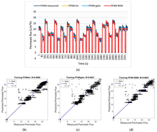
Figure 11.
(a) Permeate flux for FFNN−measured, FFNN−lm, FFNN−gdm, and FFNN−RSM models. Comparison of the measured and predicted permeate flux of POME between (b) FFNN−lm, (c) FFNN−gdm, and (d) FFNN−RSM for the training dataset.
The dotted lines in Figure 11b–d represent the (perfect result—outputs = targets), and the solid line represents the best fit linear regression between the target and the output for FFNN-lm, FFNN-gdm, and FFNN-RSM using training data, respectively. Moreover, the FFNN model trained with trainlm using the conventional method (FFNN-lm) showed the highest accuracy with the correlation coefficient, with the R and MSE at 0.9888 and 0.0223, respectively, followed by FFNN-RSM (0.9881 and 0.0237) and FFNN-gdm, which were 0.9851 and 0.0296, respectively (refer to Figure 11b–d). In terms of accuracy, FFNN-lm and FFNN-RSM are comparable.
The training model was then validated using the testing dataset, and good agreement with the actual dataset was achieved, as shown in Figure 12a–d. Figure 12a shows the plot of FFNN-lm, FFNN-gdm, and FFNN-RSM permeate flux models for the SMBR filtration system during testing datasets. From Figure 12b–d, it can be seen that all the models demonstrated good prediction, with a slightly higher performance of accuracy for FFNN-lm, followed by FFNN-RSM and FFNN-gdm. The FFNN-lm model resulted in 0.9873 and 0.0253 for R and MSE, respectively. The R and MSE for FFNN-RSM are, respectively, 0.9866 and 0.0265, while the performance of the FFNN-gdm testing model was 0.9847 and 0.0303 for the R and FFNN-RSM models during the training and testing datasets.
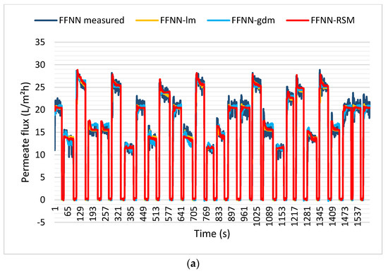
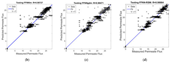
Figure 12.
(a) Permeate flux for FFNN−measured, FFNN−lm, FFNN−gdm, and FFNN−RSM models. Comparison of the measured and predicted permeate flux of POME between (b) FFNN−lm, (c) FFNN−gdm, and (d) FFNN−RSM for the testing dataset.
From Table 7, it was found that all FFNN models produced comparable results for both the training and testing accuracy performance. Nevertheless, in terms of the amount of repetition and training time of the proposed method and the conventional method, the proposed method (FFNN-RSM) only required 60 runs in 233 s (00:03:53) to determine the optimal value of ANN training parameters for the FFNN model. The conventional method required 60 runs for each model (a total of 120 runs), with a total training time of 543 s for both models, which is 151 s (00:02:31.02) for FFNN-lm and 392 s (00:09:03.07) for FFNN-gdm. It is proven that the RSM technique depicted a high performance and the fastest model training technique when compared with the conventional method.
Table 7.
Overall performance accuracy of the FFNN-lm, FFNN-gdm, and FFNN-RSM models for the SMBR filtration system.
Despite the well-known advantage of the neural network in predicting larger datasets, these results show that the combined FFNN-RSM model can predict well and provide a comparable result in relation to the conventional method in this case. The FFNN-RSM shows a robust generalization ability with a small generalization error. With a smaller number of repetitions, RSM is also effective in avoiding monotonous tasks, where several different network parameters must be constructed, trained, and tested. Moreover, RSM has an ability to analyze the significant parameters and interaction effects of the parameters that affect the output response, which is the MSECV of the model. Hence, RSM is observed as satisfying the requirement for the optimization of ANN training parameters in order to obtain a good prediction model.
4. Conclusions
The FFNN model has been successfully developed for the permeate flux of POME during the submerged membrane bioreactor (SMBR) filtration process. The combined FFNN-RSM model has been developed to determine the network parameters, and it has been compared with conventional trial-and-error models (FFNN-lm and FFNN-gdm). The model validation results showed that good validity of the training and testing models was obtained for all models. The simulation results showed the comparable performance accuracy of the FFNN-RSM model in relation to both conventional FFNN models. The optimization of the ANN training parameters for the FFNN-RSM models shows an improved training time and number of repetitions—by about 57% and 50%, respectively—compared to the conventional FFNN model. The benefit of RSM is due to the application of the design of experiment (DoE), which requires less repetition of the training process but can provide a huge sum of information. In this work, the RSM successfully determines the best network parameters for the FFNN model. Moreover, it learned the significance and the relationship between the ANN training parameters and the MSECV.
The FFNN models (FFNN-lm, FFNN-gdm, and FFNN-RSM) demonstrated good and comparable prediction models, with a slightly higher performance of accuracy for FFNN-lm (0.9873), followed by FFNN-RSM (0.9866) and FFNN-gdm (0.9847). However, FFNN-RSM only required 60 runs in 233 s to determine the optimal value of ANN training parameters. Meanwhile, the conventional method required 60 runs for each model (a total of 120 runs), with a total training time of 543 s for both models, which is 151 s for FFNN-lm and 392 s for FFNN-gdm. The FFNN-RSM technique showed an improvement over the conventional FFNN model in terms of the number of repetitions, the training time, and the estimation capabilities. This significant improvement can be later used in control system development to improve membrane operation.
Author Contributions
Data curation, S.I.; methodology, S.I.; validation, S.I.; software, S.I.; investigation, S.I.; supervision, N.A.W.; writing—original draft preparation, S.I.; writing—review and editing, N.A.W. All authors have read and agreed to the published version of the manuscript.
Funding
This research was supported/funded by Universiti Teknologi Malaysia High Impact University Grant (UTMHI): 08G74 and Ministry of Education (MOE) PRGS: R.J130000.7851.4L702.
Institutional Review Board Statement
Not applicable.
Informed Consent Statement
Not applicable.
Data Availability Statement
Not applicable.
Acknowledgments
This work was supported financially by the Universiti Teknologi Malaysia High Impact University Grant (UTMHI) vote Q.J130000.2451.08G74 and was supported in part by the Ministry of Higher Education under the Prototype Research Grant Scheme (PRGS/1/2019/TK04/UTM/02/3).
Conflicts of Interest
The authors declare no conflict of interest.
Abbreviations
List of abbreviations:
| ANN | - | artificial neural network |
| ANOVA | - | analysis of variance |
| BOD | - | biochemical oxygen demand |
| BR | - | Bayesian regulation |
| CCD | - | central composite design |
| DE | - | differential evaluation |
| DoE | - | design of experiment |
| FFNN | - | feed-forward neural network |
| FFNN-gdm | - | conventional gradient descent with momentum-based FFNN |
| FFNN-lm | - | conventional Levenberg–Marquardt-based FFNN |
| FFNN-RSM | - | proposed RSM-based FFNN |
| GA | - | genetic algorithm |
| GD | - | gradient descent |
| gdm | - | gradient descent with momentum |
| HP | - | host power |
| kDa | - | kilo Daltons |
| L | - | liter |
| L m−2 h−1 | - | liter per meter square hour |
| L min−1 | - | liter per minute |
| lm | - | Levenberg–Marquardt |
| ln(MSECV) | - | natural log mean square error cross validation |
| mbar | - | millibar |
| mg L−1 | - | milligram per liter |
| MSE | - | mean square error |
| MSECV | - | mean square error cross validation |
| N/A | - | not available |
| NI USB | - | national instruments universal serial bus |
| OVAT | - | one-variable-at-time |
| PES | - | polyethersulfone |
| POME | - | palm oil mill effluent |
| PSO | - | particle swarm optimization |
| purelin | - | linear function |
| R | - | correlation coefficient |
| R2 | - | coefficient of determination |
| RSM | - | response surface methodology |
| SLPM | - | standard liter per minute |
| SMBR | - | submerged membrane bioreactor |
| tansig | - | hyperbolic tangent sigmoid |
| TMP | - | transmembrane pressure |
| traingdm | - | gradient descent with momentum training function |
| trainlm | - | Levenberg–Marquardt training function |
| Volt | - | voltage |
References
- Alkhatib, M.F.; Mamun, A.A.; Akbar, I. Application of response surface methodology (RSM) for optimization of color removal from POME by granular activated carbon. Int. J. Environ. Sci. Technol. 2015, 12, 1295–1302. [Google Scholar] [CrossRef]
- Wah, W.P.; Nik Meriam, S.; Nachiappan, M.; Varadaraj, B. Pre-treatment and membrane ultrafiltration using treated palm oil mill effluent (POME). Songklanakarin J. Sci. Technol. 2002, 24, 891–898. [Google Scholar]
- Cassano, A.; Basile, A. Membranes for industrial microfiltration and ultrafiltration. In Advanced Membrane Science and Technology for Sustainable Energy and Environmental Applications, 1st ed.; Basile, A., Nunes, S.P., Eds.; Elsevier: Amsterdam, The Netherlands, 2011; pp. 647–679. [Google Scholar]
- Mohd Syahmi Hafizi, G.; Haan, T.Y.; Lun, A.W.; Abdul Wahab Mohammad Rahmat, N.; Khairul Muis, M. Fouling assessment of tertiary palm oil mill effluent (POME) membrane treatment for water reclamation. J. Water Reuse Desalin. 2018, 8, 412–423. [Google Scholar]
- Leiknes, T. Wastewater treatment by membrane bioreactors. In Membrane Operations: Innovative Separations and Transformations; Drioli, E., Giorno, L., Eds.; WILEY-VCH Verlag GmbH & Co. KGaA: Rende, Italy, 2009; pp. 374–391. [Google Scholar]
- Lin, H.; Gao, W.; Meng, F.; Liao, B.Q.; Leung, K.T.; Zhao, L.; Chen, J.; Hong, H. Membrane bioreactors for industrial wastewater treatment: A critical review. Crit. Rev. Environ. Sci. Technol. 2012, 42, 677–740. [Google Scholar] [CrossRef]
- Janus, T. Modelling and Simulation of Membrane Bioreactors for Wastewater Treatment. Ph.D. Thesis, De Montfort University, Leicester, UK, 2013. [Google Scholar]
- Stuckey, D.C. Recent developments in anaerobic membrane reactors. Bioresour. Technol. 2012, 122, 137–148. [Google Scholar] [CrossRef] [PubMed]
- Yusuf, Z.; Wahab, N.A.; Sudin, S. Soft computing techniques in modelling of membrane filtration system: A review. Desalin. Water Treat. 2019, 161, 144–155. [Google Scholar] [CrossRef]
- Farkas, I.; Reményi, P.; Biró, A. A neural network topology for modelling grain drying. Comput. Electron. Agric. 2000, 26, 147–158. [Google Scholar] [CrossRef]
- Pakravan, P.; Akhbari, A.; Moradi, H.; Azandaryani, A.H.; Mansouri, A.M.; Safari, M. Process modeling and evaluation of petroleum refinery wastewater treatment through response surface methodology and artificial neural network in a photocatalytic reactor using poly ethyleneimine (PEI)/titania (TiO2) multilayer film on quartz tube. Appl. Petrochem. Res. 2015, 5, 47–59. [Google Scholar] [CrossRef]
- Kasiviswanathan, K.S.; Agarwal, A. Radial basis function artificial neural network: Spread selection. Int. J. Adv. Comput. Sci. 2012, 2, 394–398. [Google Scholar]
- Razmi-Rad, E.; Ghanbarzadeh, B.; Mousavi, S.M.; Emam-Djomeh, Z.; Khazaei, J. Prediction of rheological properties of Iranian bread dough from chemical composition of wheat flour by using artificial neural networks. J. Food Eng. 2007, 81, 728–734. [Google Scholar] [CrossRef]
- Demirbay, B.; Bayram, D.; Uğur, Ş. A Bayesian regularized feed-forward neural network model for conductivity prediction of PS/MWCNT nanocomposite film coatings. Appl. Soft Comput. J. 2020, 96, 106632. [Google Scholar] [CrossRef]
- Fatimah, I.; Mohd Nasir, T.; Wan Abu Bakar, W.A.; Guan, C.C.; Saadiah, S. A novel dengue fever (DF) and dengue haemorrhagic fever (DHF) analysis using artificial neural network (ANN). Comput. Methods Programs Biomed. 2005, 79, 273–281. [Google Scholar]
- Mahfuzah, M.; Mohd Nasir, T.; Zunairah, H.M.; Norizam, S.; Siti Armiza, M.A. The analysis of EEG spectrogram image for brainwave balancing application using ANN. In Proceedings of the 2011 UkSim 13th International Conference on Computer Modelling and Simulation, Cambridge, UK, 30 March–1 April 2011; pp. 64–68. [Google Scholar]
- Mustafa, M.; Nasir Taib, M.; Murat, Z.; Sulaiman, N. Comparison between KNN and ANN classification in brain balancing application via spectrogram image. J. Comput. Sci. Comput. Math. 2012, 2, 17–22. [Google Scholar] [CrossRef]
- Elfghi, F.M. A hybrid statistical approach for modeling and optimization of RON: A comparative study and combined application of response surface methodology (RSM) and artificial neural network (ANN) based on design of experiment (DOE). Chem. Eng. Res. Des. 2016, 113, 264–272. [Google Scholar] [CrossRef]
- Rahmanian, B.; Pakizeh, M.; Mansoori, S.A.A.; Abedini, R. Application of experimental design approach and artificial neural network (ANN) for the determination of potential micellar-enhanced ultrafiltration process. J. Hazard. Mater. 2011, 187, 67–74. [Google Scholar] [CrossRef]
- Taheri-Garavand, A.; Rafiee, S.; Keyhani, A.; Javadikia, P. Modeling of basil leaves drying by GA–ANN. Int. J. Food Eng. 2013, 9, 393–401. [Google Scholar] [CrossRef]
- Curteanu, S.; Leon, F.; Furtuna, R.; Dragoi, E.N.; Curteanu, N.D.; Curteanu, N. Comparison between different methods for developing neural network topology applied to a complex polymerization process. In Proceedings of the 2010 International Joint Conference on Neural Networks (IJCNN), Barcelona, Spain, 18–23 July 2010; pp. 18–23. [Google Scholar]
- Vijayaraghavan, V.; Lau, E.V.; Goyal, A.; Niu, X.; Garg, A.; Gao, L. Design of explicit models for predicting the efficiency of heavy oil-sand detachment process by floatation technology. Meas. J. Int. Meas. Confed. 2019, 137, 122–129. [Google Scholar] [CrossRef]
- Fu, H.; Xu, P.; Huang, G.; Chai, T.; Hou, M.; Gao, P. Effects of aeration parameters on effluent quality and membrane fouling in a submerged membrane bioreactor using Box–Behnken response surface methodology. Desalination 2012, 302, 33–42. [Google Scholar] [CrossRef]
- Ghalekhani, G.R.; Zinatizadeh, A.A.L. Process analysis and optimization of industrial estate wastewater treatment using conventional and compartmentalized membrane bioreactor: A comparative study. Iran. J. Energy Environ. 2014, 5, 101–112. [Google Scholar] [CrossRef][Green Version]
- Siddiqui, M.F.; Singh, L.; Zularisam, A.W.; Sakinah, M. Biofouling mitigation using Piper betle extract in ultrafiltration MBR. Desalin. Water Treat. 2013, 51, 6940–6951. [Google Scholar] [CrossRef]
- Bas, D.; Boyaci, I.H. Modeling and optimization II: Comparison of estimation capabilities of response surface methodology with artificial neural networks in a biochemical reaction. J. Food Eng. 2007, 78, 846–854. [Google Scholar] [CrossRef]
- Deshmukh, S.C.; Senthilnath, J.; Dixit, R.M.; Malik, S.N.; Pandey, R.A.; Vaidya, A.N.; Omkar, S.N.; Mudliar, S.N. Comparison of radial basis function neural network and response surface methodology for predicting performance of biofilter treating toluene. J. Softw. Eng. Appl. 2012, 5, 595–603. [Google Scholar] [CrossRef]
- Desai, K.M.; Survase, S.A.; Saudagar, P.S.; Lele, S.S.; Singhal, R.S. Comparison of artificial neural network (ANN) and response surface methodology (RSM) in fermentation media optimization: Case study of fermentative production of scleroglucan. Biochem. Eng. J. 2008, 41, 266–273. [Google Scholar] [CrossRef]
- Jawad, J.; Hawari, A.H.; Zaidi, S.J. Modeling and sensitivity analysis of the forward osmosis process to predict membrane flux using a novel combination of neural network and response surface methodology techniques. Membranes 2021, 11, 70. [Google Scholar] [CrossRef] [PubMed]
- Nourbakhsh, H.; Emam-Djomeh, Z.; Omid, M.; Mirsaeedghazi, H.; Moini, S. Prediction of red plum juice permeate flux during membrane processing with ANN optimized using RSM. Comput. Electron. Agric. 2014, 102, 1–9. [Google Scholar] [CrossRef]
- Khayet, M.; Cojocaru, C.; Essalhi, M. Artificial neural network modeling and response surface methodology of desalination by reverse osmosis. J. Membr. Sci. 2011, 368, 202–214. [Google Scholar] [CrossRef]
- Ravikumar, R.; Renuka, K.; Sindhu, V.; Malarmathi, K.B. Response surface methodology and artificial neural network for modeling and optimization of distillery spent wash treatment using Phormidium valderianum BDU 140441. Pol. J. Environ. Stud. 2013, 22, 1143–1152. [Google Scholar]
- Sinha, K.; Saha PDas Datta, S. Response surface optimization and artificial neural network modeling of microwave assisted natural dye extraction from pomegranate rind. Ind. Crops Prod. 2012, 37, 408–414. [Google Scholar] [CrossRef]
- Nazghelichi, T.; Aghbashlo, M.; Kianmehr, M.H. Optimization of an artifial neural network topology using couple response surface meethodology and genetic algorithm for fluidized bed drying. Comput. Electron. Agric. 2011, 75, 84–91. [Google Scholar] [CrossRef]
- Aghbashlo, M.; Kianmehr, M.H.; Nazghelichi, T.; Rafiee, S. Optimization of an artificial neural network topology for predicting drying kinetics of carrot cubes using combined response surface and genetic algorithm. Dry. Technol. 2011, 29, 770–779. [Google Scholar] [CrossRef]
- Said, M.; Ba-Abbad, M.; Rozaimah Sheik Abdullah, S.; Wahab Mohammad, A. Artificial neural network (ANN) for optimization of palm oil mill effluent (POME) treatment using reverse osmosis membrane. J. Phys. Conf. Ser. 2018, 1095, 012021. [Google Scholar] [CrossRef]
- Kumar, S. Neural Networks, a Classroom Approach, 2nd ed.; MC Graw-Hill Education: New Dheli, India, 2011. [Google Scholar]
- Keong, K.C.; Mustafa, M.; Mohammad, A.J.; Sulaiman, M.H.; Abdullah, N.R.H. Artificial neural network flood prediction for sungai isap residence. In Proceedings of the 2016 IEEE International Conference on Automatic Control and Intelligent Systems (I2CACIS), Shah Alam, Malaysia, 22 October 2016; pp. 236–241. [Google Scholar]
- Santhosh, A.J.; Tura, A.D.; Jiregna, I.T.; Gemechu, W.F.; Ashok, N.; Ponnusamy, M. Optimization of CNC turning parameters using face centred CCD approach in RSM and ANN-genetic algorithm for AISI 4340 alloy steel. Results Eng. 2021, 11, 100251. [Google Scholar] [CrossRef]
- Winiczenko, R.; Górnicki, K.; Kaleta, A.; Janaszek-Mańkowska, M. Optimisation of ANN topology for predicting the rehydrated apple cubes colour change using RSM and GA. Neural Comput. Appl. 2016, 30, 1795–1809. [Google Scholar] [CrossRef] [PubMed]
- Yousif, J.H.; Kazem, H.A. Case studies in thermal engineering prediction and evaluation of photovoltaic-thermal energy systems production using artificial neural network and experimental dataset. Case Stud. Therm. Eng. 2021, 27, 101297. [Google Scholar] [CrossRef]
- Nayak, K.P.; Padmashree, T.K.; Rao, S.N.; Cholayya, N.U. Artificial neural network for the analysis of electroencephalogram. In Proceedings of the 2006 Fourth International Conference on Intelligent Sensing and Information Processing, Bangalore, India, 15–18 December 2006; pp. 170–173. [Google Scholar]
- Hecht-Nielsen, R. Theory of the backpropagation neural network. In Neural Networks for Perception; Wechsler, H., Ed.; Academic Press: Cambridge, MA, USA, 1992; pp. 65–93. [Google Scholar]
- Rogers, L.L.; Dowla, F.U. Optimization of groundwater remediation using artificial neural networks with parallel solute transport modeling has been successfully applied to a variety of optimization. Water Resour. Res. 1994, 30, 457–481. [Google Scholar] [CrossRef]
- Madadlou, A.; Emam-Djomeh, Z.; Mousavi, M.E.; Ehsani, M.; Javanmard, M.; Sheehan, D. Response surface optimization of an artificial neural network for predicting the size of re-assembled casein micelles. Comput. Electron. Agric. 2009, 68, 216–221. [Google Scholar] [CrossRef]
- Hitsov, I.; Maere, T.; De Sitter, K.; Dotremont, C.; Nopens, I. Modelling approaches in membrane distillation: A critical review. Sep. Purif. Technol. 2015, 142, 48–64. [Google Scholar] [CrossRef]
- Podstawczyk, D.; Witek-Krowiak, A.; Dawiec, A.; Bhatnagar, A. Biosorption of copper(II) ions by flax meal: Empirical modeling and process optimization by response surface methodology (RSM) and artificial neural network (ANN) simulation. Ecol. Eng. 2015, 83, 364–379. [Google Scholar] [CrossRef]


Publisher’s Note: MDPI stays neutral with regard to jurisdictional claims in published maps and institutional affiliations. |
© 2022 by the authors. Licensee MDPI, Basel, Switzerland. This article is an open access article distributed under the terms and conditions of the Creative Commons Attribution (CC BY) license (https://creativecommons.org/licenses/by/4.0/).