
The Role of Soil Structure Interaction in the Fragility Assessment of HP/HT Unburied Subsea Pipelines


Abstract
:1. Introduction
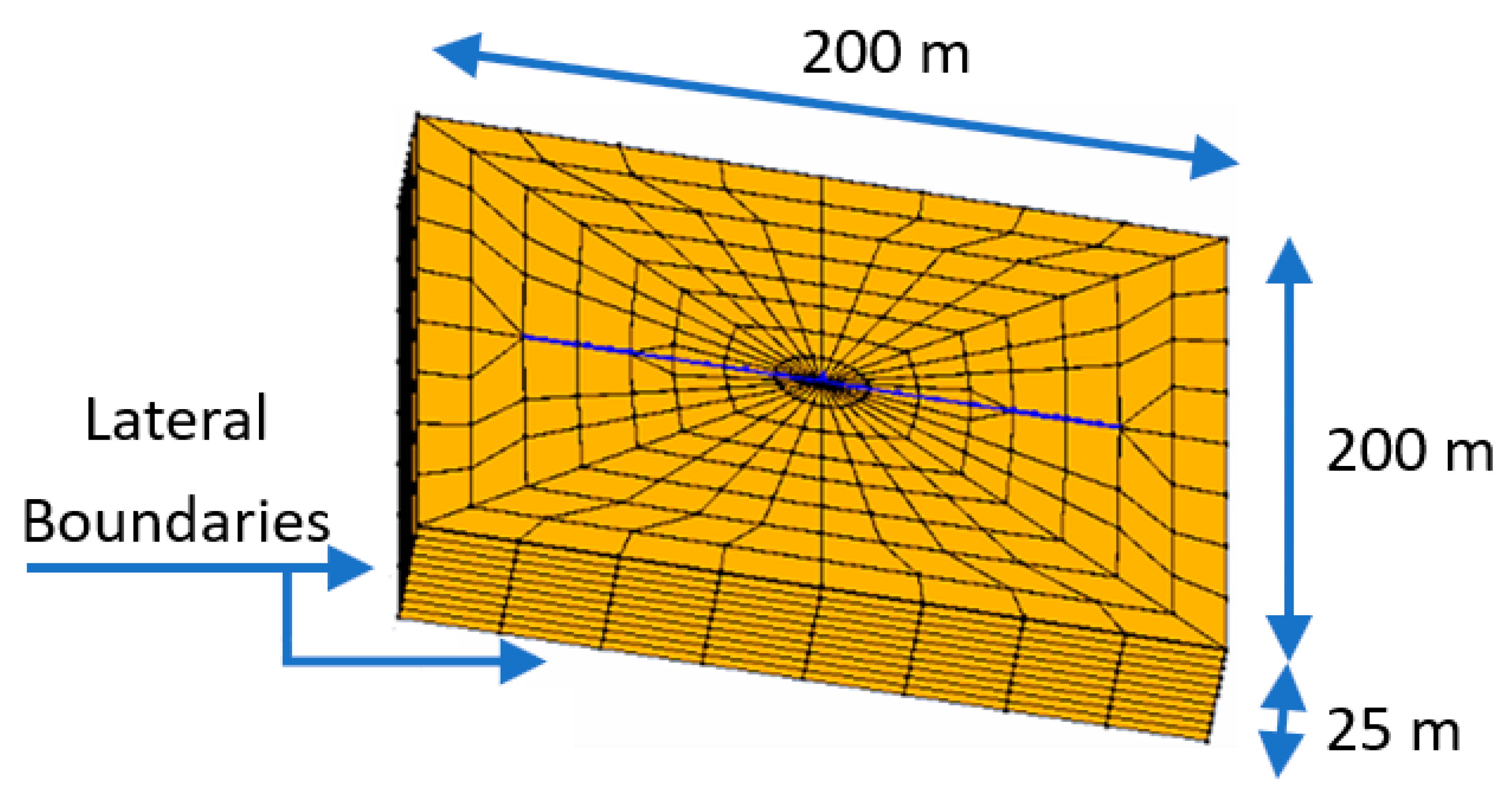
2. Numerical Model
3. Pipeline Failure Criteria
4. Results and Discussion
5. Conclusions
Author Contributions
Funding
Institutional Review Board Statement
Informed Consent Statement
Conflicts of Interest
References
- Yun, H.; Kyriakides, S. On the beam and shell modes of buckling of buried pipelines. Soil Dyn. Earthq. Eng. 1990, 9, 179–193. [Google Scholar] [CrossRef]
- Daiyan, N.; Kenny, S.; Phillips, R.; Popescu, R. Numerical investigation of oblique pipeline/soil interaction in sand. In Proceedings of the 8th International Pipeline Conference, IPC2010-31644, Calgary, AB, Canada, 4 April 2011. [Google Scholar]
- Vazouras, P.; Karamanos, S.A.; Dakoulas, P. Mechanical behavior of buried steel pipes crossing active strike-slip faults. Soil Dyn. Earthq. Eng. 2012, 41, 164–180. [Google Scholar] [CrossRef]
- Vazouras, P.; Dakoulas, P.; Karamanos, S.A. Pipe-soil interaction and pipeline performance under strike-slip fault movements. Soil Dyn. Earthq. Eng. 2015, 72, 48–65. [Google Scholar] [CrossRef]
- Vazouras, P.; Karamanos, S.A.; Dakoulas, P. Finite element analysis of buried steel pipelines under strike-slip fault displacements. Soil Dyn. Earthq. Eng. 2010, 30, 1361–1376. [Google Scholar] [CrossRef]
- Mina, D.; Forcellini, D.; Karampour, H. Analytical fragility curves for assessment of the seismic vulnerability of hp/ht unburied subsea pipelines. Soil Dyn. Earthq. Eng. 2020, 137, 106308. [Google Scholar] [CrossRef]
- Triantafyllaki, A.; Papanastasiou, P.; Loukidis, D. Numerical analysis of the structural response of unburied offshore pipelines crossing active normal and reverse faults. Soil Dyn. Earthq. Eng. 2020, 137, 106296. [Google Scholar] [CrossRef]
- Alrsai, M.; Karampour, H. Propagation buckling of pipe-in-pipe systems, an experimental study. In Proceedings of the Twelfth ISOPE Pacific/Asia Offshore Mechanics Symposium, Old Coast, Australia, 4–7 October 2016. [Google Scholar]
- Binazir, A.; Karampour, H.; Sadowski, A.J.; Gilbert, B.P. Pure bending of pipe-in-pipe systems. Thin-Walled Struct. 2019, 145, 106381. [Google Scholar] [CrossRef]
- Karampour, H.; Albermani, F.; Gross, J. On lateral and upheaval buckling of subsea pipelines. Eng. Struct. 2013, 52, 317–330. [Google Scholar] [CrossRef]
- Karampour, H.; Albermani, F.; Major, P. Interaction between lateral buckling and propagation buckling in textured deep subsea pipelines. In Proceedings of the International Conference on Offshore Mechanics and Arctic Engineering, American Society of Mechanical Engineers, St. John’s, NL, Canada, 31 May–5 June 2015; Volume 56499, p. V003T02A079. [Google Scholar]
- Piran, F.; Karampour, H.; Woodfield, P. Numerical Simulation of Cross-Flow Vortex-Induced Vibration of Hexagonal Cylinders with Face and Corner Orientations at Low Reynolds Number. J. Mar. Sci. Eng. 2020, 8, 387. [Google Scholar] [CrossRef]
- Stephan, P.; Love, C.; Albermani, F.; Karampour, H. Experimental study on confined buckle propagation. Adv. Steel Constr. 2016, 12, 44–54. [Google Scholar]
- Seth, D.; Manna, B.; Shahu, J.T.; Fazeres-Ferradosa, T.; Pinto, F.T.; Rosa-Santos, P.J. Buckling Mechanism of Offshore Pipelines: A State of the Art. J. Mar. Sci. Eng. 2021, 9, 1074. [Google Scholar] [CrossRef]
- Seth, D.; Manna, B.; Kumar, P.; Shahu, J.T.; Fazeres-Ferradosa, T.; Taveira-Pinto, F.; Rosa-Santos, P.; Carvalho, H. Uplift and lateral buckling failure mechanisms of offshore pipes buried in normally consolidated clay. Eng. Fail. Anal. 2021, 121, 105161. [Google Scholar] [CrossRef]
- Joshi, S.; Prashant, A.; Deb, A.; Jain, S.K. Analysis of buried pipelines subjected to reverse fault motion. Soil Dyn. Earthq. Eng. 2011, 31, 930–940. [Google Scholar] [CrossRef]
- Liu, A.; Hu, Y.; Zhao, F.; Li, X.; Takada, S.; Zhao, L. An equivalent-boundary method for the shell analysis of buried pipelines under fault movement. Acta Seismol. Sin. 2004, 17, 150–156. [Google Scholar] [CrossRef]
- Liu, M.; Wang, Y.; Yu, Z. Response of pipelines under fault crossing. In Proceedings of the Eighteenth International Offshore and Polar Engineering Conference, Vancouver, BC, Canada, 6 July 2008. [Google Scholar]
- Odina, L.; Tan, R. Seismic fault displacement of buried pipelines using continuum finite element methods. In Proceedings of the International Conference on Offshore Mechanics and Arctic Engineering, Honolulu, HI, USA, 16 February 2010. [Google Scholar]
- Odina, L.; Conder, R.J. Significance of Lüder’s plateau on pipeline fault crossing assessment. In Proceedings of the ASME 2010 29th International Conference on Ocean, Offshore and Arctic Engineering, OMAE2010-20715, Shanghai, China, 22 December 2010. [Google Scholar]
- Kokavessis, N.; Anagnostidis, G. Finite element modelling of buried pipelines subjected to seismic loads: Soil structure interaction using contact elements. In Proceedings of the ASME Pressure Vessels and Piping Conference, Vancouver, BC, Canada, 23 July 2008. [Google Scholar]
- Zhang, J.; Liang, Z.; Han, C.J. Buckling behavior analysis of buried gas pipeline under strike-slip fault displacement. J. Nat. Gas. Sci. Eng. 2014, 21, 921–928. [Google Scholar] [CrossRef]
- Thebian, L.; Najjar, S.; Sadek, S.; Mabsout, M. Finite element analysis of offshore pipelines overlying active reverse fault rupture. In Proceedings of the International Conference on Offshore Mechanics and Arctic Engineering, Trondheim, Norway, 6–11 July 2017. [Google Scholar] [CrossRef]
- Lillig, D.B.; Newbury, B.D.; Altstadt, S.A. The second ISOPE strain-based design Symposium—A review. In Proceedings of the International Society of Offshore & Polar Engineering Conference, Osaka, Japan, 21–26 June 2009. [Google Scholar]
- Karamitros, D.K.; Bouckovalas, G.D.; Kouretzis, G.P. Stress analysis of buried steel pipelines at strike-slip fault crossings. Soil Dyn. Earthq. Eng. 2007, 27, 200–211. [Google Scholar] [CrossRef]
- Shitamoto, H.; Hamada, M.; Okaguchi, S.; Takahashi, N.; Takeuchi, I.; Fujita, S. Evaluation of compressive strain limit of X80 SAW pipes for resistance to ground movement. In Proceedings of the Twentieth International Offshore and Polar Engineering Conference, Beijing, China, 20 June 2010. [Google Scholar]
- Arifin, R.B.; Shafrizal, W.M.; Wan, B.; Yusof, M.; Zhao, P.; Bai, Y. Seismic analysis for the subsea pipeline system. In Proceedings of the ASME 2010 29th International Conference on Ocean, Offshore and Arctic Engineering, OMAE2010-20671, Shanghai, China, 22 December 2010. [Google Scholar]
- Dyan, J.; Kyriakides, S. On the response of elastic-plastic tubes under combined bending and tension. J. Offshore Mech. Arctic. Eng. 1992, 114, 50–62. [Google Scholar]
- Fazeres-Ferradosa, T.; Rosa-Santos, P.; Taveira-Pinto, F.; Vanem, E.; Carvalho, H.; Correia, J.A.F.D.O. Editorial: Advanced research on offshore structures and foundation design: Part 1. In Proceedings of the Institution of Civil Engineers—Maritime Engineering, Telford, UK, 19 December 2019. [Google Scholar] [CrossRef]
- Fazeres-Ferradosa, T.; Rosa-Santos, P.; Taveira-Pinto, F.; Vanem, E.; Carvalho, H.; Correia, J.A.F.D.O. Editorial. In Proceedings of the Institution of Civil Engineers–Maritime Engineering, Telford, UK, 18 March 2020; Volume 173, pp. 96–99. [Google Scholar] [CrossRef]
- Chen, R.; Wu, L.; Zhu, B.; Kong, D. Numerical modelling of pipe-soil interaction for marine pipelines in sandy seabed subjected to wave loadings. Appl. Ocean Res. 2019, 88, 233–245. [Google Scholar] [CrossRef]
- Ghorbani, J.; Nazem, M.; Kodikara, J.; Wriggers, P. Finite element solution for static and dynamic interactions of cylindrical rigid objects and unsaturated granular soils. Comput. Methods Appl. Mech. Eng. 2021, 384, 113974. [Google Scholar] [CrossRef]
- Chatterjee, S.; White, D.J.; Randolph, M.F. Numerical simulations of pipe-soil interaction during large lateral movements on clay. Geotechnique 2012, 62, 693–705. [Google Scholar] [CrossRef]
- Mazzoni, S.; McKenna, F.; Scott, M.H.; Fenves, G.L. Open System for Earthquake Engineering Simulation, User Command-Language Manual; OpenSees Version 2.0; Pacific Earthquake Engineering Research Center, University of California: Berkeley, CA, USA, 2009; Available online: http://opensees.berkeley.edu/OpenSees/manuals/usermanual (accessed on 22 December 2021).
- Lu, J.; Elgamal, A.; Yang, Z. OpenSeesPL: 3D Lateral Pile-Ground Interaction User Manual (Beta 1.0); Department of Structural Engineering, University of California: San Diego, CA, USA, 2011. [Google Scholar]
- Forcellini, D. Soil-structure interaction analyses of shallow-founded structures on a potential-liquefiable soil deposit. Soil Dyn. Earthq. Eng. 2020, 133, 106108. [Google Scholar] [CrossRef]
- Forcellini, D. Probabilistic-Based Assessment of Liquefaction-Induced Damage with Analytical Fragility Curves. Geosciences 2020, 10, 315. [Google Scholar] [CrossRef]
- Forcellini, D. Analytical fragility curves of shallow-founded structures subjected to Soil-Structure Interaction (SSI) effects. Soil Dyn. Earthq. Eng. 2021, 141, 106487. [Google Scholar] [CrossRef]
- Forcellini, D. A Resilience-Based Methodology to Assess Soil Structure Interaction on a Benchmark Bridge. Infrastructures 2020, 5, 90. [Google Scholar] [CrossRef]
- Karampour, H.; Wu, Z.; Lefebure, J.; Jeng, D.S.; Etemad-Shahidi, A.; Simpson, B. Modelling of flow around hexagonal and textured cylinders. Proc. Inst. Civ. Eng. Eng. Comput. Mech. 2018, 171, 99–114. [Google Scholar] [CrossRef] [Green Version]
- Karampour, H. Effect of proximity of imperfections on buckle interaction in deep subsea pipelines. Mar. Struct. 2018, 59, 444–457. [Google Scholar] [CrossRef]
- Taiebat, M.; Dafalias, Y.F. SANISAND: Simple anisotropic sand plasticity model. Int. J. Numer. Anal. Methods Geomech. 2008, 32, 915–948. [Google Scholar] [CrossRef] [Green Version]
- Ghorbani, J.; Airey, D.W.; Carter, J.P.; Nazem, M. Unsaturated soil dynamics: Finite element solution including stress-induced anisotropy. Comput. Geotech. 2021, 133, 104062. [Google Scholar] [CrossRef]
- Pestana, J.M.; Whittle, A.J. Formulation of a unified constitutive model for clays and sands. Int. J. Numer. Anal. Methods Geomech. 1999, 23, 1215–1243. [Google Scholar] [CrossRef]
- Ghorbani, J.; Airey, D.W. Modelling stress-induced anisotropy in multi-phase granular soils. Comput. Mech. 2021, 67, 497–521. [Google Scholar] [CrossRef]
- Dafalias, Y.F.; Taiebat, M. SANISAND-Z: Zero elastic range sand plasticity model. Géotechnique 2016, 66, 999–1013. [Google Scholar] [CrossRef]
- Jeremić, B.; Cheng, Z.; Taiebat, M.; Dafalias, Y. Numerical simulation of fully saturated porous materials. Int. J. Numer. Anal. Methods Geomech. 2008, 32, 1635–1660. [Google Scholar] [CrossRef]
- Offshore Standard; DNV-OS-F101 Submarine Pipeline Systems; DET NORSKE VERITAS: Bærum, Norway, 2007.
- Tsiavos, A.; Amrein, P.; Bender, N.; Stojadinovic, B. Compliance-based estimation of seismic collapse risk of an existing reinforced concrete frame building. Bull. Earthq. Eng. 2021, 19, 6027–6048. [Google Scholar] [CrossRef]
- Khosravikia, F.; Mahsuli, M.; Ghannad, M.A. The effect of soil—Structure interaction on the seismic risk to buildings. Bull. Earthq. Eng 2018, 16, 3653–3673. [Google Scholar] [CrossRef]
- Cavalieri, F.; Correia, A.A.; Crowley, H.; Pinho, R. Dynamic soil-structure interaction models for fragility characterisation of buildings with shallow foundations. Soil Dyn. Earthq. Eng. 2020, 132, 106004. [Google Scholar] [CrossRef]
- Forcellini, D. The Role of the Water Level in the Assessment of Seismic Vulnerability for the 23 November 1980 Irpinia–Basilicata Earthquake. Geosciences 2020, 10, 229. [Google Scholar] [CrossRef]


| Property | Value |
|---|---|
| Length, L (m) | 2000 |
| Outer diameter, OD (mm) | 254 |
| Wall thickness, t (mm) | 12.7 |
| Thermal expansion coefficient, α (°C−1) | 1.01 × 10⁻⁵ |
| Young’s modulus, E (MPa) | 206,000 |
| Poisson’s ratio, ν | 0.3 |
| Lateral imperfection ratio, h0/l0 | 0.012 |
| Submerged weight, q (N/m) | 1500 |
| Seabed friction coefficient, µ1 | 0.5 |
| Sleeper friction coefficient, µ2 | 0.3 |
| Sleeper height, h (m) | 0.5 |
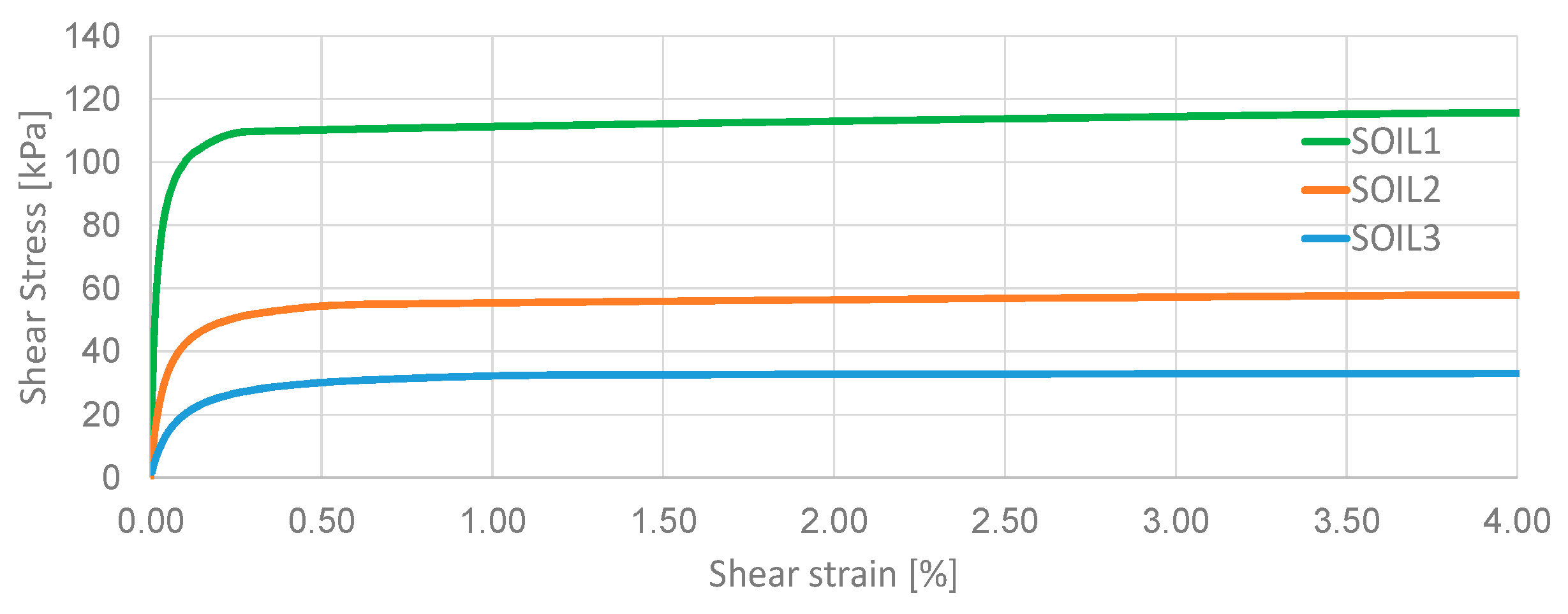
| SOIL1 | SOIL2 | SOIL3 | |
|---|---|---|---|
| Mass density (Mg/m3) | 2.0 | 1.7 | 1.5 |
| Shear Modulus (kPa) | 7.2 × 10⁵ | 1.53 × 10⁵ | 6 × 10⁴ |
| Bulk Modulus (kPa) | 1.56 × 10⁶ | 3.32 × 10⁵ | 3 × 10⁵ |
| Cohesion (kPa) | 100 | 50 | 37 |
| Shear wave velocity (m/s) | 600 | 300 | 200 |
| εSd (mm/mm) | |||||
|---|---|---|---|---|---|
| OD (mm) | t (mm) | fY (MPa) | Low Safety Class | Medium Safety Class | High Safety Class |
| 254 | 12.7 | 448 | 3.0 × 10⁻² | 2.44 × 10⁻² | 1.85 × 10⁻² |
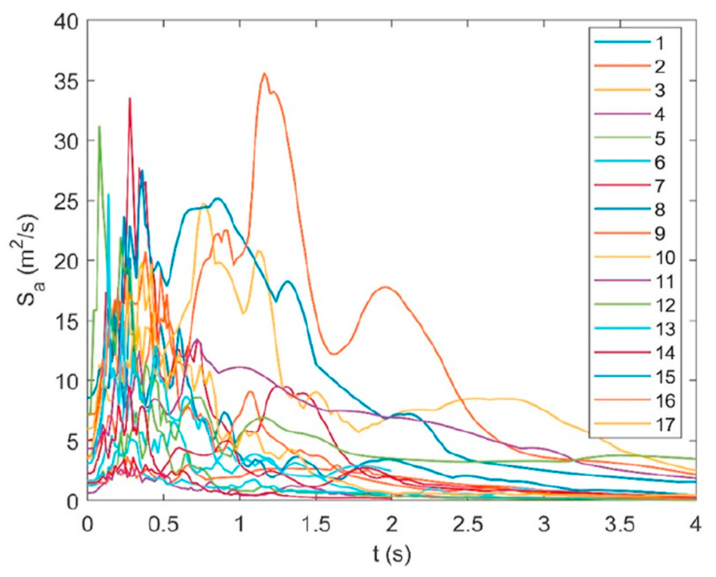
| Input Motion | Station | PGA [g] | Duration [s] |
|---|---|---|---|
| 1 | BORREGO | 1.24 | 40.00 |
| 2 | AZE | 1.66 | 40.00 |
| 3 | CAP | 5.01 | 40.00 |
| 4 | CNP | 3.53 | 25.00 |
| 5 | H-PVB | 3.68 | 40.00 |
| 6 | SCS | 6.00 | 40.00 |
| 7 | BLC | 0.66 | 40.00 |
| 8 | H-COS | 1.44 | 40.00 |
| 9 | H-CAL | 1.26 | 40.00 |
| 10 | A-KOD | 1.51 | 21.00 |
| 11 | Northridge | 8.57 | 15.00 |
| 12 | Takatori | 7.20 | 40.00 |
| 13 | Llolleo | 3.54 | 116.50 |
| 14 | Erzican | 4.33 | 18.00 |
| 15 | Lucerne Valley | 7.12 | 40.00 |
| 16 | Imperial Valley | 3.09 | 22.00 |
| 17 | Trinidad | 2.28 | 21.40 |
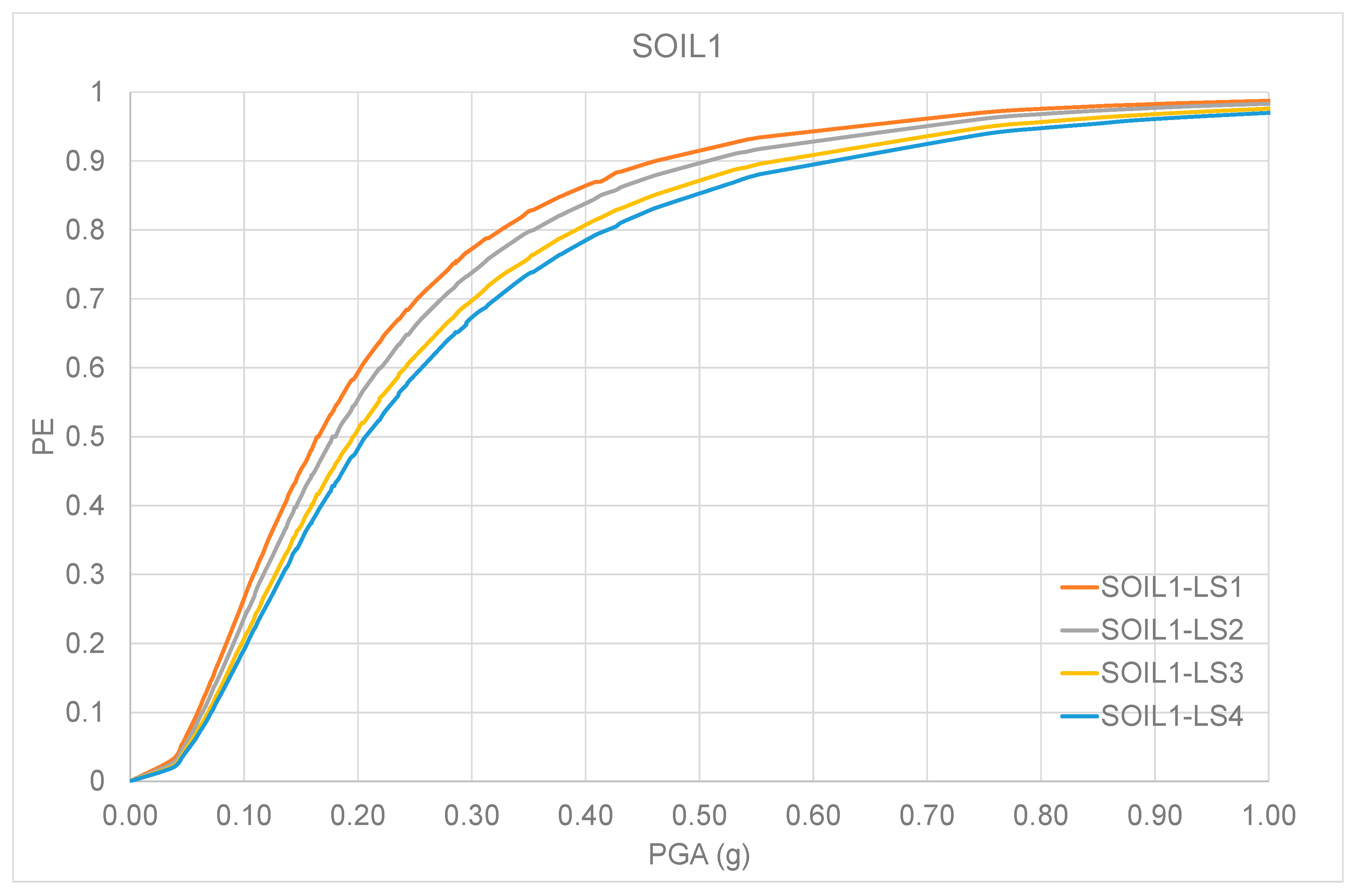
| SOIL1 | LS1 | LS2 | LS3 | LS4 |
|---|---|---|---|---|
| β | 0.793 | 0.809 | 0.821 | 0.833 |
| μ | 0.165 g | 0.176 g | 0.196 g | 0.207 g |
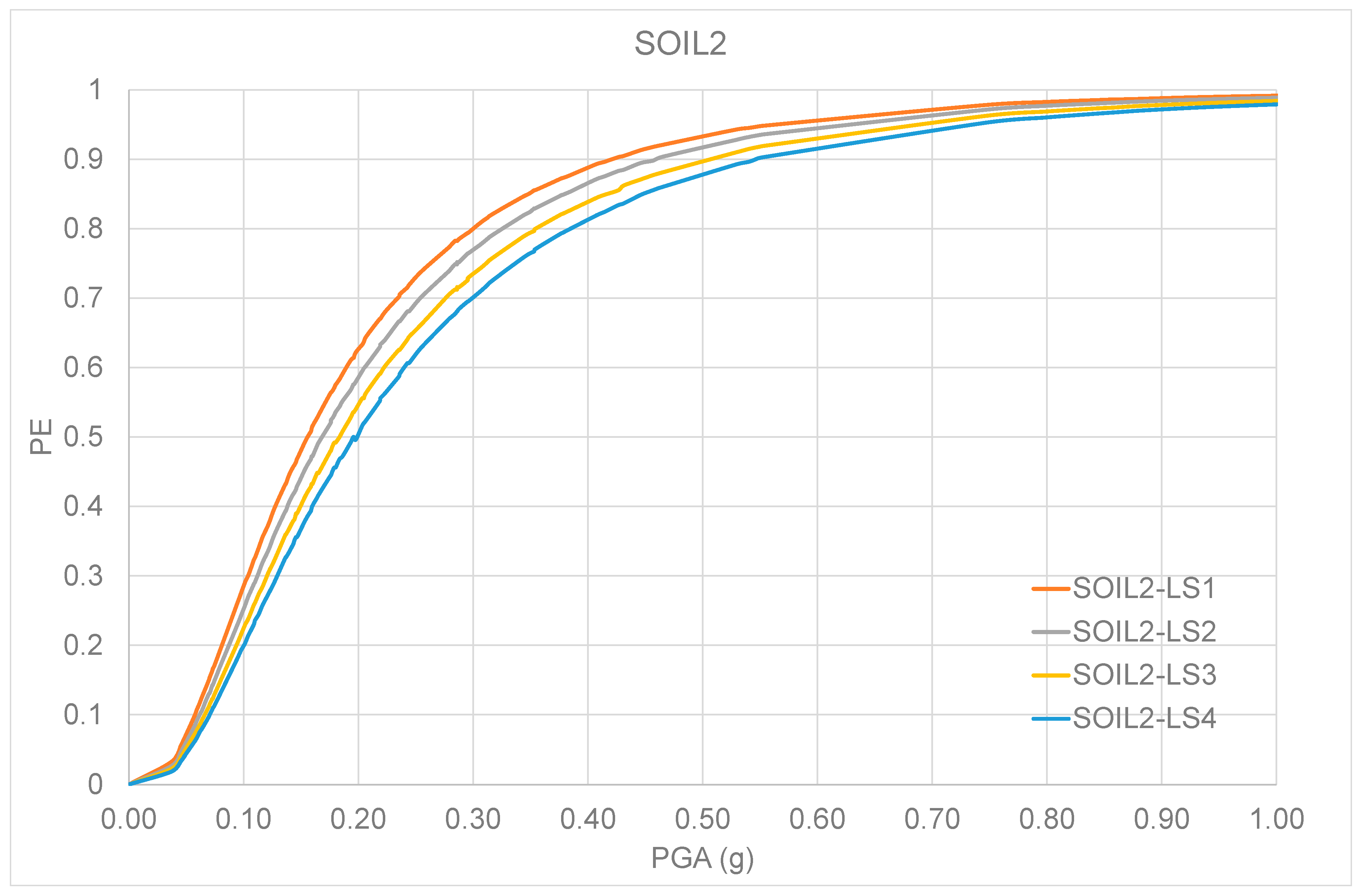
| SOIL2 | LS1 | LS2 | LS3 | LS4 |
|---|---|---|---|---|
| β | 0.776 | 0.781 | 0.791 | 0.799 |
| μ | 0.156 g | 0.169 g | 0.183 g | 0.196 g |
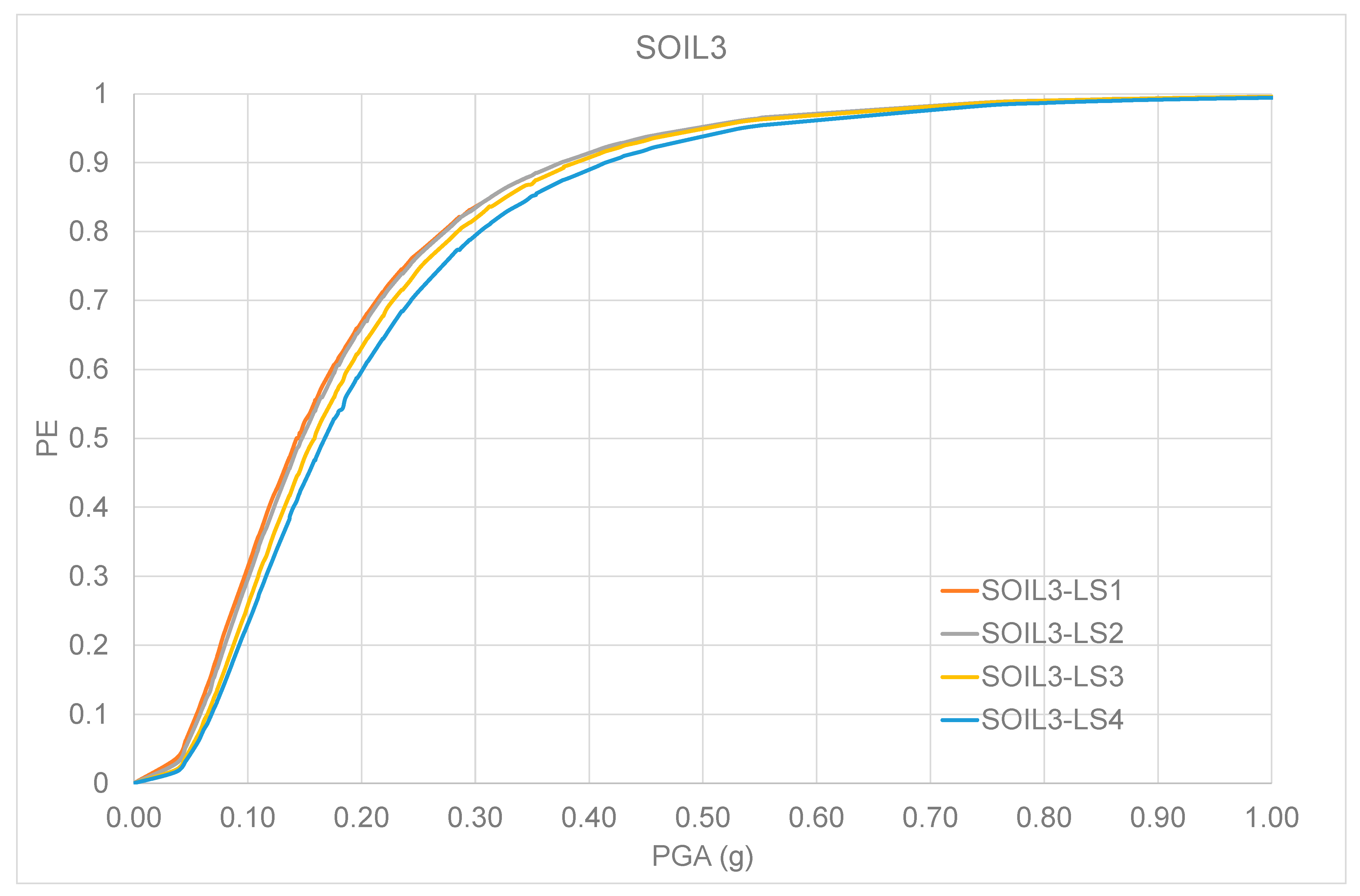
| SOIL3 | LS1 | LS2 | LS3 | LS4 |
|---|---|---|---|---|
| β | 0.749 | 0.728 | 0.670 | 0.705 |
| μ | 0.144 g | 0.149 g | 0.158 g | 0.168 g |
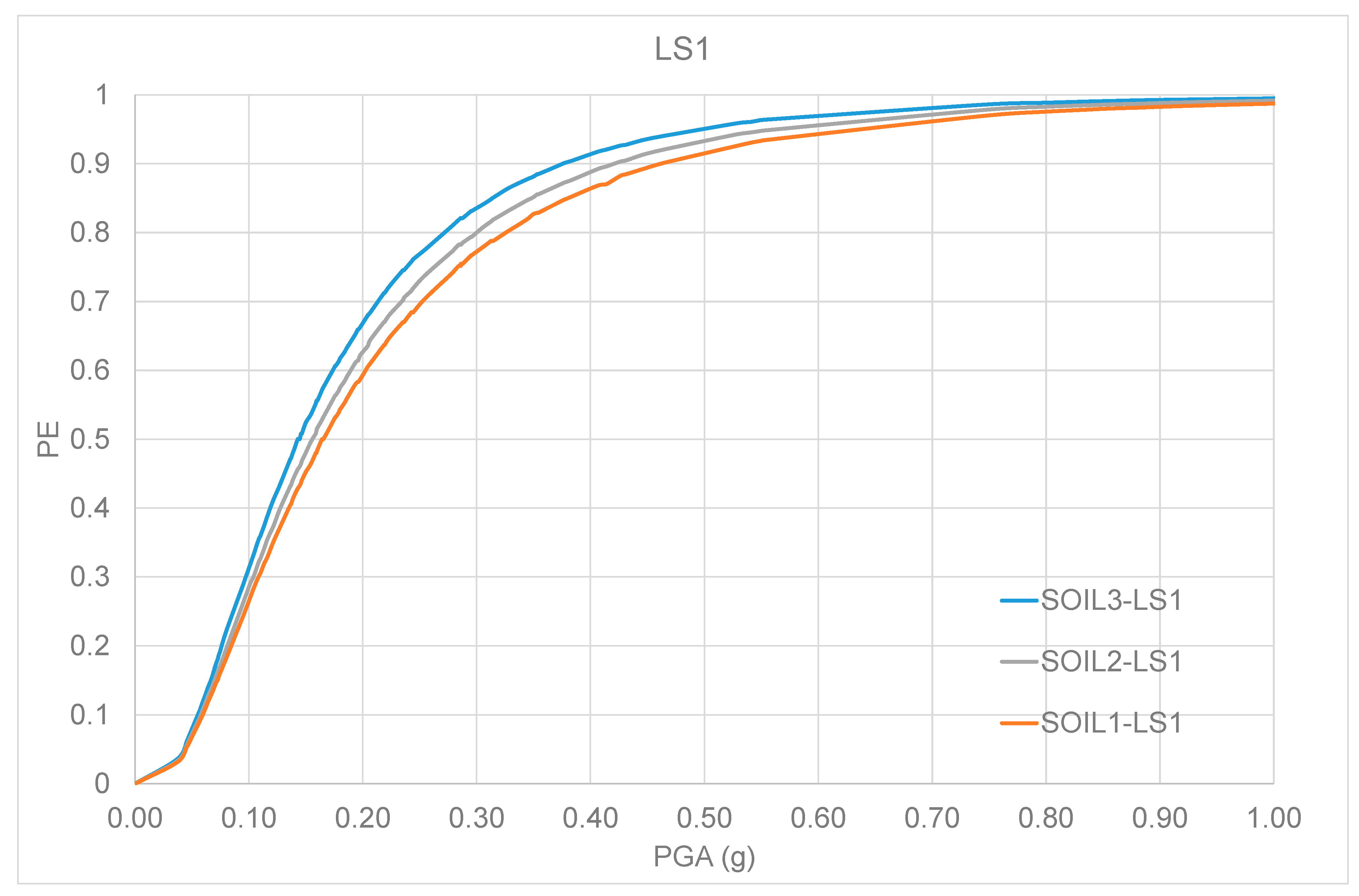
| PGA = 0.30 g | LS1 | LS2 | LS3 | LS4 |
|---|---|---|---|---|
| SOIL1 | 0.77 | 0.73 | 0.70 | 0.68 |
| SOIL2 | 0.80 | 0.78 | 0.72 | 0.70 |
| SOIL3 | 0.84 | 0.83 | 0.81 | 0.79 |
Publisher’s Note: MDPI stays neutral with regard to jurisdictional claims in published maps and institutional affiliations. |
© 2022 by the authors. Licensee MDPI, Basel, Switzerland. This article is an open access article distributed under the terms and conditions of the Creative Commons Attribution (CC BY) license (https://creativecommons.org/licenses/by/4.0/).
Share and Cite
Forcellini, D.; Mina, D.; Karampour, H. The Role of Soil Structure Interaction in the Fragility Assessment of HP/HT Unburied Subsea Pipelines. J. Mar. Sci. Eng. 2022, 10, 110. https://doi.org/10.3390/jmse10010110
Forcellini D, Mina D, Karampour H. The Role of Soil Structure Interaction in the Fragility Assessment of HP/HT Unburied Subsea Pipelines. Journal of Marine Science and Engineering. 2022; 10(1):110. https://doi.org/10.3390/jmse10010110
Chicago/Turabian StyleForcellini, Davide, Daniele Mina, and Hassan Karampour. 2022. "The Role of Soil Structure Interaction in the Fragility Assessment of HP/HT Unburied Subsea Pipelines" Journal of Marine Science and Engineering 10, no. 1: 110. https://doi.org/10.3390/jmse10010110