Abstract
Considering the nature of marine accidents, even a single accident can result in significant damage to the environment and property, as well as loss of life. Therefore, the initial response should be rapid and accurate, and various decision support systems have been developed to achieve this. Research on simulating progressive flooding on board immediately after an accident is being actively conducted, but this requires high levels of computing power. In this study, a methodology for converting simulated ship motion data into a ship motion database is presented. The model of a training ship from the Korea Institute of Maritime and Fisheries Technology and KRISO in-house code SMTP was used for ship motion computations. The short-time Fourier transform was used to convert time-series motion data into a spectrogram motion database. A methodology for deriving a predicted location of the damage center is presented. The candidate locations of the damage centers were obtained by comparing the root mean square error values of the ship motion database from the simulation and real-time ship motion data. Finally, a probability function was suggested to confirm the predicted location of the damage center. Using 100 randomly selected test cases, our method showed 95% accuracy.
1. Introduction
Considering the nature of marine accidents, even a single accident can result in significant damage to the environment and property, and, most importantly, loss of life. Table 1 shows the number of marine accidents that occurred in Korea between 2016 and 2020, categorized by accident type. Human errors accounted for 77.5% of the causes [1]. Hence, the development of appropriate decision support systems and accident response systems for decision makers is crucial [2].

Table 1.
Summary of marine accidents in Korea between 2016 and 2020.
During maritime accidents, the initial response plays a significant role in minimizing damage. When the initial response fails, the amount of damage and casualties increase rapidly. Therefore, the safety of the crew should be maintained through an efficient response in the early stages of an accident. Rapid accident detection is necessary to respond quickly. Next, the scale of accidents over time should be provided to decision makers by predicting the progressive extent of the flooding area. Subsequently, an appropriate response procedure should be developed based on the current status and prediction results [3].
Using flooding sensors is the fastest and easiest way to detect the flooding location. Research on the detection of flooding casualties using various sensors, including flooding sensors, was conducted [4,5]. To appropriately use a flooding-sensor-based system, it is necessary to install sufficient flood sensors onboard and monitor and control the operation of the sensors. However, it is practically difficult to install a sufficient number of flooding sensors to guarantee safety, and it is more difficult to apply them to existing ships that have no flooding sensors. Additionally, it is even more difficult to guarantee the normal operation of the sensors during accidents.
The development of time-domain progressive flooding simulation tools is underway, which is operated on board as a way to help decision makers make decisions after detecting flooding locations [6,7,8,9,10,11,12,13]. These simulation tools implement virtually progressive flooding scenarios in a complex onboard structure. Through the identified current situation and the simulation results of progressive flooding, the decision maker appropriately responds to an accident. However, this method requires high computing power because a large number of calculations must be performed quickly for the simulation.
Therefore, a finite number of damage cases within the probable range among the operating conditions was defined and simulated [14]. Through the simulation, time-series data for each case were obtained and converted into a ship motion database. When an accident occurs, the most similar case can be searched in the database and referred to for decision making. In this study, a methodology for converting simulated ship motion data into a ship motion database was proposed, along with a methodology for predicting the location of the damage center through a comparison between a ship motion database from the simulation and real-time ship motion data.
2. Materials and Methods
Herein, we suggest a method that predicts the location of the damage center through spectral analysis of the damaged ship’s motion. The method is divided into the construction of the ship motion database and the probabilistic prediction of the damage location.
The ship motion database is based on the damaged ship’s motion time-series data simulated under several conditions. To convert time-series data into a database, the short-time Fourier transform (STFT) was applied to the time-series data, and the spectrogram matrices, i.e., the output of the STFT, were stored as a ship motion database.
Then, the location of the damage center was predicted by comparing the ship motion database and the real-time motion data. Among the several predicted damage centers obtained from each heave, roll, and pitch motion database, the location of the damage center with the highest probability was predicted, and for that, a probability function was suggested. This section describes the methodology used in the study.
2.1. Short-Time Fourier Transform and Spectrogram
Most sounds and vibrations are complex waves that combine two or more waveforms. The components that form such waves can be classified as periodic waves using a Fourier transform. The Fourier transform and its inverse are used to map any function in the interval −∞ to +∞ in either the time or frequency domain into a continuous function in the inverse domain. In practice, data are always available in the form of a sampled time function, represented by a time series of amplitudes separated by fixed time intervals of limited duration. When dealing with such data, a modification of the Fourier transform, i.e., the discrete Fourier transform (DFT), is used. The fast Fourier transform (FFT) is the efficient computation of the DFT implementation, where its fast computation is considered an advantage. FFT performs well for the estimation of periodic signals in the stationary state; however, it does not perform well for the detection of sudden or fast changes in the waveform [15].
The STFT allows us to perform time-frequency analyses. It is used to generate representations that capture both the local time and the frequency content in the signal. Similar to the Fourier transform, the STFT relies on fixed basis functions; however, it uses fixed-size time-shifted window functions to transform the signal and can be expressed as
where is the amount of shift and is the number of samples [16].
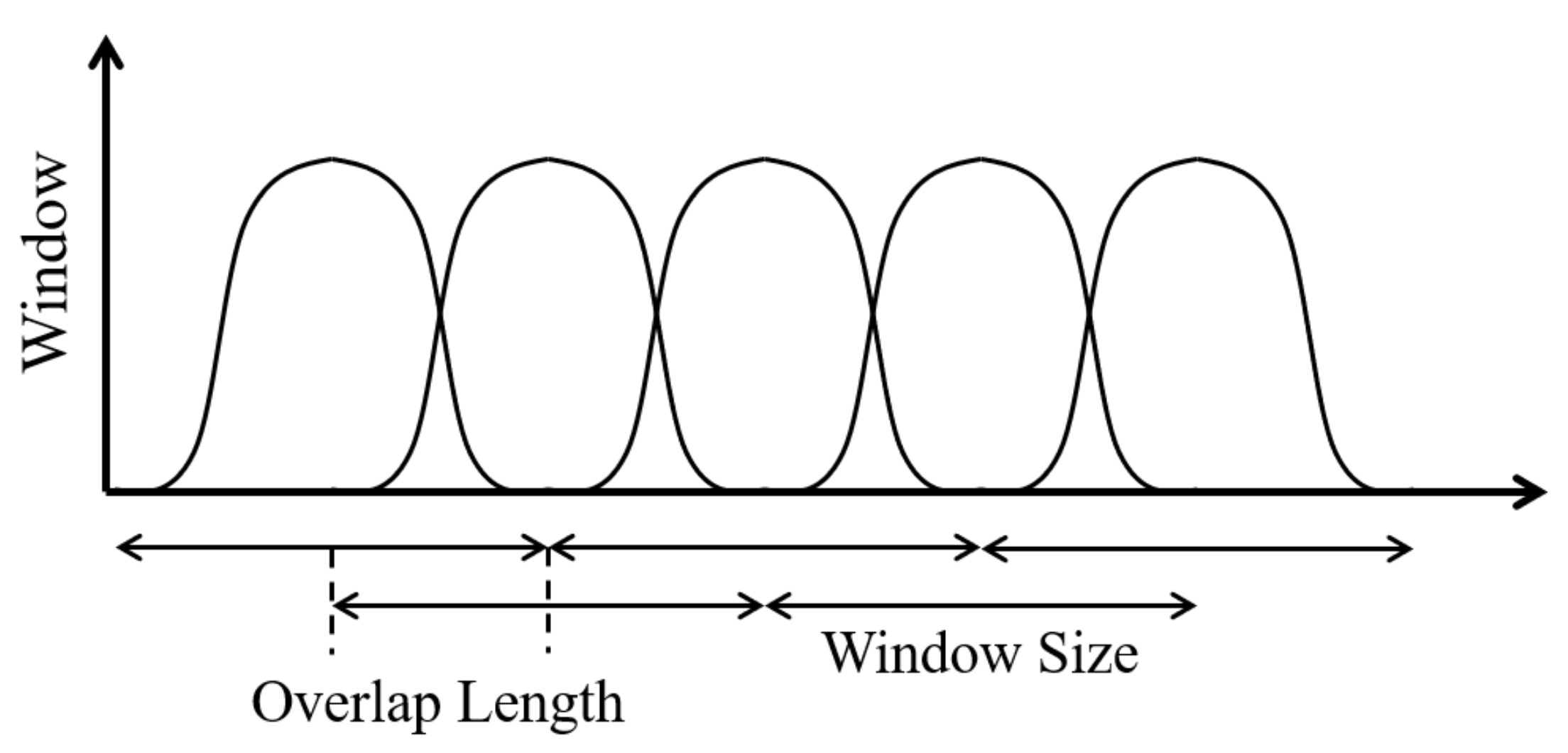
A spectrogram of STFT represents the normalized squared magnitude of the STFT coefficients [17]. Hence, the energy in the time-frequency signal is equal to the energy in the spectrogram of the STFT. In STFT, the time-domain signals are divided into smaller parts (windows), and the Fourier transform is computed for each windowed section to obtain the frequencies. Some segments can overlap with each other to produce smooth and comprehensive output data [18]. Overlapping, as shown in Figure 1, indicates that consecutive windows overlap when obtaining data corresponding to a specific window size ().
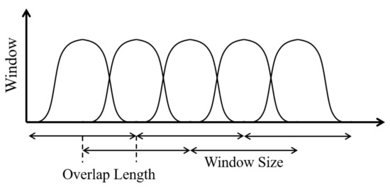
Figure 1.
Window size and overlap length of the window function for STFT.
2.2. Probability Density Function of the Normal Distribution
The normal distribution, also referred to as the Gaussian distribution, is the most important continuous distribution. For −∞ < < +∞ and > 0, when is the mean and is the standard deviation, the normal distribution is denoted by , and its probability density in the domain is given by
The maximum probability value is located on the mean, and the value is a function of the standard deviation, as shown in Equation (3):
The fact that Equation (2) is integrated to give an area of 1 can be proven using the Gaussian integral as
Here, the variables of integration are changed from to (i.e., ).
The constants and included in the normal distribution correspond to the expectation and standard deviation :
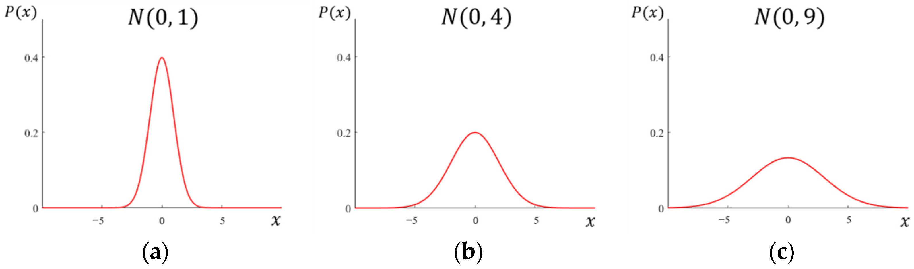
The probability density functions of for , illustrated in Figure 2, show that the normal density is symmetric and bell-shaped. Furthermore, as shown in Figure 2, a low standard deviation indicates that the data tend to be adjacent to the mean, whereas a high standard deviation indicates that the data are widely distributed [19].
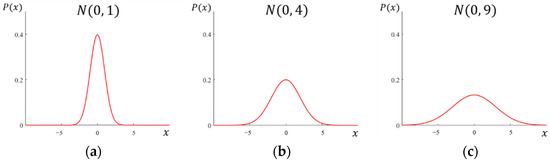
Figure 2.
Probability density functions of normal density : (a) , (b) , and (c) .
Using the characteristics of the probability density function of a normal distribution, in this study, the location of the damage center in two-dimensional coordinates, namely, the vertical and longitudinal positions of the ship’s compartments, was predicted. The probability function is shown in Equation (7), and its plot is shown in Figure 3. The probability function is a three-dimensional function obtained by rotating a two-dimensional probability density function of normal distribution by 180° at a line that passes through a point at (x = a, z = b) and is perpendicular to the x–z plane.
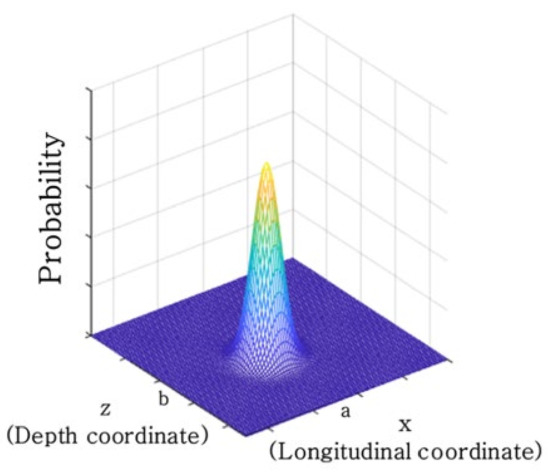
Figure 3.
Probability function applied to predict the location of the damage center.
Here, the function indicates the probability of damage at the (x, z)-coordinates when the predicted damage center is (a, b) and is the standard deviation.
When predicting the damage location through this method, several predicted damage locations are obtained through comparison with the heave, roll, and pitch motion databases. The probability function is used instead of simply using a majority when determining the final predicted damage location. The advantage of using the probability function is that (1) it can consider the possibility of damage to the predicted location’s surroundings, not just at the location; (2) better results can be obtained than a simple majority; and (3) the probability function values generated for each iteration can be stored and delivered for reference to the next prediction iteration.
3. Case Study
3.1. Ship Motion Data
3.1.1. Ship Specifications
The ship used in this study is a training ship from the Korea Institute of Maritime and Fisheries Technology, and its structure is shown in Figure 4. It is a 5200-ton ship with dimensions of 145 m length overall (LOA), 18 m breadth, and 7.5 m depth, and the simulation was performed using this ship [14].
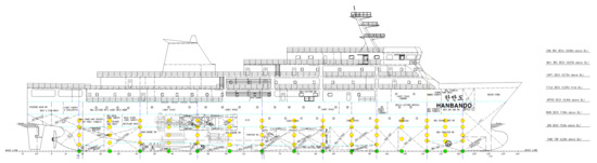
Figure 4.
Simulated ship model profile and the locations of damage centers.
3.1.2. Construction of Ship Motion Data
In this study, we simulated the ship motion under various combinations of conditions. The conditions included the locations of the damage centers, sizes of the damaged area, sea states, and angles of regular incident waves. In order to compute damaged ship motion, SMTP code was used. SMTP is an in-house code of KRISO and was used with flooding rates found using the Bernoulli equation and empirical discharge coefficients. The floodwater in compartments can be modeled either with a horizontal free surface or with a dynamic model in which the pendulum model is used for the center of gravity and resulting inclined free surface. The compartments are treated independently; therefore, the model can be selected appropriately to represent the property of each compartment. Ship motions are calculated using 6DOF non-linear equations in the time domain in which the Froude–Krylov and restoring forces are calculated for an instantaneous wetted surface, and the hydrodynamic forces are calculated by the traditional strip method. The floodwater affects the ship’s motion as internal forces, not the external forces; in other words, it changes the mass and its center of gravity, resulting in changes of the inertial and gravity forces. Details are presented in [20]. It was a simulation without thrust by the propeller; therefore, the initial velocity of the ship was zero.
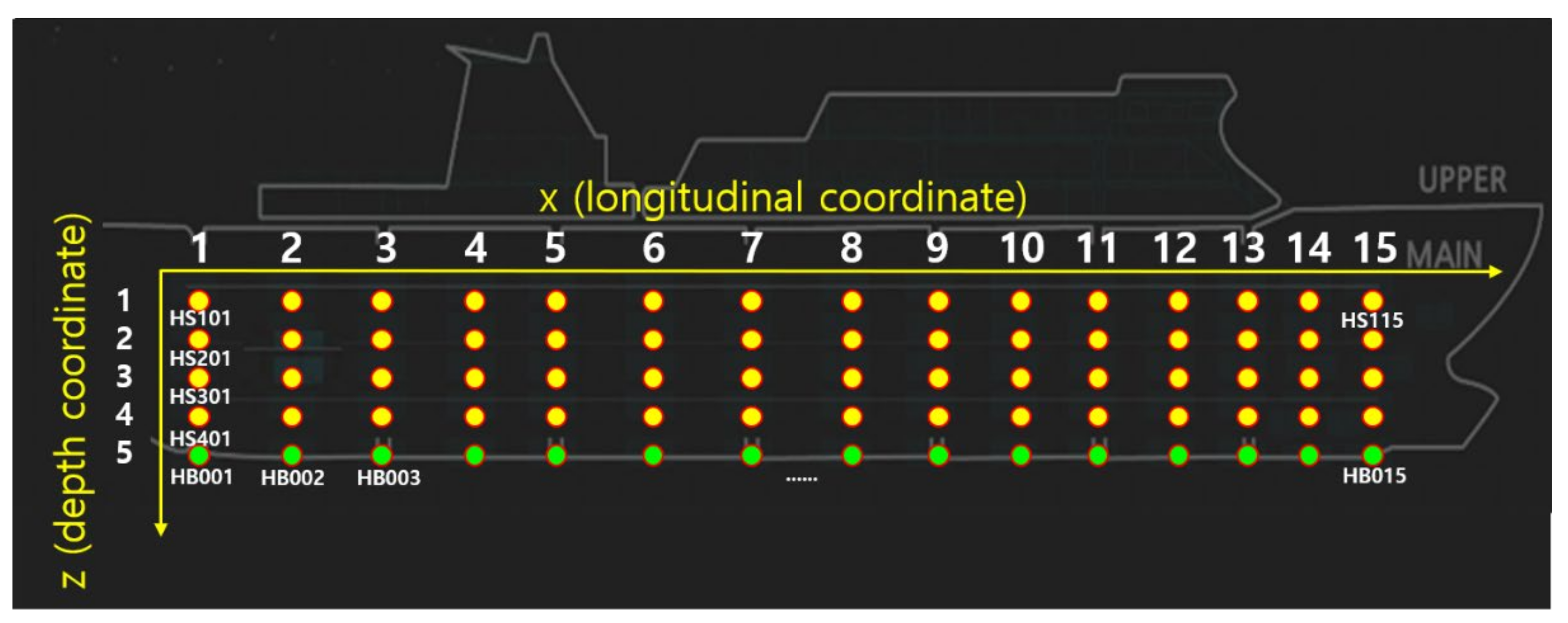
As shown in Figure 5, there were 15 locations in the longitudinal direction and five locations in the depth direction of the ship profile, giving a total of 75 damage locations. This damage location is indicated by a three-digit number in Figure 5. Yellow circles indicate locations of damage centers on the hull side, and green circles indicate the locations of damage centers at the hull bottom. At each depth level, starting with the stern, the three-digit numbers for the damaged locations increase by one when moving toward the stem. The uppermost points were considered to be from locations 101 to 115, and this became 201, 301, and 401 when moving toward the bottom of the ship. Damage to the hull bottom of the ship was identified by locations from 001 to 015.
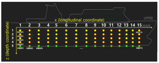
Figure 5.
Identification of locations of damage centers using 3-digit codes and a coordinate system.
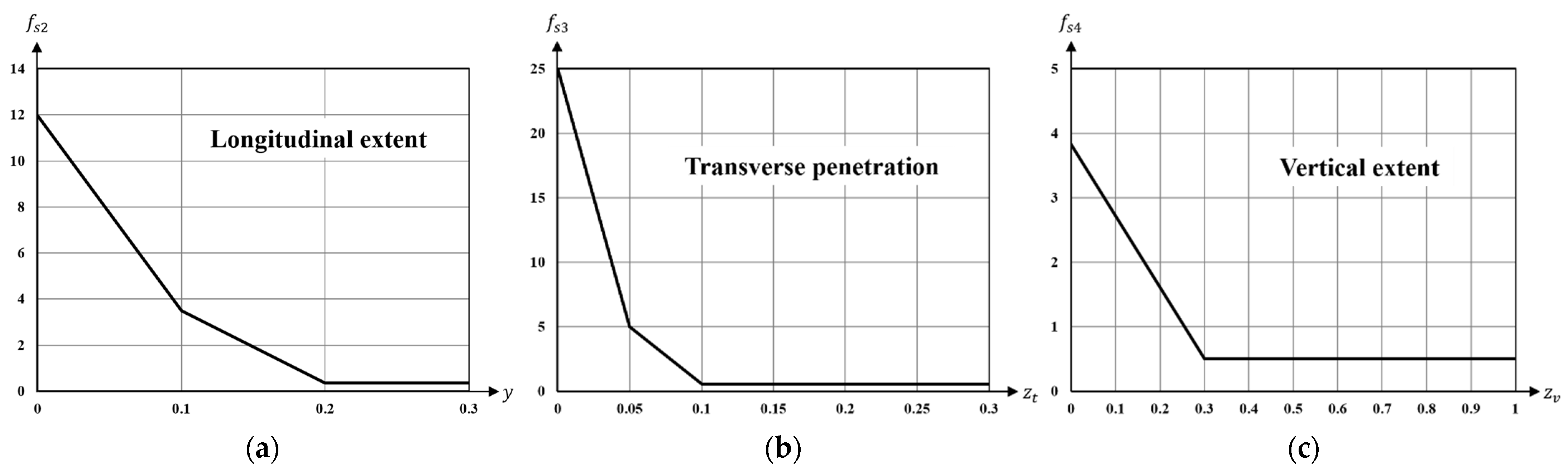
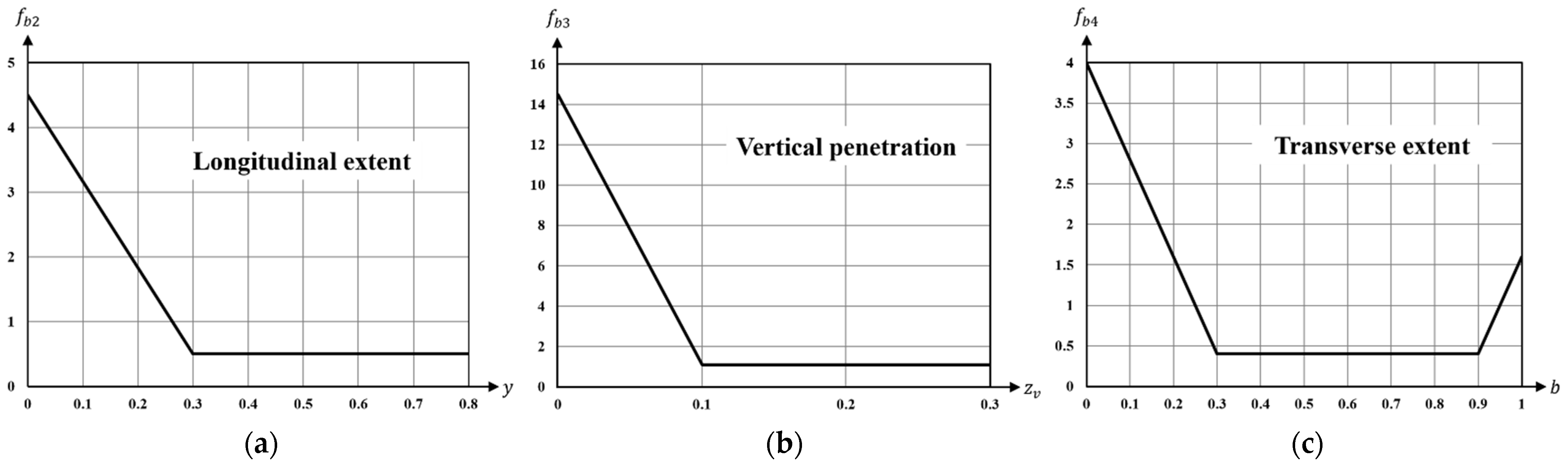
The size of the damaged area was classified as 30%, 70%, and 100% of the maximum hole size. The maximum hole size of the side damage is defined by statistical data as the dimensionless ratio of longitudinal extent, transverse penetration, and vertical extent to the hull specification, as shown in Figure 6. The maximum hole size of the bottom damage is defined by statistical data as the dimensionless ratio of the longitudinal extent, vertical penetration, and transverse extent to the hull specification, as shown in Figure 7 [21].

Figure 6.
Side damage due to collision: (a) density distribution functions of longitudinal extent, (b) density distribution functions of transverse penetration, and (c) density distribution functions of vertical extent.

Figure 7.
Bottom damage due to stranding: (a) density distribution functions of longitudinal extent, (b) density distribution functions of vertical penetration, and (c) density distribution functions of transverse extent.
Therefore, the maximum hole size at the side of the ship after a collision is defined in this study using Equation (8), and the maximum hole size at the bottom of the ship after ship grounding is defined using Equation (9):
Here, L is the LOA, D is the depth, and B is the breadth.
The sea states were specified by the average wave height and average wave period corresponding to sea states 4, 5, and 6 from Table 2. Finally, the incident angles of the regular wave used for the simulation were divided into eight directions from 0° to 315° at 45° intervals. Combining the above conditions, a total of 5400 datasets were created. Each dataset contained six degrees of freedom (6DOF) for the ship motion (surge, sway, heave, roll, pitch, and yaw) for 1 h at intervals of 0.5 s.
Table 2.
Significant wave height and spectral peak period applied to the simulation.
By combining these conditions, each time-series data file name followed the following rule:
Here, indicates the hull side damage, and indicates the hull bottom damage. numbers signify the three-digit numbers for the damaged locations. indicates the hole area and the numbers signify the three-digit number of percentages of the damaged hole area per statistical maximum hole size. indicates the sea state and the numbers are 04, 05, or 06. indicates the incident regular wave angle and the numbers signify the three-digit number from 000 to 315 at 45 intervals.
For the rolling angle above the downflooding angle, flooding occurs in non-watertight and other openings, allowing the ship to capsize and sink with the loss of additional dynamic stability. The downflooding angle refers to the static angle from the intersection of the vessel’s centerline and the waterline in calm water to the first opening that cannot be closed and, through which, downflooding can occur [22]. Therefore, a roll motion of 45°, which is the downflooding angle of the model for this study, was defined as the standard for capsizing and sinking. A total of 2181 cases among the 5400 cases were capsized in a 1 h simulation. Furthermore, the maximum peak-to-peak heave amplitude was 25.1 m in the case of HS203HA100_SS06WA180 and the maximum peak-to-peak pitch amplitude was 77.8° in the case of HS402HA070_SS06WA135 among all cases.
3.2. Construction of Spectrogram Database
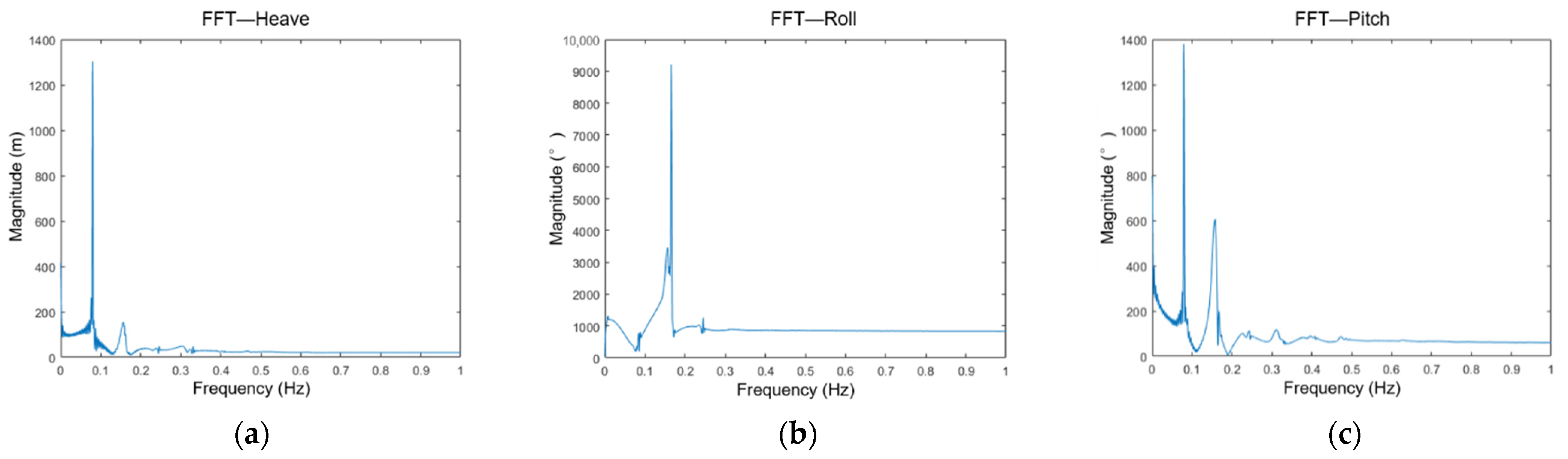
The heave, roll, and pitch, which can be characterized by the periodic motion among the other 6DOF hull motion data, can be considered complex waves, which are combinations of two or more waves. These complex waves can be classified as periodic or non-periodic waves. The components of these complex waves can be observed in the spectrum. If the time-series data with the x-axis set to time and the y-axis set to the amplitude are converted into a spectrum, then a spectrum with frequency on the x-axis and amplitude on the y-axis can be obtained. The FFT is widely used in spectrum analysis for time-series data, and from this, the type and number of simple waves that form the whole complex waves can be determined [23].
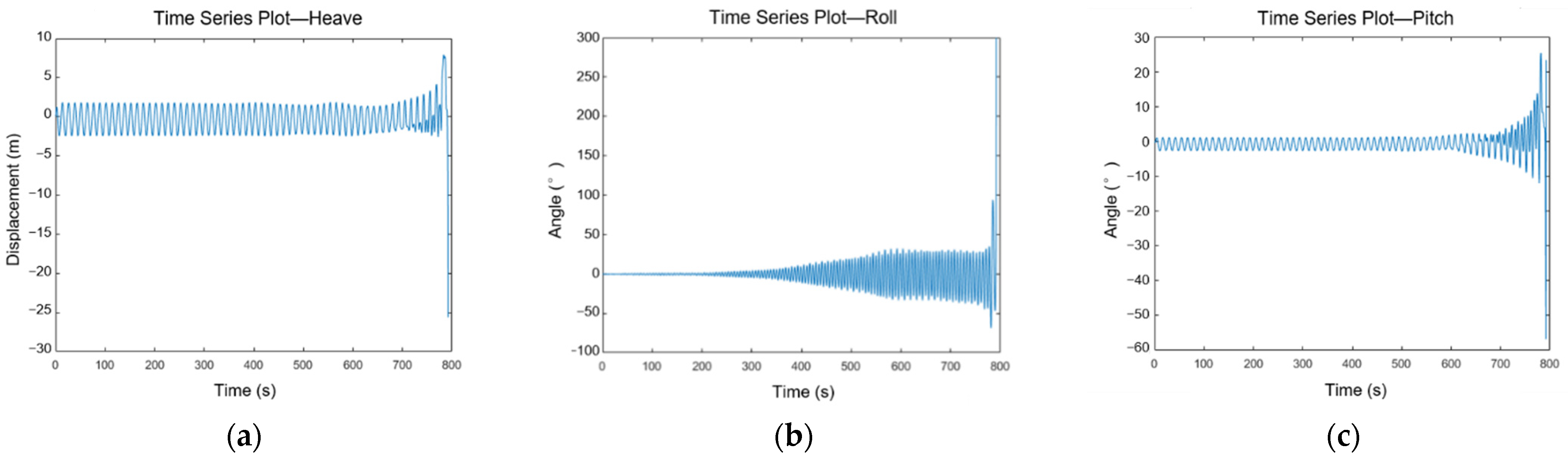
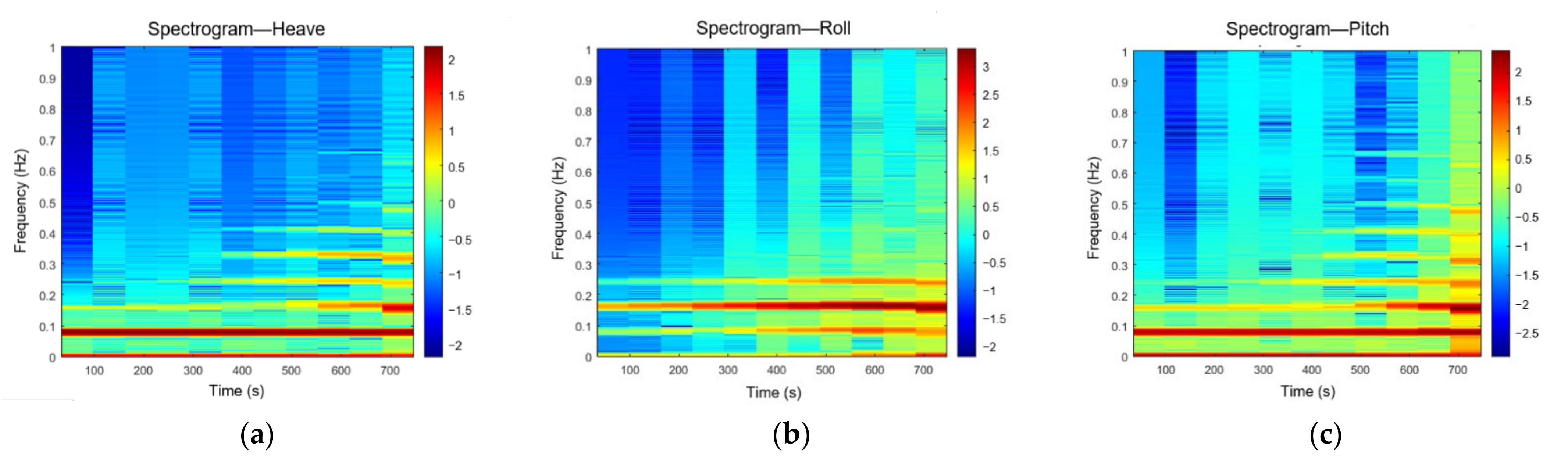
However, simple spectra could not be used in this study because the ship motion data components varied with time. Thus, the ship motion database was constructed using STFT and spectrograms that showed the changes in frequency over time. Figure 8 shows the simulated heave, roll, and pitch motion data file HB001HA100_SS06WA135, which represented the simulation for a ship with damage corresponding to 100% of the maximum hole size at location 001 at the hull bottom in sea state 6 and a regular incident wave angle of 135°. Under these conditions, the simulated ship sunk within approximately 15 min. The plots for the FFT and STFT results of the HB001HA100_SS06WA135 time-series data are shown in Figure 9 and Figure 10, respectively.
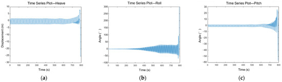
Figure 8.
Simulated time-series motion plots of the case HB001HA100_SS06WA135: (a) heave time-series plot, (b) roll time-series plot, and (c) pitch time-series plot.
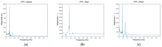
Figure 9.
FFT plots of the case HB001HA100_SS06WA135: (a) FFT plot for heave, (b) FFT plot for roll, and (c) FFT plot for pitch.
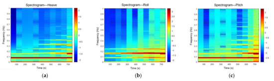
Figure 10.
Spectrogram of the case HB001HA100_SS06WA135: (a) spectrogram for heave, (b) spectrogram for roll, and (c) spectrogram for pitch.
3.2.1. STFT Specifications
The STFT was performed with the following specifications: as the time-series data were recorded with a 0.5 s interval, the sampling frequency, which indicates how much discrete data exist in one second, was set to 2. The window size was specified as 260 samples (i.e., data obtained for 130 s in one window), and the frequency resolution was set to two to the power of 10 (210) using empirical methods. The Hamming window formula, which is shown in Equation (11), was used for the sliding window:
Here, n is the number of windows and is the length of the window function [24].
In addition, the time resolution was improved by applying a 50% overlap to the windows.
3.2.2. Method for Database Construction
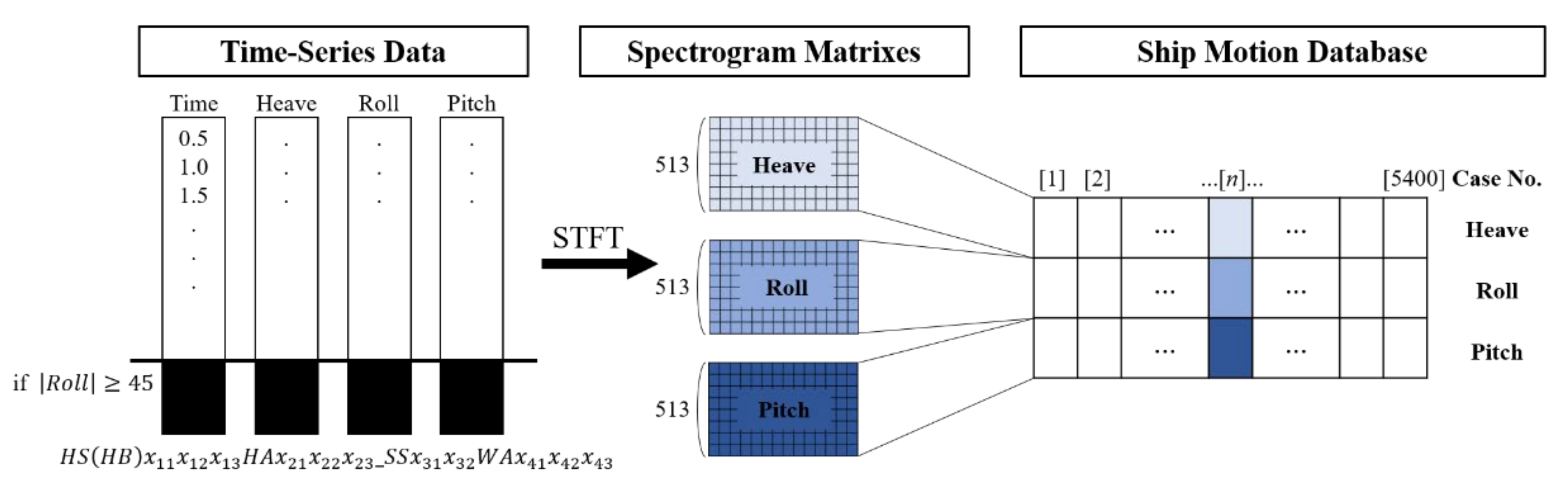
As shown in Figure 11, the ship motion database was constructed by converting time-series motion data into a spectrogram. First, it was assumed that the ship sank after the roll angle exceeded the downflooding angle (45° as defined above); therefore, the data after the first appearance of the 45° roll angle were removed. Next, using the STFT specification defined above, the spectrogram matrix was obtained by performing an STFT on the heave, roll, and pitch time-series data. To perform an STFT, a function called “spectrogram” in MATLAB (v.R2021a, Natick, MA, USA) was used. The number of rows of the matrix was , which made it a matrix with 513 rows in this study. The matrices for 5400 cases were stored in each array of the heave, roll, and pitch motion databases.

Figure 11.
Procedure for ship motion database construction.
3.3. Prediction of Damage Center
3.3.1. Test Data Production
The test datasets were produced assuming the following scenario: shortly after the ship at sea recognized that an accident had occurred, the location of the damage center was predicted by comparing the real-time motion data with the motion database.
For N randomly selected cases from 5400 damage cases, the test datasets were produced after deleting some of the initial parts and then performing the STFT. Some of the initial data were deleted to ensure that the data in the database and the data to be used for testing were different. Considering a 50% overlap, the initial deleted data should be less than 130 samples and, simultaneously, not too much data should be deleted to prevent a lack of data for prediction. Thus, the initial 17 samples, which were co-prime integers with 130, were deleted before the STFT. The number 17 was decided empirically to generate the test datasets that were as different as possible from the database. In other words, the data obtained in real time at sea could not be the same as the databases; therefore, some of the initial data were deleted, and the test data, which were different from the database, were produced.
The window size was 260 samples and was processed using 130 overlapping samples. An STFT was performed on every sequential 260 samples of each heave, roll, and pitch time-series data collected for 130 s, as the motion data were collected every 0.5 s. As a result, a spectrogram matrix was obtained, which is an array of column vectors. Each column vector is called a “p-vector.” The number of rows of the spectrogram matrix was . In this study, since the frequency resolution was set to , the p-vector was a column vector with 513 rows. A p-vector contained information on the frequency components of the finite complex wave for a number of samples that is the same as the window size. The procedure for the test dataset production is illustrated in Figure 12.
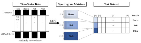
Figure 12.
Procedure for test dataset production.
3.3.2. RMSE to Predict Damage Center
In this study, the RMSE was used to compare the motion database and real-time data. Figure 13 shows the procedure for calculating the RMSE between the motion database and the test dataset. It was assumed that the real-time motion data were input by sequentially bringing p-vectors from the first to -th columns of the k-th test dataset among the total N test datasets. is the number of columns in the spectrogram matrix of the k-th test dataset. Since 40.3% of the 5400 cases sunk within 1 h according to the simulations, the number of column vectors was different for each case. Here, D is H when heave was considered, R when roll was considered, and P when pitch was considered.
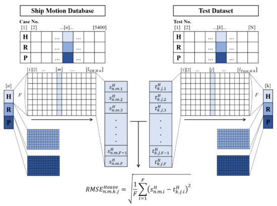
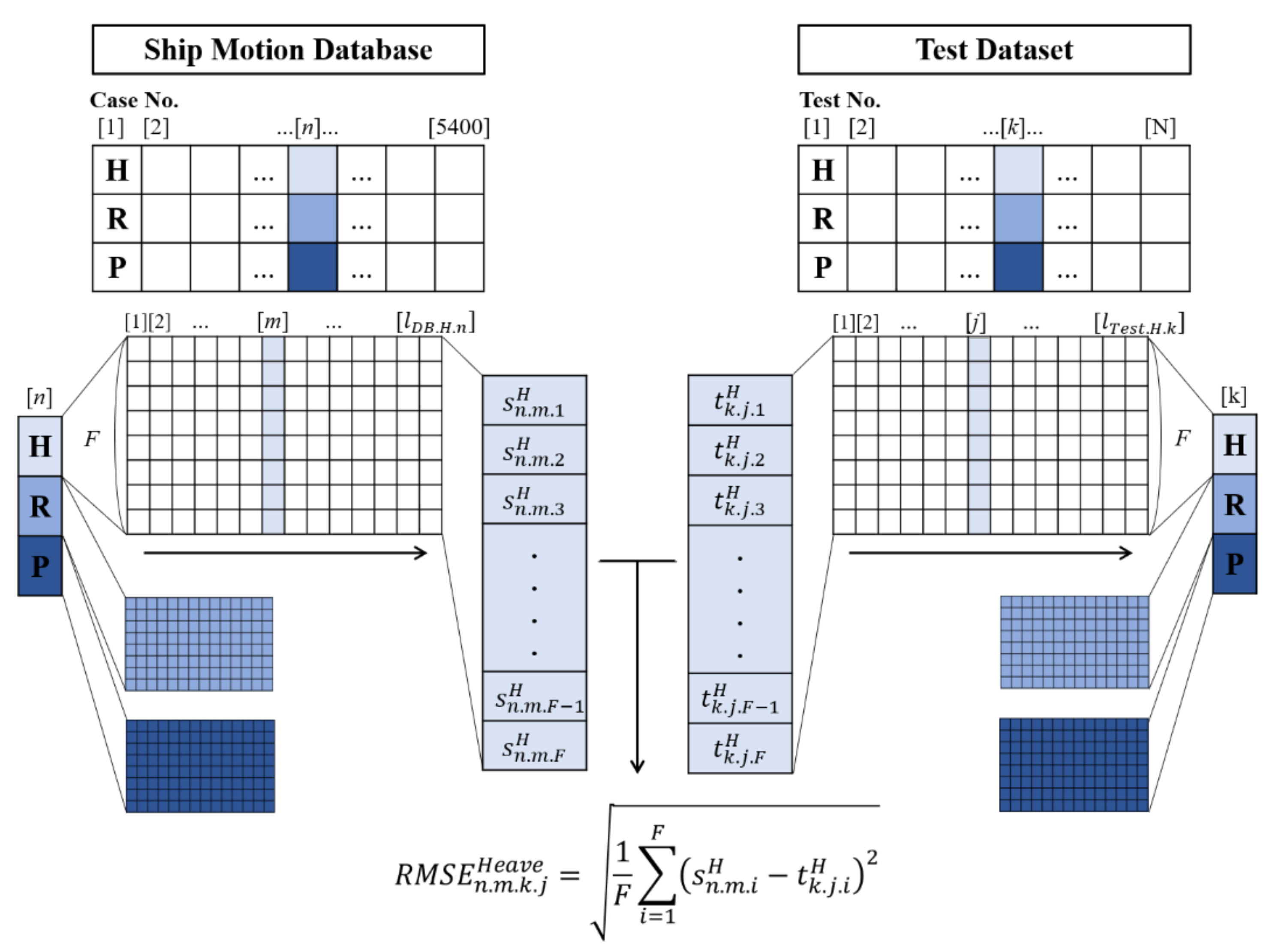
Figure 13.
Procedure of the RMSE calculation between the motion database and the test datasets.
In the first iteration of the k-th test dataset, we first calculated the RMSE between the first p-vectors of the heave, roll, and pitch spectrogram matrices of the k-th test dataset and ship motion database. As shown in Figure 13, the RMSE is calculated one-to-one with all p-vectors of the spectrogram matrix in all cases of the ship motion databases and the p-vectors of the test dataset. The spectrogram matrix of the n-th case contains columns.
For example, , which was the RMSE for the m-th p-vector in the n-th case of the ship motion database in the j-th iteration of the k-th test dataset, could be calculated using Equation (12):
Here, F is the number of columns of the spectrum matrix, which can be calculated using Equation (13).
refers to the entry of the i-th row in the m-th p-vector among the spectrum matrix of the n-th case of heave motion in the ship motion database. refers to the entry of the i-th row in the j-th p-vector of the heave spectrum matrix of the k-th test dataset of the total test datasets.
In one iteration, a number of RMSEs equal to the number of all column vectors in the ship motion database for each heave, roll, and pitch motion, respectively, were calculated; in this study, the total number of column vectors for each motion data was 160,565. For every iteration, the location of the damage center at the minimum RMSE value was selected for heave, roll, and pitch, and a total of three locations of damage centers were obtained. was used as another criterion, which meant the sum of the RMSE of heave, roll, and pitch under the same conditions and could be calculated using Equation (14). After the same method, the location of the damage center, where the was minimized, was obtained. Finally, the four locations of the damage centers were obtained using the heave, roll, pitch, and total:
The RMSE is commonly used when dealing with the differences between the estimated or model-predicted values and the actual values. The validity of using RMSE for the study can be represented by statistical data of the distribution of RMSE values, which have large standard deviations, indicating that the entire RMSE values are widely distributed. In other words, the motions between the damaged cases are distinguishable when converted to a spectrogram so that reasonable results can be obtained when compared with the RMSE.
For example, statistical data indicating the distribution of all RMSE values in the test dataset for HS405HA070_SS05WA270 are shown in Table 3. The table shows the average, standard deviation, minimum and maximum values, and the top 1%, 10%, 25%, and 50% of each RMSE value. According to Table 3, the standard deviation corresponding to the heave and total was large, and the minimum value was sufficiently smaller compared to the top 1%. The standard deviation corresponding to the roll and pitch was relatively small, but the minimum value was sufficiently smaller compared to the average and top 1%. In conclusion, since the RMSE values of heave, roll, pitch, and total were all spread widely, it would be reasonable to predict the location of the damage center by the minimum value of the RMSE values.
Table 3.
Statistics on the distribution of RMSE values of case HS405HA070_SS05WA270.
3.3.3. Probability Function for Prediction of Damage Center
The four locations obtained from the RMSE were within 60 points, from 101 to 415, on the hull side and within 15 points, from 001 to 015, at the hull bottom, as shown in Figure 5. These points are represented as coordinates, as shown in Figure 5. Of the three-digit numbers representing each point, the first digit was set as the z-coordinate, followed by two digits as x-coordinates. With this logic, the points on the hull bottom should have zero as their z-coordinates; however, as their locations are close to the points in the 400s, the z-coordinates were set to five in the coordinate system.
Here, for every location of the damage center predicted by calculating the RMSE with the ship motion database in the same iteration, every criterion, which could be heave, roll, pitch, and total, had the same possibility of becoming a correct prediction and could not guarantee a correct prediction in a majority of cases between four criteria. Therefore, we introduced a probability function. As described in Section 2.2, the probability function was defined in Equation (7).
In one iteration, four predicted locations of the damage centers from each motion database were obtained. At the predicted damage center, the possibility of damage was the highest, but this did not mean that only that point can be damaged. If more than two locations of the four predicted locations were repeated, the possibility of damage at that point would be higher. Therefore, we classified the cases of location repetition in the four predicted locations of damage centers.
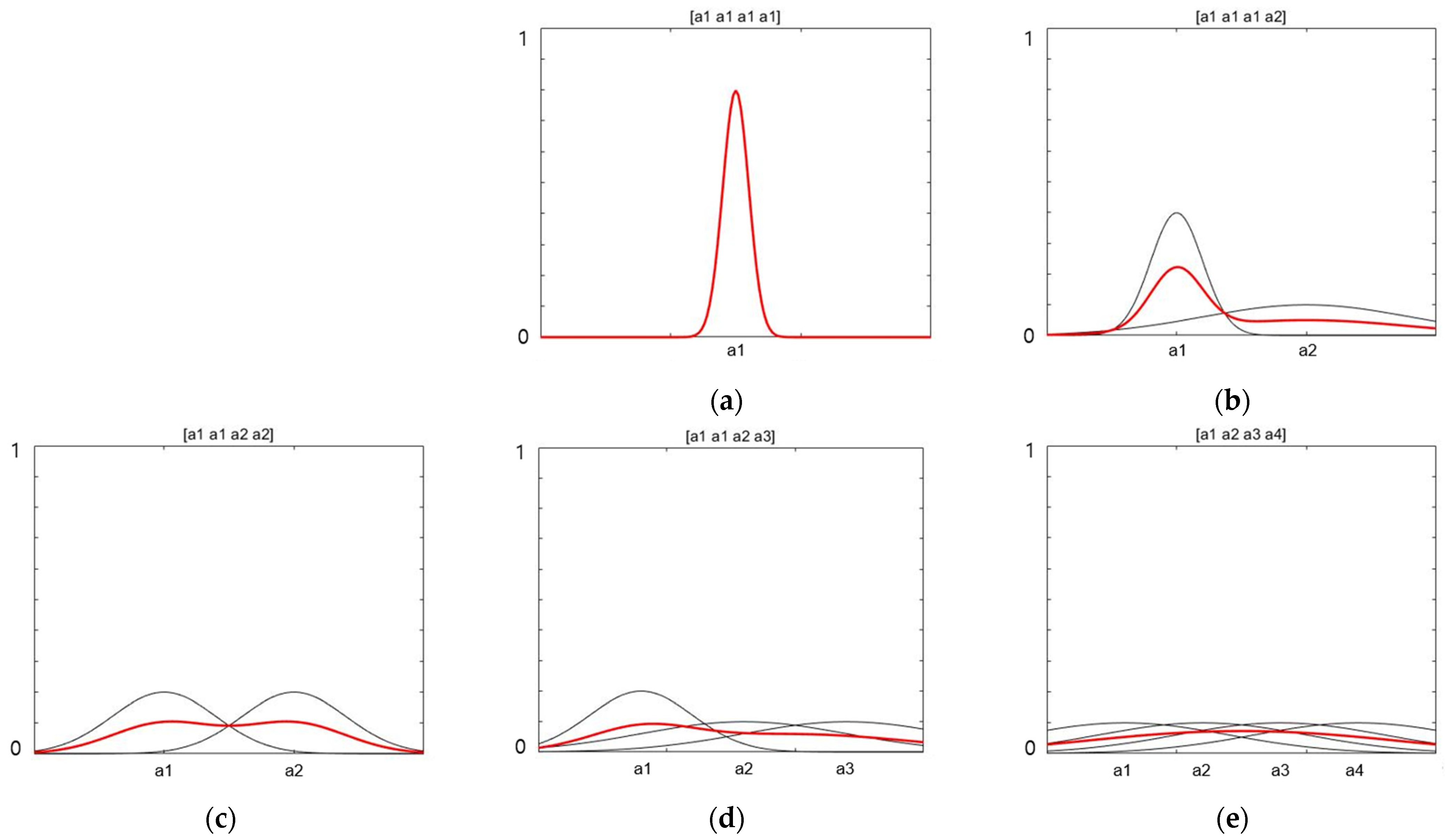
As illustrated in Figure 14, there were five cases where some of the four damage centers from the RMSE were determined as the same location of the damage center simultaneously, and the standard deviation for each case is shown in Table 4. The standard deviation was specified such that the maximum value from the probability function had a difference in multiples of two.
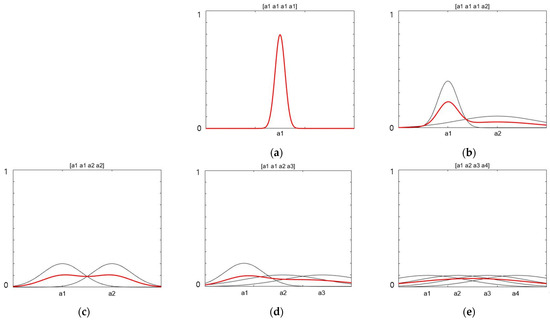
Figure 14.
Simplified combinations of probability functions: (a) [], (b) [], (c) [], (d) [], and (e) [].
Table 4.
Specified standard deviation for each number of repeated damage centers.
For the location of the damage center (a, b), which was predicted based on RMSE values, the probability function was applied in which the maximum probability existed at (a, b) in (x, z)-coordinates. The probability function was applied to all four predicted locations of the damage centers in one iteration if all the locations corresponded to different locations.
When some of the locations were repeated, a probability function was applied in which the maximum probability existed at the repeated point, and the standard deviation was determined according to Table 4. For example, when all four predicted locations of damage centers based on RMSE values indicated one location (, ) in (x, z)-coordinates, the probability function was applied in which the maximum probability existed at (, ), and the standard deviation was 0.5.
If there were more than one applied probability function, which means that two to four types of locations of the damage center were predicted, the average of all the function values at each coordinate point was calculated and became a final probability function. A combination of probability functions was available in five cases, and a simplified combination of cases of probability functions for explanation is shown in Figure 14. In the figure, the black line functions are the probability functions at each location of the damage centers, and the red line functions are the combined probability functions.
For example, [ ] in Figure 14b represents a situation where the three predicted damage centers are the same, except for one criterion. In this case, the final probability function values could be obtained by averaging the following two functions: a probability function with as its maximum probability point and a standard deviation of 1, and the probability function with as its maximum probability point and a standard deviation of 4.
The most adjacent integer point from the maximum probability point of the final probability function was selected as the predicted damage center for the iteration. For the following iterations, the final probability function values were stored and influenced future iterations by calculating the average, together with the new probability functions.
During sequential imports of the p-vector from the test datasets, the damage center could be confirmed when the same final predicted location was selected for five consecutive iterations. If all the iterations were consumed before five identical consecutive locations appeared, the mode location among all predicted locations became the confirmed location of the damage center for the test dataset.
For example, the changes in the probability function for the initial five iterations of the test dataset HS108HA030_SS04WA045 are shown in Figure 15. At the first iteration, location 108 was repeated for the pitch and total criteria; therefore, the surroundings of location 108 had a relatively high probability, and the most adjacent integer point from the maximum probability point was location 108. While the iterations progressed, location 108 was decided as the final predicted location of the damage center per iteration for the initial five iterations. Accordingly, location 108 was the confirmed predicted location of the damage center for the test dataset.
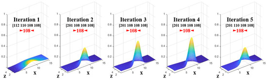
Figure 15.
Probability functions for the initial five iterations of the case HS108HA030_SS04WA045.
4. Results and Discussion
One hundred test datasets were randomly selected to predict the location of the damage center. The number of correct predictions (matches), the number of iterations required to confirm the location of the damage center, and the cases of incorrect predictions (mismatches) are listed in Table 5. For the mismatched cases, the correct location, which was the goal for the prediction, and the predicted location, which was the failed result of prediction, are shown as a three-digit number.
Table 5.
Test results using heave, roll, and pitch motions as criteria.
The correct damage center was found in 95 of the 100 test datasets, and in 71 cases, the damage center was confirmed within the initial five iterations.
Most digital inclinometers currently installed onboard only measure roll and pitch motions. Roll and pitch motion data and the sum of the RMSE for roll and pitch motions (excluding heave motion) were used to predict the damage center from the 100 randomly selected test datasets following the above procedure. The results are listed in Table 6.
Table 6.
Test results using only roll and pitch motions as criteria.
When using only roll and pitch motion data and their sum of the RMSE, 94 cases could predict the correct damage center, and among them, 81 cases confirmed the damage center within the initial five iterations. For three out of the six failed cases, the confirmed damage centers were adjacent. This indicates that although the heave motions were periodic, they did not have a significant effect on predicting the locations of damage centers through spectrum analysis.
Furthermore, the method spent 4.5 to 5.5 s per iteration. This indicates that the method was valid from the time perspective because it was developed under the assumption that real-time data are transmitted at intervals of 65 s at sea.
5. Conclusions
In this study, a method to predict the location of damage centers in ships using real-time ship motion data and a ship motion database was developed. Under different conditions, the simulated ship motion data were stored as a ship motion database and compared with real-time data to identify the location of the damage center.
Combinations of different locations of damage centers, sizes of the damaged area, sea states, and incident regular wave angles were used to simulate a total of 5400 cases in which the 6DOF motion data were obtained at intervals of 0.5 s for 60 min. The spectrogram matrices obtained by performing STFTs were used to construct the ship motion database. Then, 100 datasets were randomly selected, and a few initial raw data were removed to create the test datasets. The location of the damage center with the minimum RMSE value was selected based on the “heave,” “roll,” “pitch,” and “total” criteria. For the four predicted locations of damage centers based on the RMSE values of the x–z-coordinates, probability functions were applied. The location of the damage center with the highest probability was the confirmed predicted location of the damage center for each iteration of the test datasets. Similarly, the location of the damage center was predicted using only the roll and pitch motion data. The following conclusions were drawn from this study:
- In 95 out of 100 tests that used heave, roll, and pitch motion data, the location of the damage center was accurately predicted. Among these, 71 cases confirmed the damage center within the initial five iterations.
- When performing the same test using only roll and pitch motion data, the damage center was predicted correctly for 94 out of 100 tests. The results showed that the heave motions did not have a significant effect on predicting the location of the damage center using ship motion characteristics.
- Prediction of the damage center in this study took approximately 4.5 to 5.5 s per iteration, where real-time ship motion data collected for 130 s was used for each iteration of the prediction. Thus, the method is valid from a time perspective.
The proposed method could be used for existing ships as an alternative decision-making support method since some of them do not have sufficient flooding sensors. Furthermore, ships with flood sensors installed can use this method as additional information to the decision support system. While the proposed method does not require rapidly performable high computability, highly accurate results can be obtained, and applications to actual ships should be considered.
However, some challenges were faced during this study. Throughout this study, the flood accident situation within the predictable range was simulated and converted into a database, and the damage location was predicted. As a result, the validity of using the ship motion database was demonstrated. However, actual sea conditions are varying irregular waves. In the case of ships passing through certain seas, the simulation range can be reduced, but it is also not simple. Storing and inferring simulation results performed under more diverse conditions in a database and demonstrating the validity of the method could be a challenge for this method. Furthermore, after predicting the location of the damage center in the ship motion database, developing interpolation inference techniques to predict future accident situations or damage levels could be another challenge for this method.
Author Contributions
Conceptualization, H.-y.S. and S.-c.S.; methodology, H.-y.S. and H.-d.R.; software, H.-y.S., J.C. and D.-k.L.; validation, H.-y.S. and S.-j.O.; formal analysis, S.-j.O.; resources, J.C. and D.-k.L.; data curation, J.C. and D.-k.L.; writing—original draft preparation, H.-y.S.; writing—review and editing, H.-y.S. and G.-y.K.; visualization, H.-y.S.; supervision, S.-c.S.; project administration, S.-c.S. and G.-y.K.; funding acquisition, S.-c.S. All authors have read and agreed to the published version of the manuscript.
Funding
This research received no external funding.
Institutional Review Board Statement
Not applicable.
Informed Consent Statement
Not applicable.
Data Availability Statement
Not applicable.
Acknowledgments
This research was supported by the “Development of Autonomous Ship Technology (20200615)” funded by the Ministry of Oceans and Fisheries (MOF, Korea) and BK21 FOUR Graduate Program for Green-Smart Naval Architecture and Ocean Engineering of Pusan National University.
Conflicts of Interest
The authors declare no conflict of interest.
References
- Korea Maritime Safety Tribunal. Statistics of Marine Accidents [Marine Accidents by Accident Type] 2021. Available online: https://www.kmst.go.kr/eng/com/selectHtmlPage.do?htmlName=m4_vesseltype (accessed on 1 April 2021).
- Park, H.R.; Park, H.S.; Kim, B.R. A Study on the Policy Direction related to the Introduction of Maritime Autonomous Surface Ship (MASS); KMI Research Project Report; KMI: Pusan, Korea, 2018; No 2018-07. [Google Scholar]
- Lee, D.; Kim, S.; Lee, K.; Shin, S.C.; Choi, J.; Park, B.J.; Kang, H.J. Performance-based on-board damage control system for ships. Ocean Eng. 2021, 223, 108636. [Google Scholar] [CrossRef]
- Karolius, K.; Cichowicz, J.; Vassalos, D. Risk-Based Positioning of Flooding Sensors to Reduce Prediction Uncertainty of Damage Survivability. In Proceedings of the 13th International Conference on the Stability of Ships and Ocean Vehicles-STAB 2018, Kobe, Japan, 16–21 September 2018; pp. 627–637. [Google Scholar]
- Karolius, K.B.; Cichowicz, J.; Vassalos, D. Risk-based, sensor-fused detection of flooding casualties for emergency response. Ships Offshore Struct. 2021, 16, 449–478. [Google Scholar] [CrossRef]
- Varela, J.M.; Rodrigues, J.M.; Soares, C.G. On-board decision support system for ship flooding emergency response. Procedia Comput. Sci. 2014, 29, 1688–1700. [Google Scholar] [CrossRef] [Green Version]
- Varela, J.M.; Rodrigues, J.M.; Soares, C.G. 3D simulation of ship motions to support the planning of rescue operations on damaged ships. Procedia Comput. Sci. 2015, 51, 2397–2405. [Google Scholar] [CrossRef] [Green Version]
- Ruponen, P.; Lindroth, D.; Pennanen, P. Prediction of survivability for decision support in ship flooding emergency. In Proceedings of the 12th International Conference on the Stability of Ships and Ocean Vehicles STAB 2015, Glasgow, UK, 14–19 June 2015; pp. 14–19. [Google Scholar]
- Ruponen, P.; Pulkkinen, A.; Laaksonen, J. A method for breach assessment onboard a damaged passenger ship. Appl. Ocean Res. 2017, 64, 236–248. [Google Scholar] [CrossRef]
- Kang, H.; Choi, J.; Yim, G.; Ahn, H. Time Domain Decision-Making Support Based on Ship Behavior Monitoring and Flooding Simulation Database for On-Board Damage Control. In Proceedings of the 27th International Ocean and Polar Engineering Conference, San Francisco, CA, USA, 25–30 June 2017. [Google Scholar]
- Braidotti, L.; Mauro, F. A new calculation technique for onboard progressive flooding simulation. Ship Technol. Res. 2019, 66, 150–162. [Google Scholar] [CrossRef]
- Acanfora, M.; Begovic, E.; De Luca, F. A fast simulation method for damaged ship dynamics. J. Mar. Sci. Eng. 2019, 7, 111. [Google Scholar] [CrossRef] [Green Version]
- Braidotti, L.; Mauro, F. A fast algorithm for onboard progressive flooding simulation. J. Mar. Sci. Eng. 2020, 8, 369. [Google Scholar] [CrossRef]
- Papanikolaou, A.; Spanos, D. 24th ITTC benchmark study on numerical prediction of damage ship stability in waves preliminary analysis of results. In Proceedings of the 7th International Workshop on Stability and Operational Safety of Ships, Jiao Tong University, Shanghai, China, 1–3 November 2004. [Google Scholar]
- Ingale, R. Harmonic analysis using FFT and STFT. Int. J. Signal. Process. Image Process. Pattern Recognit. 2014, 7, 345–362. [Google Scholar] [CrossRef]
- Kehtarnavaz, N. Frequency Domain Processing. In Digital Signal Processing System Design; Elsevier: Amsterdam, The Netherlands, 2008; pp. 175–196. [Google Scholar]
- Boashash, B. Time-Frequency Signal Analysis and Processing: A Comprehensive Reference; Elsevier Science: Oxford, UK, 2015. [Google Scholar]
- Sairamya, N.J.; Susmitha, L.; George, S.T.; Subathra, M.S.P. Hybrid Approach for Classification of Electroencephalographic Signals Using Time–Frequency Images with Wavelets and Texture Features. In Intelligent Data Analysis for Biomedical Applications; Academic Press: Cambridge, MA, USA, 2019; pp. 253–273. [Google Scholar]
- Sugiyama, M. Examples of Continuous Probability Distributions. In Introduction to Statistical Machine Learning; Elsevier: Amsterdam, The Netherlands, 2015; pp. 37–50. [Google Scholar]
- Lee, G.J. Dynamic orifice flow model and compartment models for flooding simulation of a damaged ship. Ocean Eng. 2015, 109, 635–653. [Google Scholar] [CrossRef] [Green Version]
- IMO Res. MEPC.110(49), Revised Interim Guidelines for the Approval of Alternative Methods of Design and Construction of Oil Tankers under Regulation 13F(5) of Annex I of MARPOL 73/78). Available online: http://rise.odessa.ua/texts/MEPC110_49e.php3 (accessed on 24 October 2021).
- Rules for Classification: Ships—DNVGL-RU-SHIP, Pt.3 Ch.15. Edition July 2016, Amended January 2017, Stability. Available online: https://rules.dnv.com/docs/pdf/DNV/ru-ship/2017-01/DNVGL-RU-SHIP-Pt3Ch15.pdf (accessed on 26 October 2021).
- Jin, S.M. Introduction to the Spectrum and Spectrogram. J. Korean Soc. Laryngol. Phoniatr. Logop. 2008, 19, 101–106. [Google Scholar]
- Gautam, G.; Shrestha, S.; Cho, S. Spectral Analysis of Rectangular, Hanning, Hamming and Kaiser Window for Digital Fir Filter. Int. J. Adv. Smart Converg. 2015, 4, 138–144. [Google Scholar] [CrossRef] [Green Version]


Publisher’s Note: MDPI stays neutral with regard to jurisdictional claims in published maps and institutional affiliations. |
© 2021 by the authors. Licensee MDPI, Basel, Switzerland. This article is an open access article distributed under the terms and conditions of the Creative Commons Attribution (CC BY) license (https://creativecommons.org/licenses/by/4.0/).