Fatigue Assessment of Moorings for Floating Offshore Wind Turbines by Advanced Spectral Analysis Methods

Abstract

The fatigue assessment of mooring lines for floating offshore wind turbines represents a challenging issue not only for the reliable design of the stationkeeping system but also for the economic impact on the installation and maintenance costs over the entire lifetime of the offshore wind farm. After a brief review about the state-of-art, the nonlinear time-domain hydrodynamic model of floating offshore wind turbines moored by chain cables is discussed. Subsequently, the assessment of the fatigue damage in the mooring lines is outlined, focusing on the combined-spectrum approach. The relevant fatigue parameters, due to the low- and wave-frequency components of the stress process, are estimated by two different methods. The former is based on the time-domain analysis of the filtered stress process time history. The latter, instead, is based on the spectral analysis of the stress process by two advanced methods, namely the Welch and Thomson ones. Subsequently, a benchmark study is performed, assuming as reference floating offshore wind turbine the OC4-DeepCWind semisubmersible platform, equipped with the 5 MW NREL wind turbine. The cumulative fatigue damage is determined for eight load conditions, including both power production and parked wind turbine situations. A comparative analysis between time-domain and spectral analysis methods is also performed. Current results clearly show that the endorsement of advanced spectral analysis methods can be helpful to improve the reliability of the fatigue life assessment of mooring lines.

1. Introduction

The reliability of long-term mooring systems for floating offshore wind turbines (FOWTs), deployed on intermediate and deep-water depth, is a key factor to move the offshore wind energy sector towards the commercialization phase, provided that in the last two decades several accidents, mainly due to mooring failures, occurred throughout the world [1]. Indeed, one of the expected goals of the Horizon 2020 “Secure, clean and efficient energy” work programme [2] is the development of reliable, sustainable and cost-efficient mooring systems for FOWTs, with the main aim of making the offshore wind energy sector more competitive on the international market, as regards other well-established renewable sources.

As previously said, the need of further improving the hydrodynamic modelling of FOWTs, as well as the design of long-term moorings, is due to the high number of failure events that occurred in the last decade, as stressed by Kvitrud [3], among others, who reported 15 mooring failures in the Norwegian sea area during the years 2010–2013, one-third of which were due to single or multiple fatigue failures of mooring lines. Starting from the pioneering research by de Laval [4] and van Helvoirt [5], who performed the first fatigue tests on mooring chains at the beginning of 1970s and 1980s, respectively, the fatigue analysis of mooring lines quickly became a very popular topic, following the growth of the oil and gas industry, the need of exploiting subsea oilfields and the increasing demand for floating offshore structures to be deployed on deep-water depths. Past research activities focused on a variety of topics involved in the fatigue analysis of mooring systems, among which were the following: the simultaneous presence of low- and wave-frequency components in the mooring line stress process [6], the occurrence of bimodal non-Gaussian random processes [7], the application of spectral analysis and rainflow counting methods for the fatigue analysis of mooring lines [8].

More recently, following the increasing demand for energy from renewable sources and the rapid development of the offshore wind technology, attention was also paid to the design and analysis of stationkeeping systems for FOWTs deployed on intermediate and deep-water depths. Most of past research activities in this field focused on the design and optimization of mooring systems, with the main aim of reducing the installation costs of wind farms and making the offshore wind energy sector more competitive on the international market, in terms of the levelized cost of energy. Particularly, Brommundt et al. [9] provided a frequency-domain tool for the optimization of mooring systems and applied it to a reference semisubmersible tri-floater support structure deployed on two different water depths, namely 75 and 330 m. Benassai et al. [10,11] carried out a benchmark study, devoted to investigating the incidence of the main design parameters, namely the number and type of mooring lines, on the total weight of the stationkeeping system at different water depths. Kim et al. [12] designed the stationkeeping system for an FOWT, deployed in the Jeju offshore basin. Hall and Goupee [13] introduced a lumped-mass mooring line model for FOWTs and validated it against a set of experimental tests on a tri-floater platform. Campanile et al. [14] focused on the design of mooring systems for FOWTs to be deployed on intermediate water depths and furnished some suggestions to reduce the weight of the stationkeeping system from the preliminary design phase.

Following this brief review about the state-of-art concerning the analysis of mooring systems for FOWTs, only few attempts were devoted to the fatigue analysis of mooring lines, as most of past research focused on the ultimate and accidental limit state design conditions for stationkeeping systems [10,11,12,13,14]. Really, the assessment of the fatigue damage in the mooring lines of FOWTs still presents some challenging issues, mainly related to the combined presence of both low- and wave-frequency stress components that, in turn, need to be separately evaluated to assess the cumulative fatigue damage in the mooring line. In this respect, the actual rules and guidelines for the design of stationkeeping systems [15] suggest the employment of the combined-spectrum approach when bimodal stress processes are expected to occur. Nevertheless, one of the main issues that arise when this method is applied is mainly due to the assessment of the low- and wave-frequency components, starting from the time history of the combined stress process. In this respect, starting from the pioneering work by Winterstein [16] in 1988, some years later Jiao and Moan [17] developed the so-called dual narrow-band method for the assessment of the fatigue damage for bimodal stress processes and this is still embodied in current rules and guidelines for the design and analysis of mooring systems [15]. In the following years, several spectral methods were developed to improve the accuracy of the fatigue assessment [18,19], when both low- and high-frequency components occur. In the last decade, improved methods were developed for bimodal Gaussian [20,21,22] and non-Gaussian processes [23,24,25,26,27,28], with the main aim of improving the accuracy of the fatigue damage assessment.

Hence, in the current analysis, a time-domain method, based on the application of low-pass and high-pass filters to the initial stress process, is compared with two advanced spectral analysis techniques, based on the Welch and Thomson methods, with the main aim of investigating the incidence of the use of time- and frequency-domain analyses on the assessment of cumulative fatigue damage in the mooring lines. This issue is worthy of investigation not only because the stress process in the mooring lines is generally bimodal but also because the low-frequency component consists of two different contributions, due to the slowly varying drift forces and the turbulent component of the wind loads acting on the emerged part of the support structure and the wind turbine. The paper is structured as follows. Section 2 provides a brief review of the nonlinear time-domain hydrodynamic and mooring models. Section 3 focuses on the fatigue analysis of mooring lines by the combined-spectrum approach. Section 4 discusses the Welch and Thomson methods, applied in the benchmark study. Section 5 provides the main data of the reference FOWT, as well as the basic load conditions, involving both power production and parked wind turbine situations that are analysed in Section 6. Finally, Section 7 and Section 8 provide the discussion of the main outcomes gathered by the benchmark study and the conclusions. All calculations were performed by a set of dedicated codes developed in MATLAB.

2. Model Description of Dynamic Analysis

The reference tri-floater support structure, assumed in the subsequent benchmark study, is the OC4-DeepCWind platform [29], equipped with the 5 MW NREL wind turbine [30]. It is equipped with three mooring lines, spread 120° apart, as depicted in Figure 1.

The nonlinear time-domain motion equations, as regards the global reference system with origin on the projection of the FOWT centre of mass on the waterplane area, are provided by Equation (1), which represents the commonly embodied hydrodynamic model for FOWTs [31,32,33]:

$$\left(\mathit{M}+{\mathit{A}}_{\infty }\right)\ddot{\mathit{q}}+{\int }_{-\infty }^t\mathit{R}\left(t-\tau \right)\dot{\mathit{q}}\left(\tau \right)d\tau +\mathit{K}\mathit{q}={\mathit{F}}_{\mathit{w}\mathit{a}\mathit{v}\mathit{e}}\left(t\right)+{\mathit{F}}_{\mathit{w}\mathit{i}\mathit{n}\mathit{d}}\left(t\right)+{\mathit{F}}_{\mathit{v}\mathit{i}\mathit{s}\mathit{c}}\left(t\right)+{\mathit{F}}_{\mathit{m}\mathit{o}\mathit{o}\mathit{r}}\left(t\right)$$

(1)

where $\mathit{M}$ is the mass matrix; ${\mathit{A}}_{\infty }$ is the added mass matrix at infinite frequency; $\ddot{\mathit{q}}$, $\dot{\mathit{q}}$ and $\mathit{q}$ are the 6DOF acceleration, velocity and displacement vectors; $\mathit{R}$ is the retardation function matrix; ${\mathit{F}}_{\mathit{w}\mathit{a}\mathit{v}\mathit{e}}$ is the vector of first- and second-order wave excitation forces; ${\mathit{F}}_{\mathit{w}\mathit{i}\mathit{n}\mathit{d}}$ is the wind force vector, including both steady and turbulent components; ${\mathit{F}}_{\mathit{v}\mathit{i}\mathit{s}\mathit{c}}$ is the drag force vector and ${\mathit{F}}_{\mathit{m}\mathit{o}\mathit{o}\mathit{r}}$ is the mooring force vector. The retardation function matrix is determined by the inverse Fourier transform of the frequency-dependent linear radiation damping matrix $\mathit{B}$, according to Equation (2), which is based on the Cummins [34] approach:

$$\mathit{R}\left(t\right)=\frac{2}{\pi }{\int }_0^{\infty }\mathit{B}\left(\omega \right)cos\left(\omega t\right)d\omega$$

(2)

where $\omega$ denotes the wave circular frequency. Wave forces include both first- and second-order components. The former was randomly generated using Equation (3):

$${\mathit{F}}_{\mathit{w}\mathit{a}\mathit{v}\mathit{e}}^{\left(\mathit{I}\right)}\left(t\right)=Re{{\displaystyle \sum }}_{j=1}^N{A}_j{\mathit{X}}^{\left(\mathit{I}\right)}\left({\omega }_j,{\beta }_j\right)e^{i{\omega }_{j}t}$$

(3)

where $A_j$ is the magnitude of a regular incident wave with circular frequency ${\omega }_j$ and direction ${\beta }_j$, while ${\mathit{X}}^{\left(\mathit{I}\right)}$ is the vector of the first-order complex excitation transfer function, corresponding to the circular frequency ${\omega }_j$ and direction ${\beta }_j$. As concerns the second-order wave forces, they include both difference- and sum-frequency components among pairs of incoming waves [31]. Nevertheless, in the current analysis, only the difference-frequency components, namely the so-called slowly varying drift forces, were considered, according to Equation (4):

$${\mathit{F}}_{\mathit{w}\mathit{a}\mathit{v}\mathit{e}}^{\left(\mathit{I}\mathit{I}\right)}\left(t\right)=Re{{\displaystyle \sum }}_{j=1}^N{{\displaystyle \sum }}_{k=1}^N{A}_j{A}_k^{*}D\left({\omega }_j,{\omega }_k\right)e^{i\left({\omega }_j-{\omega }_k\right)t}{\mathit{h}}_{\mathit{w}}$$

(4)

where the asterisk (*) denotes the complex conjugate operator; ${\mathit{h}}_{\mathit{w}}$ is the wave direction vector and $D$ is the difference-frequency quadratic transfer function (QTF) at the pair of frequencies ${\omega }_j$ and ${\omega }_k$ that, in turn, is assessed by the far-field approach [35]. The magnitude of each wave component was determined using Equation (5):

$$A_j=\sqrt{S\left({\omega }_j\right)\Delta \omega }$$

(5)

where $S$ is the wave spectrum and $\Delta \omega$ is the wave frequency interval, to be selected less than $2\pi /T$ to ensure the randomness of simulation in the time interval $T$.

The wind loads acting on the emerged part of the tri-floater support structure and wind turbine were determined by using Equation (6):

$${\mathit{F}}_{\mathit{w}\mathit{i}\mathit{n}\mathit{d}}\left(t\right)=\frac{1}{2}{\rho }_{a}A{C}_{d,w}{v}_w^2{\mathit{h}}_{\mathit{w}\mathit{i}\mathit{n}\mathit{d}}$$

(6)

where ${\rho }_a$ is the standard air density; $A$ is the structural element projected area normal to the wind direction; $C_{d,w}$ is the drag coefficient; ${\mathit{h}}_{\mathit{w}\mathit{i}\mathit{n}\mathit{d}}$ is the wind direction vector and $v_w$ is the wind relative velocity, consisting of both steady and turbulent components, the latter generated according to the Norwegian Petroleum Directorate wind spectrum [36]. A similar approach was followed to assess the force exerted by the wind turbine, after replacing the drag coefficient $C_d$ by the relevant thrust coefficient $C_t$, depending on the wind speed at hub height [37]. This approach is certainly slightly approximate, as regards well-established and more refined techniques, mainly based on the blade element momentum (BEM) theory [38], but it is accurate enough for the fatigue life assessment of mooring lines, as proved by the benchmark study recently carried out by Barrera et al. [32] on the OC4-DeepCwind platform.

The viscous forces acting on the submerged part of the tri-floater support structure were determined according to the Morison equation and the relative velocity formulation [39] using Equation (7):

$${\mathit{F}}_{\mathit{v}\mathit{i}\mathit{s}\mathit{c}}\left(t\right)=\frac{1}{2}{\rho }_{w}A{C}_{d,v}\left[u\left(t\right)-\dot{\mathit{q}}\left(t\right)·{\mathit{h}}_{\mathit{w}}\right]\left|u\left(t\right)-\dot{\mathit{q}}\left(t\right)·{\mathit{h}}_{\mathit{w}}\right|{\mathit{h}}_{\mathit{w}}$$

(7)

where ${\rho }_w$ is the standard water density, $u$ is the wave particle velocity and $C_{d,v}$ is the drag coefficient. The same notation, already endorsed for wind forces, was also applied for the remaining physical quantities.

The quasi-static equilibrium model was applied to evaluate the nonlinear mooring forces, considering the seabed friction, the nonlinear restoring components and the line stiffness. Both inertia and damping forces, exerted by the mooring lines, were neglected in this study with no appreciable errors. Really, the validity of this assumption mainly depends on the weight of the mooring system relative to the weight of the floating platform. From a general point of view, if the inertia and damping forces exerted by the stationkeeping system are neglected, some appreciable errors in the assessment of the mooring line forces may arise [13]. Anyway, if the weight of the mooring system is low in comparison with that of the floating platform, the quasi-static model does not significantly affect the hydrodynamics of the FOWT [40] and the fatigue life assessment. This outcome was recently stressed by Trubat et al. [41], who investigated the incidence of the mooring hydrodynamics on the assessment of mooring line tension and fatigue for the stationkeeping system of the OC5-DeepCWind platform, verifying that almost the same values were obtained without and with the above-mentioned components. The horizontal, $H_F,$ and vertical, $V_F,$ forces at the fairlead of each mooring line were determined according to a local reference system, having origin at the anchoring point, according to the nonlinear implicit equation systems (8a) and (8b) for fully and partly developed catenary configurations, respectively:

$$\begin{array}{l}{x}_F=\frac{H_F}{w}\left\{ln\left[\frac{V_F}{H_F}+\sqrt{1+{\left(\frac{V_F}{H_F}\right)}^2}\right]-ln\left[\frac{V_F-wL}{H_F}+\sqrt{1+{\left(\frac{V_F-wL}{H_F}\right)}^2}\right]\right\}+\frac{H_{F}L}{E{A}_c}\hfill \\ z_F=\frac{H_F}{w}\left[\sqrt{1+{\left(\frac{V_F}{H_F}\right)}^2}-\sqrt{1+{\left(\frac{V_F-wL}{H_F}\right)}^2}\right]+\frac{1}{E{A}_c}\left(V_{F}L-\frac{w{L}^2}{2}\right)\hfill \end{array}$$

(8a)

$$\{\begin{array}{l}{x}_F=L_b+\frac{H_F}{w}ln\left[\frac{V_F}{H_F}+\sqrt{1+{\left(\frac{V_F}{H_F}\right)}^2}\right]+\frac{H_{F}L}{E{A}_c}+\frac{c_{b}w}{2E{A}_c}\left[-L_b{}^2+\left(L_b-\frac{H_F}{c_{b}w}\right)max\left\{L_b-\frac{H_F}{c_{b}w};0\right\}\right]\hfill \\ z_F=\frac{H_F}{w}\left[\sqrt{1+{\left(\frac{V_F}{H_F}\right)}^2}-\sqrt{1+{\left(\frac{V_F-wL}{H_F}\right)}^2}\right]+\frac{1}{E{A}_c}\left(V_F{L}_c-\frac{w{L}^2}{2}\right)\hfill \end{array}$$

(8b)

In Equations (8a) and (8b), $x_F \left(z_F\right)$ is the fairlead horizontal (vertical) coordinate, as regards the local reference system; $w$ is the mooring line unit weight in water; $L$ is the line length; $E$ ($A_c$) is the line Young modulus (cross-section); $L_b=L-V_F/w$ is the line length lying on the seabed and $c_b$ is the bottom drag coefficient. The mooring force equations were preliminarily solved by the Newton–Raphson iteration scheme [42] and subsequently resembled into the global reference system.

The equation system (1) was solved by a dedicated programme developed in MATLAB [43], by the ode45 solver, after determining an approximate 10th-order state-space realization of each convolution integral [44] by the Hankel singular-value decomposition algorithm [45]. Finally, the frequency-dependent added masses, radiation dampings and normalized wave excitation forces were determined by the open-source code NEMOH [46].

3. Fatigue Analysis of Mooring Lines

3.1. The Combined-Spectrum Approach

Mooring lines are subjected to random cyclic loadings during the entire lifetime that significantly affect the fatigue life of the stationkeeping system. Under irregular cyclic loadings, the fatigue analysis of mooring lines is generally performed according to the Miner rule [47], and the accumulated fatigue damage, $d,$ is determined by Equation (9):

$$d={\displaystyle \sum }_{j=1}^N\frac{n_j}{N_j}$$

(9)

where $n_j$ is the number of cycles, associated with a certain stress range ${\sigma }_j$, and $N_j$ is the maximum allowable number of cycles, which, in turn, is determined by Equation (10):

$$N_j=K{\sigma }_j^{-m}$$

(10)

where $K$ and $m$ are the intercept and slope parameters of the mooring line S–N curve, whose values are listed in the following with reference to stud-link chain cables. Nevertheless, when the stress history in the mooring line is random, as typically occurs in a seaway, the cumulative fatigue damage needs to be replaced by the relevant expected value [19,48]. In this respect, if the stress history is a Gaussian narrow-band process, the stress range follows the Rayleigh distribution, so that the expected fatigue damage, $\overline{d,}$ is determined by Equation (11):

$$\overline{d}={\displaystyle \sum }_{j=1}^N\frac{{\nu }_j{T}_j}{K}{\left(2\sqrt{2}{\sigma }_j\right)}^m\mathsf{\Gamma }\left(1+\frac{m}{2}\right)$$

(11)

where ${\nu }_j$ and ${\sigma }_j$ are the zero up-crossing frequency and the standard deviation of the random j-th stress process, respectively; $T_j$ is the exposure time to the j-th sea state condition and $\mathsf{\Gamma }$ is the Gamma function. The previous approach is valid for unimodal stress processes, and so it needs to be properly modified if the stress history is bimodal, as generally occurs for FOWTs. In this case, the low-frequency components, due to the slowly varying drift forces and the turbulent component of wind loads, arise in addition to the wave-frequency stress process, due to first-order wave forces. In this respect, there is a wide consensus that the rainflow method provides the best estimate of the cumulative fatigue damage for bimodal stress processes, but it is very time-consuming [49]; therefore, it is generally replaced by the combined-spectrum approach. Hence, the expected cumulative fatigue damage was assessed by Equation (11), after applying the replacements provided by Equation (12):

$${\sigma }_j=\sqrt{{\sigma }_{j,L}^2+{\sigma }_{j,W}^2} ; {\nu }_j=\sqrt{{\left(\frac{{\sigma }_{j,L}}{{\sigma }_j}{\nu }_{j,L}\right)}^2+{\left(\frac{{\sigma }_{j,W}}{{\sigma }_j}{\nu }_{j,W}\right)}^2}$$

(12)

where ${\sigma }_{j,L}$ $({\sigma }_{j,W})$ and ${\nu }_{j,L}$ $({\nu }_{j,W})$ are the standard deviation and the zero up-crossing rate of the j-th low-frequency (wave-frequency) stress process. This approach, which is based on the simple summation of two narrow-band Gaussian stress processes, provides a conservative estimate of the cumulative fatigue damage if bimodal conditions occur. The validity of the assumption about the Gaussianity of the stress process is further discussed in Appendix A. As concerns the second assumption, the fatigue damage was assessed by the combined-spectrum approach, based on Equations (11) and (12), assuming that the low- and wave-frequency components of the stress process were narrow-banded. Really, this assumption is on the safe side, as it furnishes a slight conservative estimate of the cumulative fatigue damage in the mooring lines. In addition, it does not affect the main findings of the benchmark study, provided that the cumulative fatigue damage is always obtained by the combined-spectrum approach, after determining the main input parameters by time-history or spectral analysis, as further discussed in Section 3.2 and Section 3.3.

3.2. Fatigue Assessment by Time-History Analysis

One of the main issues, arising from the application of the combined-spectrum approach, is mainly related to the assessment of the standard deviation and zero up-crossing rates of the low- and wave-frequency components of the stress process. A method, that can be easily implemented to evaluate the above-mentioned quantities, is the signal filtering of the stress process time history. In this respect, the time histories of the low- (wave-) frequency component of the stress process can be detected, after applying an infinite impulse response low-pass (high-pass) filter to the initial random signal [43], with a proper passband frequency and impulse steepness. The passband frequency, $\widehat{f}$, is generally set depending on the typical periods of the low- and wave-frequency components of the stress process. The impulse steepness, $s$, instead, is related to the width of the transition region interested by low-pass $\Delta f_L$ and high-pass $\Delta f_H$ filters, according to Equation (13):

$$\Delta f_L=\left(1-s\right)\left(f_{Ny}-\widehat{f}\right) ; \Delta f_H=\left(1-s\right)\widehat{f}$$

(13)

where $f_{Ny}$ is the Nyquist frequency. This method is very effective and less time-consuming, but the selection of the passband frequency and impulse steepness is a key factor for the assessment of the low- and wave-frequency components of the stress process. In the current analysis, the passband frequency, $\widehat{f},$ was set equal to 0.05 Hz and impulse steepness was assumed to be equal to 0.99. The passband frequency corresponded to a period of 20 s, which is a reasonable upper bound for typical waves in open sea conditions. The impulse steepness, instead, was selected high enough to ensure a good separation between the low- and high-frequency contents of the stress signal. The reliability of these assumptions was implicitly checked by the comparative analysis outlined in Section 7. After separately detecting the time histories of the low- and wave-frequency components, the relevant standard deviations were immediately determined. Instead, the zero up-crossing rates, ${\nu }_{j,L}$ and ${\nu }_{j,W},$ were estimated using Equation (14):

$${\nu }_{j,L}=\frac{1}{T_n} ; {\nu }_{j,W}=\frac{1}{T_p}$$

(14)

where $T_n$ is the surge natural period of the FOWT and $T_p$ is the wave peak period of the first-order wave forces. The effectiveness of these two assumptions was checked by comparative analysis with the advanced spectral analysis methods outlined in Section 4.

3.3. Fatigue Assessment by Spectral Analysis

The cumulative fatigue damage in the mooring lines can be also determined by spectral analysis, after determining the bimodal spectrum of the stress process, $S_{\sigma }\left(f\right),$ by the advanced spectral analysis techniques outlined in Section 4. Once the combined spectrum was determined and the separation frequency, $\widehat{f},$ was selected, the spectra of low- and wave-frequency components were determined using Equation (15):

$$S_{\sigma ,L}\left(f\right)=\{\begin{array}{l}{S}_{\sigma }\left(f\right) if f\le \widehat{f} \hfill \\ 0 otherwise\hfill \end{array};S_{\sigma ,W}\left(f\right)=\{\begin{array}{l}{S}_{\sigma }\left(f\right) if f>\widehat{f} \hfill \\ 0 otherwise\hfill \end{array}$$

(15)

which implies that the two spectra are non-overlapping and the equality provided by Equation (16) holds:

$$S_{\sigma }\left(f\right)=S_{\sigma ,L}\left(f\right)+S_{\sigma ,W}\left(f\right)$$

(16)

The standard deviation of the low- and wave-frequency stress processes was directly determined by the zero-order spectral moments of the low- and wave-frequency spectra, according to Equation (17):

$${\sigma }_{j,L}={{\displaystyle \int }}_0^{\widehat{f}}{S}_{\sigma }\left(f\right)df;{\sigma }_{j,W}={{\displaystyle \int }}_{\widehat{f}}^{\infty }{S}_{\sigma }\left(f\right)df$$

(17)

while the zero up-crossing rates were assessed using Equation (18), depending on the zero- and second-order spectral moments:

$${\nu }_{j,L}=\sqrt{\frac{{{\displaystyle \int }}_0^{\widehat{f}}{f}^2{S}_{\sigma }\left(f\right)df}{{{\displaystyle \int }}_0^{\widehat{f}}{S}_{\sigma }\left(f\right)df}};{\nu }_{j,W}=\sqrt{\frac{{{\displaystyle \int }}_{\widehat{f}}^{\infty }{f}^2{S}_{\sigma }\left(f\right)df}{{{\displaystyle \int }}_{\widehat{f}}^{\widehat{\infty }}{S}_{\sigma }\left(f\right)df}}$$

(18)

This procedure allows the easy detection of all fatigue parameters required to apply the combined-spectrum method, once the spectrum of the combined stress process, $S_{\sigma },$ is detected, as discussed in Section 4.

4. Advanced Spectral Analysis

4.1. Welch Method

Spectrum estimation methods include two main groups, namely nonparametrical and parametrical [50]. The former are based on the application of the Fourier transform (FT) to data, together with proper pre-processing and, eventually, averaging operations. The latter are based on fitting flexible models to the data, such the auto-regressive (AR) or the auto-regressing moving average (ARMA) ones, and then obtaining analytically the corresponding power spectrum. In this paper, two main nonparametrical methods were investigated, namely the Welch’s overlapped segment averaging (WOSA) and Thomson multi-taper method (MTM), leaving the examination of the nonparametrical approach to a possible future development [51].

The Welch method consists in parsing the data record, corresponding to an overall observation duration, $T$, in smaller segments of duration $T_0$, with partial overlap, typically from 20% to 50%. Each segment was pre-treated by tapering with a smooth window, to reduce the bias due to spectral leakage, then the “periodogram”, i.e., the square of the FT of the series of observations, normalized in respect to the duration $T_0$, was calculated for each of them. The spectrum was obtained by averaging over such periodograms. This combination of data tapering and averaging provides a reduction of bias due to spectral leakage and variance related to the randomness of the process [52].

To get some insight in the corresponding estimation procedure, let us denote the series of observations by $x_i=x\left(i\Delta t\right)$, where $\Delta t$ is the sampling interval, and $i=1,\dots N$, with $T=N\Delta t$, and $T_0=N_0\Delta t$. Let $w_1,\dots ,w_{N_0}$ be a data taper, then the modified periodogram for the $l$-th segment is given as follows:

$${\widehat{S}}_l\left(f\right)=\Delta t{\left|{\displaystyle \sum }_{i=1}^{N_0}{w}_i{x}_{i+l-1}{e}^{-j2\pi fi\Delta t}\right|}^2$$

(19)

where $j$ is the imaginary unit. The spectral estimator is then:

$$\widehat{S}\left(f\right)=\frac{1}{n}{\displaystyle \sum }_{k=0}^{n-1}{\widehat{S}}_{km+1}\left(f\right)$$

(20)

where $n$ is the number of segments and $m$ is an integer-valued shift factor, satisfying $0<m\le N_0$ and $m\left(n-1\right)=N-N_0$.

To optimize the performance of the analyser, two main conflicting features, namely the “effective bandwidth” and the variance (or, equivalently, the standard deviation), have to be controlled to achieve an optimum trade-off. The effective bandwidth is a measure of the minimum separation in frequency between approximately uncorrelated spectral estimates: thus, the wider such bandwidth is, the worse spectral resolution is. For Welch’s method, it can be expressed as $\Delta f_e={\alpha }_w{T}_0^{-1},$ where ${\alpha }_w$ is a factor that depends upon the kind of the selected taper and on the way bandwidth is defined. In the case of the Hanning window and considering a half-power bandwidth, we obtain ${\alpha }_w=1.44$. On the other hand, standard deviation of the estimator is a measure of its uncertainty, for a given effective bandwidth. For the Welch method, with a 50% overlap, a relative standard uncertainty (standard deviation) $u_S\left(f\right)/S\left(f\right)=\sqrt{\left(11/18\right)N_0{N}^{-1}}$ can be assumed, where $u_S\left(f\right)$ is the absolute standard uncertainty. Once the record duration $T$ is fixed and the kind of taper and the degree of overlap have been decided, the duration of the observation window, $T_0$, remains the only design parameter to be optimized, with a trade-off between the need to have a good spectral resolution, which demands a large $T_0$, and a small standard uncertainty, which requires a small $T_0.$

4.2. Thomson Method

This method generalizes the tapering issue by adopting multiple orthogonal tapers to recover the information that may be lost when using a single taper. The estimator is the average of $K$ direct spectral estimators, each acting on the whole data record (rather than on a signal segment, as happens in Welch method) and applying a different taper. Each partial estimator is defined by

$${\widehat{S}}_k\left(f\right)=\Delta t{\left|{\displaystyle \sum }_{i=1}^N{h}_{i,k}{x}_{i+l-1}{e}^{-j2\pi fi\Delta t}\right|}^2$$

(21)

where $h_{i,k}$ is the $k$th data taper, usually chosen as the $k$th discrete prolate spheroidal sequence with parameter $W$, where $2W$ is the normalized bandwidth of the tapers, i.e., the bandwidth for $\Delta t=1\mathrm{s}$. The final estimator is thus as follows:

$$\widehat{S}\left(f\right)=\frac{1}{K}{\displaystyle \sum }_{k=0}^{K-1}{\widehat{S}}_k\left(f\right)$$

(22)

where $K$ is typically chosen to be equal to $2NW-1$ [53].

Again, a trade-off is required between effective bandwidth and relative standard uncertainty. The effective bandwidth can be estimated as $\Delta f_e=2W/\Delta t$ (Hz). Furthermore, considering that the distribution of the estimator can be approximated by $S\left(f\right){\chi }_{2K}^2/2K$, the relative standard uncertainty was equal to $K^{-\frac{1}{2}}$. There is here much less arbitrariness than in Welch’s method, since, for a fixed observation time, $T$, the only parameter to be chosen was the half-bandwidth $W$, which influences both spectral resolution and relative standard uncertainty.

5. Main Input Data

5.1. The OC4-DeepCwind Platform

The OC4-DeepCwind platform [29] consists of a tri-floater support structure, equipped with the NREL 5 MW wind turbine [30]. It has three offset columns, connected to each other by two sets of bracings and consisting of an upper and a base cylinder, the latter with an enlarged diameter to suppress, as far as possible, the heave motion of the FOWT. The tri-floater is also equipped with a central main column that supports the tower of the wind turbine and is connected to the offset columns by an additional set of bracings. The main properties of the FOWT are listed in

Table 1. Main properties of the OC4-DeepCwind platform.

Total platform draught	20.0 m
Elevation of tower base/hub height above SWL	10.0/90.0 m
Diameter of bracings/main column	1.6/6.50 m
Diameter of upper columns/base columns	12.0/24.0 m
Height of upper columns/base columns	26.0/6.0 m
Spacing between offset columns	50.0 m
Platform displacement	14,070 t
Cut-in/rated/cut-out wind speed at hub height	3.0/11.4/25.0 m/s
Rotor/hub diameter	126.0/3.0 m
Vertical coordinate of the centre of mass/centre of buoyancy as regards the SWL	−9.94/−13.23 m
Roll–pitch/yaw moment of inertia as regards the centre of mass	1.10 × 107/1.23 × 107 tm2
Surge–sway/heave added mass at infinite frequency	6440/14,500 t
Roll–pitch/yaw added mass at infinite frequency	7.17 × 106/4.90 × 106 tm2
Heave restoring coefficient	3411 t/s2
Roll–pitch restoring coefficient	1.028 × 106 tm2/s2
Surge/sway natural period	116 s
Drag coefficient of the submerged part of main/offset columns (viscous forces)	0.56/0.61
Drag coefficient of base columns (viscous forces)	0.68
Drag coefficient of the emerged part of main/offset columns (wind forces)	0.42
Drag coefficient of the turbine tower (wind forces)	0.59

, while the thrust curve of the wind turbine is provided in Figure 2, as a function of the wind speed at hub height, for both power production and parked wind turbine conditions [37,54]. In this respect, it must be pointed out that the rotor control mechanism of the wind turbine was not considered here. Anyway, it is expected that this assumption does not significantly affect the analysis performed in Section 6. In fact, Barrera et al. [32] recently carried out a comparative analysis on the stress histories in the mooring lines of the OC4-DeepCWind platform, modelling the wind forces by a look-up table of thrust coefficients and by the blade element momentum theory, including, in the latter case, the rotor control mechanism of the wind turbine. They verified that the agreement between the different numerical approaches and the experimental results was always very good. The response amplitude operators (RAOs) due to first-order wave loads and the second-order difference-frequency quadratic transfer functions (QTFs) of the OC4-DeepCWind platform are listed in Appendix B.

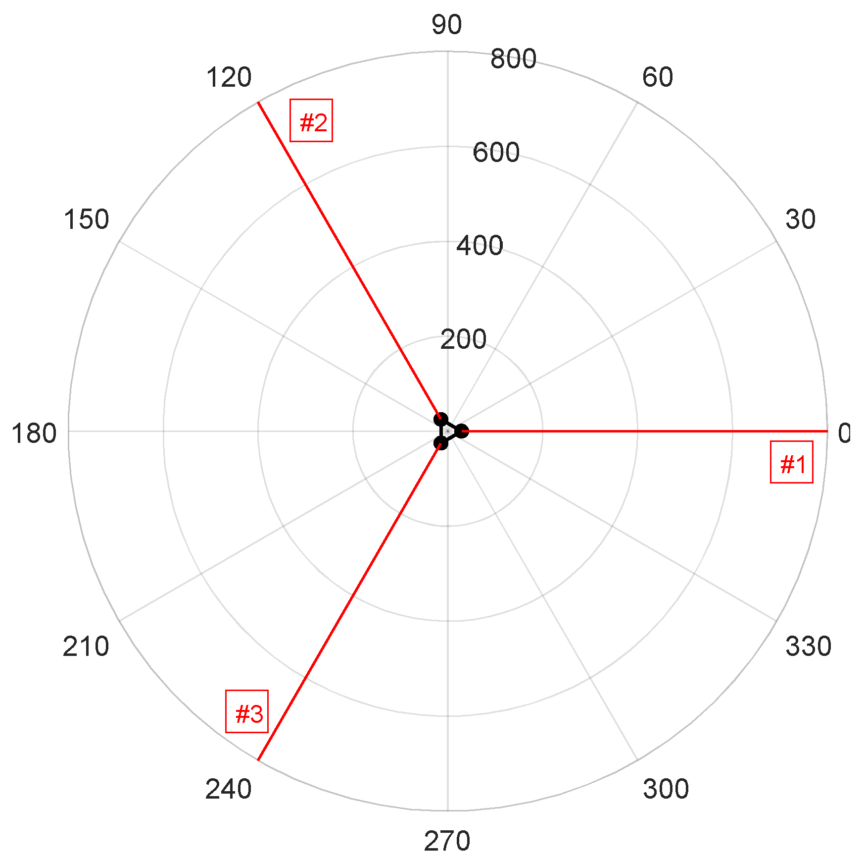
5.2. The Stationkeeping System

The FOWT is equipped with a three-line spread mooring system, consisting of stud-link chain cables. The main properties of the stationkeeping system and the soil conditions are listed in

Table 2. Main properties of the reference stationkeeping system.

Water Depth	200 m
Chain cable diameter	76.6 mm
Material grade	R3
Material Young modulus	81,764 MPa
Total line length/line length on the seabed at rest	835.5/165.4 m
Fairlead horizontal/vertical coordinate as regards the local reference system	796.6/186.0 m
Intercept parameter of the S–N curve	1.2 × 1011 MPa
Slope parameter of the S–N curve	3.0
Seabed drag coefficient	1.0

, while a sketch of the mooring layout is depicted in Figure 3.

5.3. Selection of Reference Conditions

The benchmark study, carried out in Section 6, was performed based on the reference environmental conditions recently investigated by Xu et al. [36] and listed in

Table 3. Main data of reference conditions.

Load Condition	${\mathit{H}}_{\mathit{s}}\left[\mathbf{m}\right]$	${\mathit{T}}_{\mathit{p}}\left[\mathbf{s}\right]$	${\mathit{v}}_{\mathit{w}}[\mathbf{m}/\mathbf{s}]$	Reference Scenario
LC1	1.96	9.72	4.0	Power production
LC2	2.53	9.85	8.0	Power production
LC3	3.20	10.11	12.0	Power production
LC4	3.97	10.44	16.0	Power production
LC5	4.80	10.82	20.0	Power production
LC6	5.69	11.23	24.0	Power production
LC7	7.64	12.08	32.0	Parked wind turbine
LC8	9.77	12.95	40.0	Parked wind turbine

. They are representative of both power production and parked wind turbine situations. The sea state condition is described by the JONSWAP spectrum [39], with a significant wave height, $H_s$, ranging from 1.96 to 9.77 m and a wave peak period ranging from 9.72 to 12.95 s. The wind climate was described by the 10 min wind speed at hub height, combined with the Norwegian Petroleum Directorate wind spectrum [36], which is representative of the turbulent component. Wave and wind loads were assumed to be codirectional, with heading angle equal to 0°, to exert the highest loads in the mooring line #1.

5.4. Preliminary Analysis

Before carrying out the benchmark study, a preliminary analysis was performed to test the effectiveness and robustness of the hydrodynamic model developed in MATLAB. Figure 4 and Figure 5 provide the mean values, $\mu ,$ and the standard deviations, $\sigma ,$ of the stress process in the mooring line #1, obtained by the numerical model, currently developed in MATLAB, and by the numerical simulations performed by Xu et al. [36] by the commercial code SIMA [55]. The SIMA software, currently licensed and supported by the Det Norske Veritas, is a complete tool for the simulation of marine operations from modelling to results, which include lifting of topsides and modules, offshore wind turbine installation, offshore crane operations, subsea installations, transportation and installation of TLPs and towing operations, among others. The software, widely tested and validated in the past, was recently extended to FOWTs, and it can be considered a reliable and effective mean of comparison. By the analysis of current results, it was gathered that the numerical code, developed in MATLAB allows the efficient estimation of the mean value and the standard deviation of the stress process, with errors less than 5%.

6. Benchmark Study

6.1. Assessment of the Stress Process in the Mooring Lines

The stress process in mooring line#1, corresponding to a typical 3 h storm duration, is plotted in Figure 6a–h, with a sampling frequency of 5 Hz. As can be gathered from the relevant stress histories, the standard deviation of the stress process increased along with the sea state severity. In this respect, the load conditions from LC1 to LC6, which refer to the power production mode, were clearly dominated by the low-frequency component of the stress process, while the low- and wave-frequency components of the stress process were comparable in the last two conditions, which refer to the parked wind turbine situation. These outcomes will be further investigated by the fatigue analysis, performed in Section 6.2 and Section 6.3, by the time-domain and spectral models, respectively.

6.2. Time-Domain Analysis of the Stress Process

Table 4. Fatigue assessment by time-domain analysis.

Load Condition	${\mathit{\sigma }}_{\mathit{j},\mathit{L}}$	${\mathit{\sigma }}_{\mathit{j},\mathit{W}}$	${\mathit{\sigma }}_{\mathit{j}}$	${\mathit{\nu }}_{\mathit{j},\mathit{L}}$	${\mathit{\nu }}_{\mathit{j},\mathit{W}}$	${\mathit{\nu }}_{\mathit{j}}$	$\overline{\mathit{d}}/{\mathit{T}}_{\mathit{j}}$
	[MPa]	[MPa]	[MPa]	[Hz]	[Hz]	[Hz]	[Hz]
LC1	1.399	0.719	1.573	0.0086	0.1029	0.0476	4.649 × 10−11
LC2	5.051	1.468	5.260		0.1015	0.0295	1.077 × 10−9
LC3	9.563	2.854	9.979		0.0989	0.0295	7.340 × 10−9
LC4	8.570	3.174	9.139		0.0958	0.0342	6.550 × 10−9
LC5	8.908	4.170	9.835		0.0924	0.0400	9.529 × 10−9
LC6	9.647	5.371	11.041		0.0890	0.0440	1.483 × 10−8
LC7	8.375	7.121	10.993		0.0828	0.0540	1.799 × 10−8
LC8	16.799	15.144	22.617		0.0772	0.0521	1.511 × 10−7

provides the fatigue assessment of mooring line #1 by time-domain analysis, considering a separation frequency equal to 0.05 Hz. The cumulative fatigue damage per unit time is reported for each load condition, together with the standard deviations and up-crossing rates of the low- and wave-frequency components of the stress process. In this respect, it must be pointed out that the up-crossing rate of the low-frequency component was constant according to the first of Equation (14), as it depends on the surge natural period of the FOWT, equal to 116 s. The effectiveness of this assumption is checked in Section 7.

6.3. Spectral Analysis of the Stress Process

The spectra of the stress process in mooring line #1, determined by Welch and Thomson methods, are plotted in Figure 7a–h using black continuous and red dashed lines, respectively. In all cases, the separation frequency was set equal to 0.05 Hz. In addition, the low- and wave-frequency components of the stress process were clearly detectable. The former is due to the combined action of the slowly varying drift forces and the turbulent component of the wind forces; the latter, instead, is related to the first-order wave forces. The cumulative fatigue damage per unit time and the relevant fatigue parameters required by the combined spectrum method are reported in

Table 5. Fatigue assessment by spectral analysis—Welch method.

Load Condition	${\mathit{\sigma }}_{\mathit{j},\mathit{L}}$	${\mathit{\sigma }}_{\mathit{j},\mathit{W}}$	${\mathit{\sigma }}_{\mathit{j}}$	${\mathit{\nu }}_{\mathit{j},\mathit{L}}$	${\mathit{\nu }}_{\mathit{j},\mathit{W}}$	${\mathit{\nu }}_{\mathit{j}}$	$\overline{\mathit{d}}/{\mathit{T}}_{\mathit{j}}$
	[MPa]	[MPa]	[MPa]	[Hz]	[Hz]	[Hz]	[Hz]
LC1	1.419	0.686	1.576	0.0078	0.1021	0.0450	4.415 × 10−11
LC2	5.055	1.465	5.263	0.0095	0.1016	0.0297	1.086 × 10−9
LC3	9.582	2.806	9.984	0.0126	0.1001	0.0306	7.643 × 10−9
LC4	8.570	3.201	9.148	0.0105	0.0956	0.0348	6.686 × 10−9
LC5	8.912	4.195	9.850	0.0109	0.0926	0.0407	9.742 × 10−9
LC6	9.719	5.283	11.062	0.0102	0.0900	0.0439	1.490 × 10−8
LC7	8.359	7.188	11.025	0.0090	0.0843	0.0554	1.860 × 10−8
LC8	17.095	14.883	22.666	0.0116	0.0816	0.0543	1.584 × 10−7

and

Table 6. Fatigue assessment by spectral analysis—Thomson method.

Load Condition	${\mathit{\sigma }}_{\mathit{j},\mathit{L}}$	${\mathit{\sigma }}_{\mathit{j},\mathit{W}}$	${\mathit{\sigma }}_{\mathit{j}}$	${\mathit{\nu }}_{\mathit{j},\mathit{L}}$	${\mathit{\nu }}_{\mathit{j},\mathit{W}}$	${\mathit{\nu }}_{\mathit{j}}$	$\overline{\mathit{d}}/{\mathit{T}}_{\mathit{j}}$
	[MPa]	[MPa]	[MPa]	[Hz]	[Hz]	[Hz]	[Hz]
LC1	1.457	0.603	1.576	0.0078	0.1023	0.0398	3.905 × 10−11
LC2	5.094	1.325	5.263	0.0094	0.1017	0.0272	9.930 × 10−10
LC3	9.643	2.588	9.985	0.0123	0.1002	0.0286	7.124 × 10−9
LC4	8.647	2.987	9.148	0.0103	0.0957	0.0327	6.282 × 10−9
LC5	9.025	3.947	9.850	0.0108	0.0927	0.0384	9.207 × 10−9
LC6	9.877	4.982	11.063	0.0102	0.0899	0.0415	1.408 × 10−8
LC7	8.488	7.035	11.025	0.0089	0.0843	0.0542	1.820 × 10−8
LC8	17.658	14.211	22.666	0.0121	0.0816	0.0520	1.518 × 10−7

. By a comparative analysis between the cumulative fatigue damage provided by the Welch and Thomson methods, the two spectral analysis techniques provide comparable results, in terms of standard deviations and up-crossing rates of both low- and wave-frequency components of the stress process in the mooring line #1. Further details are provided in Section 7.

7. Discussion

Figure 8a–d provides a comparative study between the time-domain analysis and the advanced spectral reconstruction models, focusing on the estimated values of the standard deviations and up-crossing rates of the low- and wave-frequency components. As concerns the stress process standard deviation, a very good agreement was reached in all cases. Some differences between time- and frequency-domain analysis arose with reference to the up-crossing rate of the low-frequency component of the stress process. Anyway, these differences had a negligible impact on the cumulative fatigue damage per unit time reported in Figure 9. In fact, a substantial agreement was in all cases recognized between time-domain and spectral models, with absolute errors generally less than 5%. This outcome was partly due to the endorsement of the combined spectrum approach in both cases, but it also highlighted that both simplified time-domain and advanced spectral analysis can be applied to assess the cumulative fatigue damage in the mooring lines, with almost the same level of accuracy.

Based on current results, some main outcomes can be stressed:

(i)

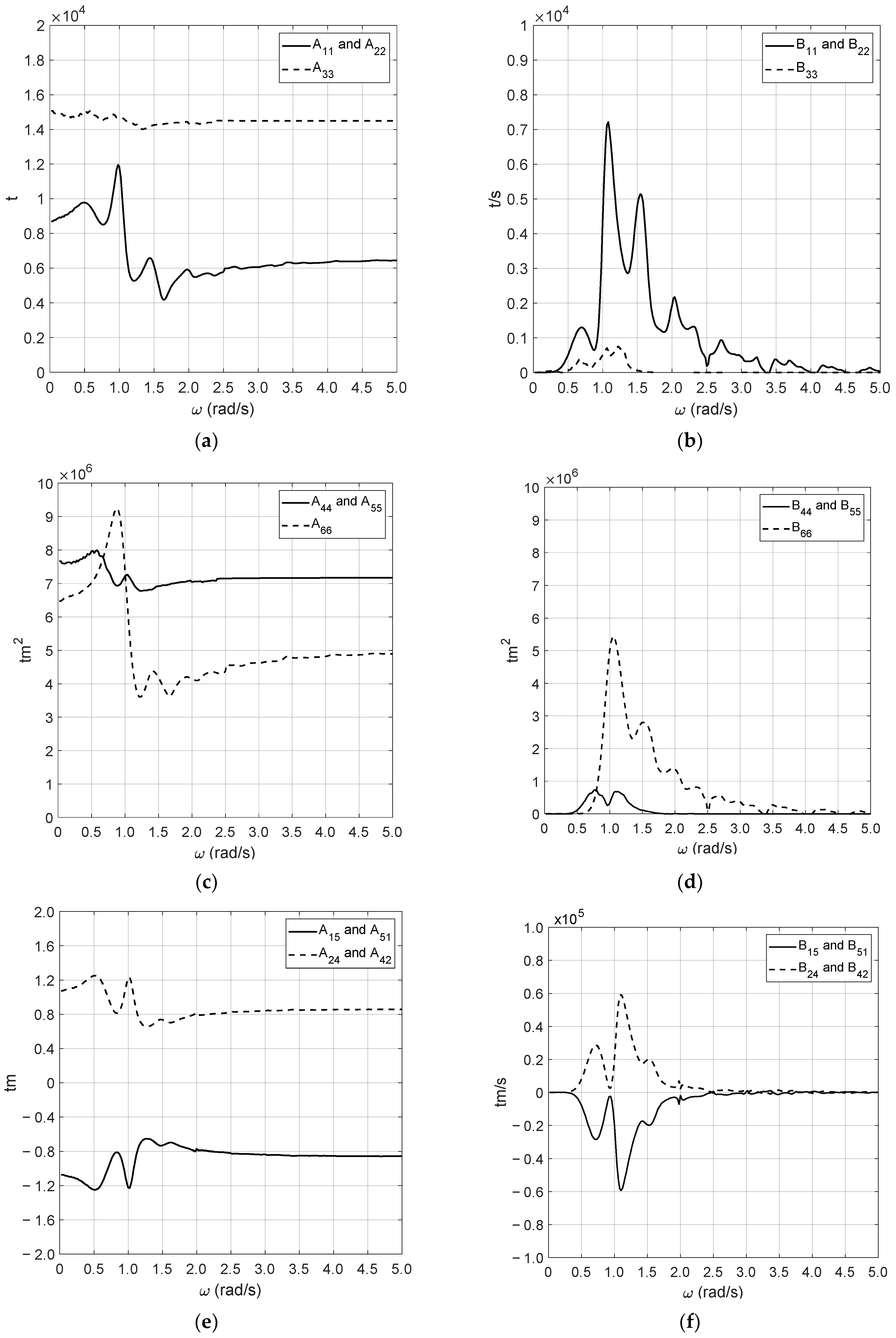
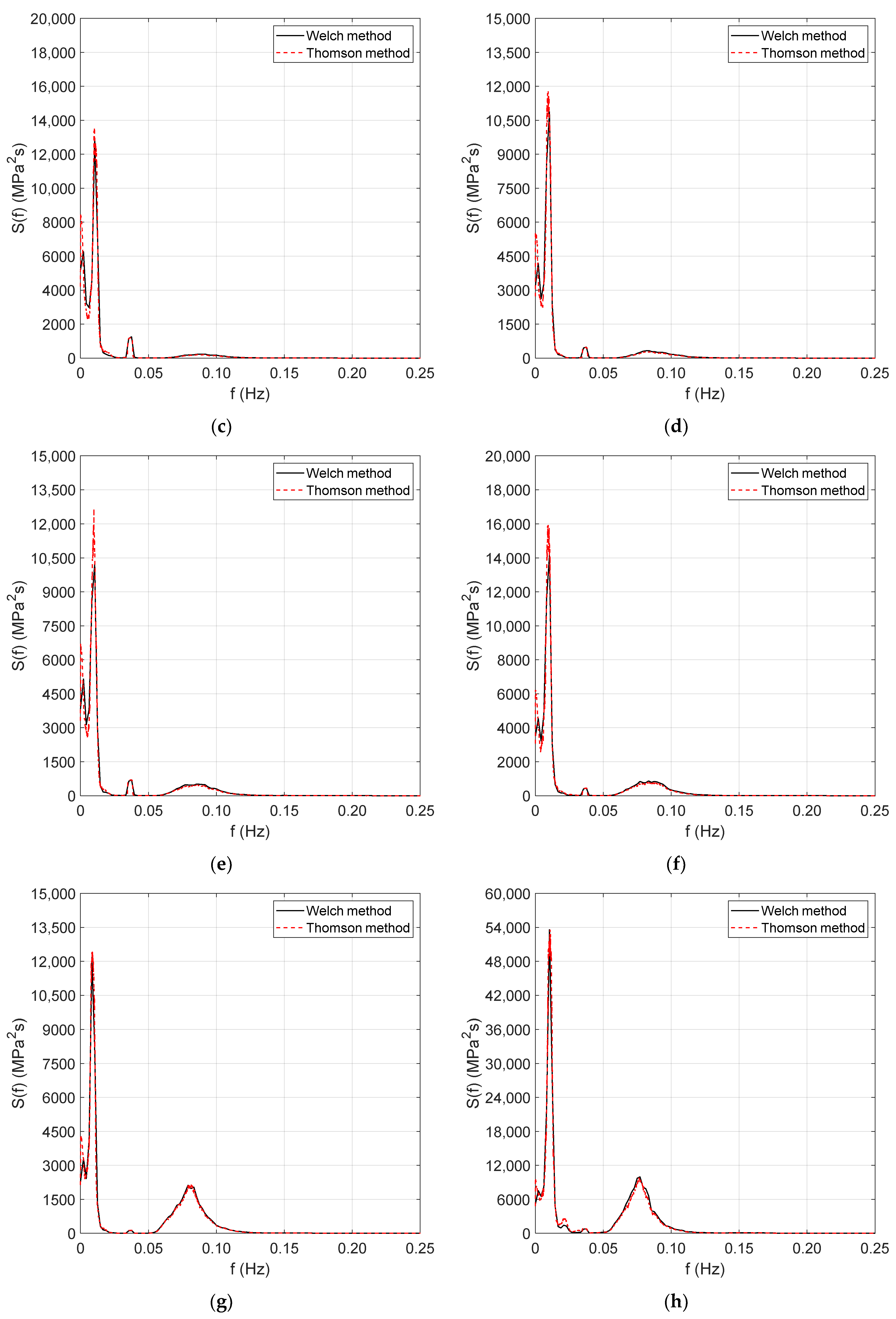
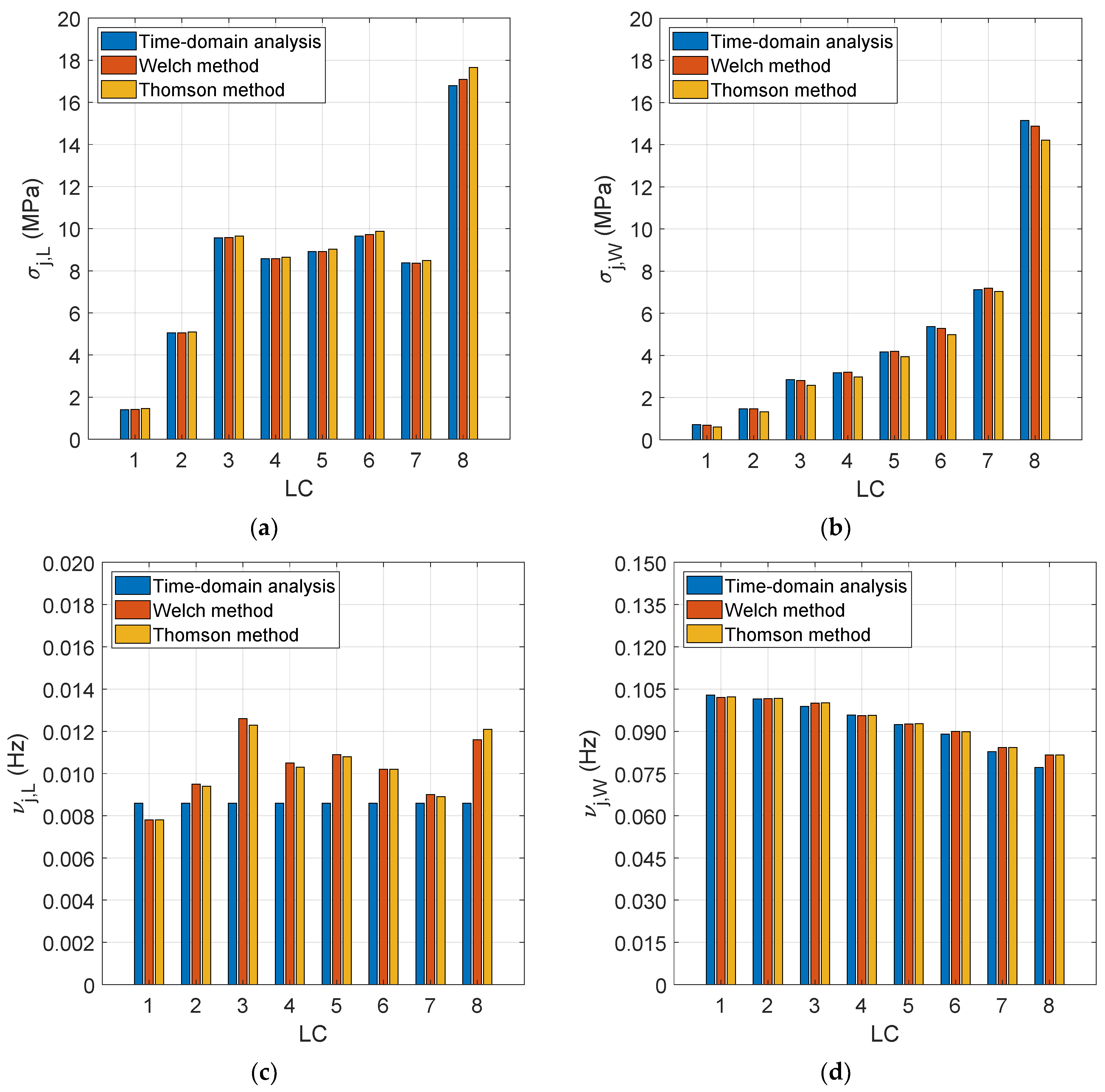
Time-domain models are accurate enough, at least when a variety of cases need to be analysed to assess the design fatigue life of the mooring lines. In this respect, the up-crossing rate of the low- and wave-frequency components of the stress process can be assumed to be equal to the surge/sway natural period of the tri-floater platform and the wave peak period of the relevant sea state condition. These assumptions are accurate enough, as can be gathered from Figure 8c,d.

(ii)

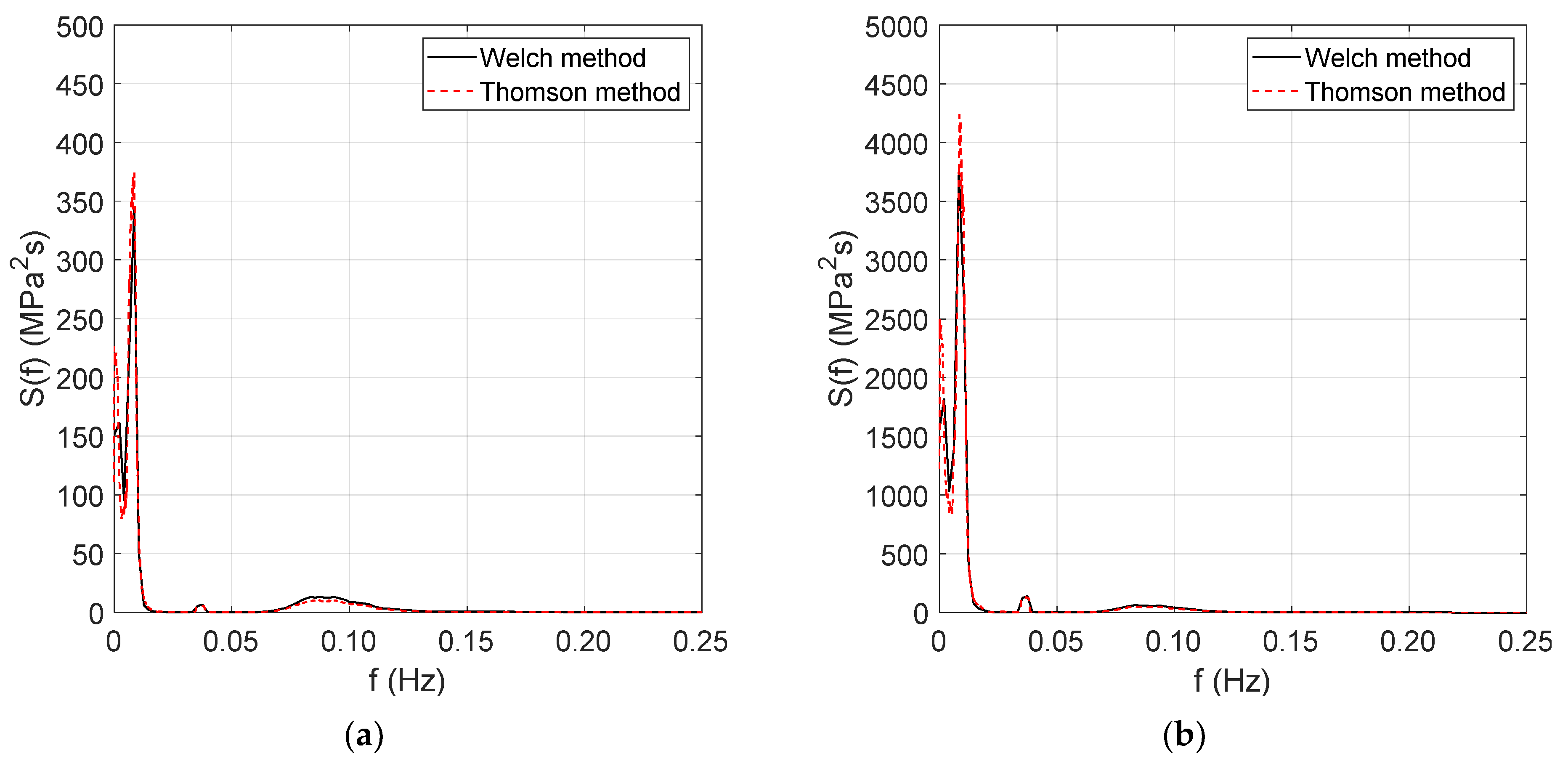
Welch and Thomson methods allow accurate detection of the low- and wave-frequency components of the stress process once the partitioning frequency is provided. It was verified that the separation frequency of 0.05 Hz allowed accurate detection of the low- and wave-frequency components.

(iii)

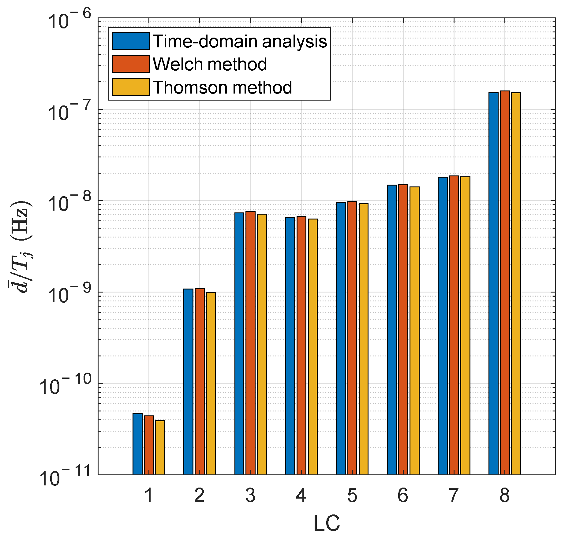
It is quite challenging to identify which spectral analysis method, between the Welch and Thomson models, is the most suitable one. Presumably both methods can be applied with the same confidence, at least based on current results, provided they lead to almost the same cumulative fatigue damage per unit time in all the analysed loading conditions.

8. Conclusions

The paper focused on the assessment of the cumulative fatigue damage in the mooring lines of an FOWT, deployed on intermediate water depth, by time-domain and advanced spectral analysis methods. After a brief review about the state-of-art, the nonlinear time-domain hydrodynamic model, was provided and the various force components were separately discussed. The cumulative fatigue damage in the mooring line #1 was assessed by the combined spectrum approach, accounting for both low- and wave-frequency components of the stress process, as typically occurs for offshore structures. The fatigue analysis was carried out by time-domain analysis and advanced spectral reconstruction models, based on Welch and Thomson methods.

In order to test the effectiveness of both time- and frequency-domain models, a benchmark study was performed, assuming as the reference FOWT the OC4-DeepCwind tri-floater platform, equipped with the NREL 5 MW wind turbine. Several loading conditions, representative of both power production and parked wind turbine situations, were considered to investigate the incidence of met-ocean conditions on the assessment of the fatigue cumulative damage. As stressed in Section 8, a very good agreement between time- and frequency-domain models, was in all cases recognized, confirming that the former is accurate enough when a variety of cases need to be analysed, while the latter provides a more rational approach for the assessment of the main fatigue parameters. In this respect, the Welch and Thomson methods were revealed to be very promising techniques for the reliable assessment of the mooring fatigue life, as they allow the proper estimation of all the fatigue parameters, required by the combined stress method. The current results are encouraging for future research, devoted to endorsing spectral analysis in the assessment of the mooring line fatigue life, in view of a more reliable and rational design approach of stationkeeping systems, and eventually to update the mooring-related safety factors, embodied in current rules and guidelines.

References

1. Xue, X.; Chen, N.Z.; Wu, Y.; Xiong, Y.; Guo, Y. Mooring system fatigue analysis for a semi-submersible. Ocean. Eng. 2018, 156, 550–563. [Google Scholar] [CrossRef]
2. European Union Commission. Horizon 2020 Work Programme 2018–2020 “Secure, Clean and Efficient Energy”; The European Commission: Bruxelles, Belgium, 2018. [Google Scholar]
3. Kvitrud, A. Lessons learned from Norwegian mooring line failures 2010–2013. In Proceedings of the ASME 33rd International Conference on Ocean, Offshore and Arctic Engineering, San Francisco, CA, USA, 8–13 June 2014. [Google Scholar]
4. de Laval, G. Fatigue tests on anchor chain cable. In Proceedings of the Offshore Technology Conference, Houston, TX, USA, 18–20 April 1971. [Google Scholar]
5. van Helvoirt, L.C. Static and fatigue tests on chain links and chain connecting links. In Proceedings of the Offshore Technology Conference, Houston, TX, USA, 3–6 May 1982. [Google Scholar]
6. Horde, G.O.; Moan, T. Fatigue and overload reliability of mooring systems. In Proceedings of the 7th International Offshore and Polar Engineering Conference, Honolulu, HI, USA, 25–30 May 1997. [Google Scholar]
7. Gao, Z.; Moan, T. Fatigue damage induced by nonGaussian bimodal wave loading in mooring lines. Appl. Ocean. Res. 2007, 29, 45–54. [Google Scholar] [CrossRef]
8. Xu, T.J.; Zhao, Y.P.; Dong, G.H.; Bi, C.W. Fatigue analysis of mooring system for net cage under random loads. Aquac. Eng. 2014, 58, 59–68. [Google Scholar] [CrossRef]
9. Brommundt, M.; Krause, L.; Merz, K.; Muskulus, M. Mooring system optimization for floating wind turbines using frequency domain analysis. Energy Procedia 2012, 24, 289–296. [Google Scholar] [CrossRef] [Green Version]
10. Benassai, G.; Campanile, A.; Piscopo, V.; Scamardella, A. Mooring control of semi-submersible structures for wind turbines. Procedia Eng. 2014, 70, 132–141. [Google Scholar] [CrossRef]
11. Benassai, G.; Campanile, A.; Piscopo, V.; Scamardella, A. Ultimate and accidental limit state design for mooring systems of floating offshore wind turbines. Ocean. Eng. 2014, 92, 64–74. [Google Scholar] [CrossRef]
12. Kim, H.; Choung, J.; Jeon, G. Design of mooring lines of floating offshore wind turbine in Jeju offshore area. In Proceedings of the 33rd International Conference on Ocean, Offshore and Arctic Engineering, San Francisco, CA, USA, 8–13 June 2014. [Google Scholar]
13. Hall, M.; Goupee, A. Validation of a lumped-mass mooring line model with DeepCwind semisubmersible model test data. Ocean. Eng. 2015, 104, 590–603. [Google Scholar] [CrossRef] [Green Version]
14. Campanile, A.; Piscopo, V.; Scamardella, A. Mooring design and selection for floating offshore wind turbines on intermediate and deep-water depths. Ocean. Eng. 2018, 148, 349–360. [Google Scholar] [CrossRef]
15. DnV-GL. Position Mooring. Offshore Standard DNVGL-OS-E301. 2018. Available online: https://rules.dnv.com/docs/pdf/DNV/os/2018-07/dnvgl-os-e301.pdf (accessed on 19 October 2021).
16. Winterstein, S.R. Nonlinear vibration models for extremes and fatigue. J. Eng. Mech. 1988, 114, 1772–1790. [Google Scholar] [CrossRef]
17. Jiao, G.; Moan, T. Probabilistic analysis of fatigue due to Gaussian load processes. Probabilistic Eng. Mech. 1990, 5, 76–83. [Google Scholar] [CrossRef]
18. Fu, T.T.; Cebon, D. Predicting fatigue lives for bi-modal stress spectral densities. Int. J. Fatigue 2000, 22, 11–21. [Google Scholar] [CrossRef]
19. Low, Y.M. A method for accurate estimation of the fatigue damage induced by bimodal processes. Probabilistic Eng. Mech. 2010, 25, 75–85. [Google Scholar] [CrossRef]
20. Gao, Z.; Zheng, X.Y. An improved spectral discretization method for fatigue damage assessment of bimodal Gaussian processes. Int. J. Fatigue 2019, 119, 268–280. [Google Scholar] [CrossRef]
21. Jun, S.-H.; Park, J.-B. Development of a novel fatigue damage model for Gaussian wide band stress responses using numerical approximation methods. Int. J. Nav. Archit. Ocean. Eng. 2020, 12, 755–767. [Google Scholar] [CrossRef]
22. Ma, Y.; Han, C.; Qu, X. Fatigue assessment method of marine structures subjected to two Gaussian random loads. Ocean. Eng. 2021, 165, 107–122. [Google Scholar] [CrossRef]
23. Wolfsteiner, P.; Trapp, A. Fatigue life due to non-Gaussian excitation—An analysis of the Fatigue Damage Spectrum using Higher Order Spectra. Int. J. Fatigue 2019, 127, 203–216. [Google Scholar] [CrossRef]
24. Kim, H.-J.; Jang, B.-S.; Kim, J.D. Fatigue-damage prediction for ship and offshore structures under widebanded non-Gaussian random loadings Part I: Approximation of cycle distribution in wide-banded gaussian random processes. Appl. Ocean. Res. 2020, 101, 102294. [Google Scholar] [CrossRef]
25. Marques, J.M.E.; Benasciutti, D. More on variance of fatigue damage in non-Gaussian random loadings—Effect of skewness and kurtosis. Procedia Struct. Integr. 2020, 25, 101–111. [Google Scholar] [CrossRef]
26. Gao, S.; Zheng, X.Y.; Wang, B.; Zhao, S.; Li, W. Assessment of fatigue damage induced by Non-Gaussian bimodal processes with emphasis on spectral methods. Ocean. Eng. 2021, 220, 108489. [Google Scholar] [CrossRef]
27. Kim, H.-J.; Jang, B.-S. Fatigue life prediction of ship and offshore structures under wide-banded non-Gaussian random loadings Part II: Extension to wide-banded non-Gaussian random processes. Appl. Ocean. Res. 2021, 106, 102480. [Google Scholar] [CrossRef]
28. Marques, J.M.E.; Benasciutti, D. Variance of the fatigue damage in non-Gaussian stochastic processes with narrow-band power spectrum. Struct. Saf. 2021, 93, 102131. [Google Scholar] [CrossRef]
29. Robertson, A.; Jonkman, J.M.; Masciola, M.; Song, H.; Goupee, A.; Coulling, A.; Luan, C. Definition of the Semisubmersible Floating System for Phase II of OC4; Technical Report NREL/TP-5000-60601; National Renewable Energy Laboratory: Golden, CO, USA, 2014.
30. Jonkman, J.M. Dynamics Modelling and Loads Analysis of an Offshore Floating Wind Turbine; Technical Report NREL/TP-5000-41958; National Renewable Energy Laboratory: Golden, CO, USA, 2007.
31. Zhao, Z.; Wang, W.; Shi, W.; Ki, X. Effects of second-order hydrodynamics on an ultra-large semi-submersible floating offshore wind turbine. Structures 2020, 28, 2260–2275. [Google Scholar] [CrossRef]
32. Barrera, C.; Battistella, T.; Guanche, R.; Lozada, I.J. Mooring system fatigue analysis of a floating offshore wind turbine. Ocean. Eng. 2020, 195, 106670. [Google Scholar] [CrossRef]
33. Zhang, L.; Shi, W.; Karimirad, M.; Michailides, C.; Jiang, Z. Second-order hydrodynamic effects on the response of three semisubmersible floating offshore wind turbines. Ocean. Eng. 2020, 207, 107371. [Google Scholar] [CrossRef]
34. Cummins, W.E. The impulse response function and ship motions. Schiffstechnik 1962, 9, 101–109. [Google Scholar]
35. Newman, J.N. Second-order, slowly varying forces on vessels in irregular waves. In Proceedings of the International Symposium on Dynamics of Marine Vehicles and Structures in Waves, University College London, London, UK, 1–5 April 1974; pp. 182–186. [Google Scholar]
36. Xu, K.; Larsen, K.; Shao, Y.; Zhang, M.; Gao, Z.; Moan, T. Design and comparative analysis of alternating mooring systems for floating wind turbines in shallow water with emphasis on ultimate limit state design. Ocean. Eng. 2021, 219, 108377. [Google Scholar] [CrossRef]
37. Wan, L.; Ghao, Z.; Moan, T.; Lugni, C. Comparative experimental study of the survivability of a combined wind and wave energy converter in two testing facilities. Ocean. Eng. 2016, 111, 82–94. [Google Scholar] [CrossRef] [Green Version]
38. Hansen, M.O.L. Aerodynamics of Wind Turbines; Routledge: Abingdon-on-Thames, UK, 2015. [Google Scholar]
39. DnV. Environmental Conditions and Environmental Loads. Recommended Practice DNV-RP-C205, 2014. Available online: https://rules.dnv.com/docs/pdf/dnvpm/codes/docs/2014-04/RP-C205.pdf (accessed on 19 October 2021).
40. Jonkman, J.M. Dynamics of Offshore Floating Wind Turbines—Model Development and Verification. Wind. Energy 2009, 12, 459–492. [Google Scholar] [CrossRef]
41. Trubat, P.; Molins, C.; Gironella, X. Wave hydrodynamic forces over mooring lines on floating offshore wind turbines. Ocean. Eng. 2020, 195, 106730. [Google Scholar] [CrossRef]
42. Ma, Y.; Hu, Z.; Xiao, L. Wind-wave induced dynamic response analysis for motions and mooring loads of a spar-type offshore floating wind turbine. J. Hydrodyn. 2014, 26, 865–874. [Google Scholar] [CrossRef]
43. MathWorks. Matlab User Guide R2020b, 2020. Available online: https://it.mathworks.com/help/matlab/ (accessed on 19 October 2021).
44. Saf onov, M.G.; Chiang, R.Y. A Schur Method for Balanced Model Reduction. IEEE Trans. Autom. Control. 1989, 34, 729–733. [Google Scholar] [CrossRef]
45. Kung, S.Y. A New Identification and Model Reduction Algorithm via Singular Value Decompositions. In Proceedings of the 12th Asilomar Conference on Circuits, Systems and Computers (Institute of Electrical and Electronic Engineers), New York, NY, USA, 6–8 November 1978; pp. 705–714. [Google Scholar]
46. Babarit, A.; Delhommeau, G. Theoretical and numerical aspects of the open-source BEM solver NEMOH. In Proceedings of the 11th European Wave and Tidal Energy Conference, Nantes, France, 6–11 September 2015; pp. 1–12. [Google Scholar]
47. Miner, M.A. Cumulative damage in fatigue. J. Appl. Mech. 1945, 12, 159–164. [Google Scholar] [CrossRef]
48. Xu, S.; Guedes Soares, C. Evaluation of spectral methods for long term fatigue damage analysis of synthetic fibre mooring ropes based on experimental data. Ocean. Eng. 2021, 226, 108842. [Google Scholar] [CrossRef]
49. DnV-GL. Standard DNVGL-ST-0437; Loads and Site Conditions for Wind Turbines. Det Norske Veritas Group: Høvik, Norway, 2016.
50. Percival, D.B.; Walden, A.T. Spectral Analysis for Physical Applications; Cambridge University Press: Cambridge, UK, 1993. [Google Scholar]
51. Welch, P.D. The Use of Fast Fourier Transform for the Estimation of Power Spectra: A Method Based on Time Averaging over Short Modified Periodograms. IEEE Trans. Audio Electroacoust. 1967, 15, 70–73. [Google Scholar] [CrossRef] [Green Version]
52. Thomson, D.J. Spectrum Estimation and Harmonic Analysis. Proc. IEEE 1982, 70, 1055–1096. [Google Scholar] [CrossRef] [Green Version]
53. Marple, S.L. Digital Spectral Analysis; Prentice—Hall: Englewood Cliffs, NJ, USA, 1987. [Google Scholar]
54. Piscopo, V.; Scamardella, A. Comparative study among non-redundant and redundant stationkeeping systems for Floating Offshore Wind Turbines on intermediate water depth. Ocean. Eng. 2021, 241, 110047. [Google Scholar] [CrossRef]
55. SINTEF Ocean. SIMO 4.14.0 User Guide, 2018. Available online: https://projects.dnvgl.com/sesam/status/Simo/SIMO-release-notes_4.14.0.pdf (accessed on 19 October 2021).
56. Braccesi, C.; Cianetti, F.; Lori, G.; Pioli, D. The frequency domain approach in virtual fatigue estimation of non-linear systems: The problem of non-Gaussian states of stress. Int. J. Fatigue 2009, 31, 766–775. [Google Scholar] [CrossRef]
57. Chuang, Z.; Liu, S.; Lu, Y. Influence of second order wave excitation loads on coupled response of an offshore floating wind turbine. Int. J. Nav. Archit. Ocean. Eng. 2020, 12, 367–375. [Google Scholar] [CrossRef]
Figure 1. Reference layout of the OC4-DeepCwind platform (the symbol # means line number).
Jmse 10 00037 g001
Figure 2. Thrust curve of the NREL 5 MW wind turbine.
Jmse 10 00037 g002
Figure 3. Layout of the reference stationkeeping system (the symbol # means line number).
Jmse 10 00037 g003
Figure 4. Comparative analysis—mean value of stress history in line #1.
Jmse 10 00037 g004
Figure 5. Comparative analysis—standard deviation of stress history in line #1.
Jmse 10 00037 g005
Figure 6. Stress history in line #1. (a) Load condition LC1; (b) load condition LC2; (c) load condition LC3; (d) load condition LC4; (e) load condition LC5; (f) load condition LC6; (g) load condition LC7; (h) load condition LC8.
Jmse 10 00037 g006aJmse 10 00037 g006b
Figure 7. Spectra of the stress history in line #1. (a) Load condition LC1; (b) load condition LC2; (c) load condition LC3; (d) load condition LC4; (e) load condition LC5; (f) load condition LC6; (g) load condition LC7; (h) load condition LC8.
Jmse 10 00037 g007aJmse 10 00037 g007b
Figure 8. Comparative analysis between time- and frequency-domain models. (a) Standard deviation of the low-frequency stress component; (b) standard deviation of the wave-frequency stress component; (c) up-crossing rate of the low-frequency stress component; (d) up-crossing rate of the wave-frequency stress component.
Jmse 10 00037 g008
Figure 9. Assessment of cumulative fatigue damage per unit time.
Jmse 10 00037 g009