Study on the Motion Stability of the Autonomous Underwater Helicopter

Abstract

The hydrodynamic performance of a novel hovering autonomous underwater vehicle, the autonomous underwater helicopter (AUH), with an original disk-shaped hull (HG1) and an improved fore–aft asymmetric hull (HG3), is investigated by means of computational fluid dynamics with the adoption of overlapping mesh method. The hydrodynamic performance of the two hull shapes in surge motion with variation of the angle of attack is compared. The results show that HG3 has less resistance and higher motion stability compared to HG1. With the angle of attack reaching 10 degrees, both HG1 and HG3 achieve the maximum lift-to-drag ratio, which is higher for HG3 compared to HG1. Furthermore, based on the numerical simulation of the plane motion mechanism test (PMM) and according to Routh’s stability criterion, the horizontal movement and vertical movement stability indexes of HG1 and HG3 (${\mathrm{G}}_{\mathrm{H}}^{\mathrm{HG}1}=1.0$, ${\mathrm{G}}_{\mathrm{V}}^{\mathrm{HG}1}=49.7$, ${\mathrm{G}}_{\mathrm{H}}^{\mathrm{HG}2}=1.0$,${\mathrm{G}}_{\mathrm{V}}^{\mathrm{HG}3}=2.1$) are obtained, which further show that the AUH has better vertical movement stability than the torpedo-shaped AUV. Furthermore, the scale model tail velocity experiment indirectly shows that HG3 has better hydrodynamic performance than HG1.

1. Introduction

The seabed observation network is a platform to realize all-weather, in situ, long-term, continuous, real-time, and high-resolution observation from the seabed to the sea surface, which plays an important role in supporting the development of marine science [1,2]. As a supplement, mobile observation equipment, such as autonomous underwater vehicles (AUVs) and autonomous underwater gliders (AUGs), can quickly respond to emergencies in the target sea area and intensive observation [3], which can improve stereoscopic observation in the ocean, as shown in Figure 1.

AUVs have the ability to realizing long-distance and large-scale inspection. In the US, the Bluefin series AUV, jointly developed by the US naval graduate school and tuna robotics company, is a relatively mature AUV system platform that has been equipped by the US Navy [4]. Kongsberg Maritime, together with the Norwegian Defense Research Establishment (FFI), developed the HUGIN class AUV, which is used for seabed surveying and mapping in the deep sea [5,6]. In addition to large AUVs, some researchers have focused on developing small AUVs for inspection and mapping purposes. Complementary to the application fields of HUGIN, REMUS (designed by the Woods Hole Oceanographic Institute) is a very small and lightweight vehicle specially designed for coastal oceanography, the cost of which is much lower than that of HUGIN [7]. In Europe, the EU sponsored the project of the MARIUS AUV [8], which is one of the first non-torpedo-shaped submersibles. As for what it concerns, the traditional AUV has limited maneuverability due to its large fore–aft length scale compared to the other two directions, giving rise to a large turn-around radius [9]. On the other hand, AUGs such as the Seaglider AUG [10], the Spray AUG [11], etc., are types of AUVs that have been successfully applied in oceanographic sensing and data collection [12], equipped with temperature salt depth (CTD) and other sensors. AUGs can glide underwater by controlling their buoyancy and converting the lift on the wings into propulsive force without a power propulsion system [13], which, however, limits their operation under complex seabed conditions. Therefore, the deployment of AUVs and AUGs near the seabed with complex topography for close-up inspection encounters great difficulty.

A nearly disk-shaped autonomous underwater helicopter (AUH) capable of taking the movement in both horizontal (surge) or vertical (heave) directions was recently developed [14], realized by four horizontally arranged propellers and two vertically arranged propellers, as shown in Figure 2. Through the combination of horizontal motion and vertical motion, the AUH can realize long-range cruise, zero-diameter turning, and accurate landing and take-off on the seabed. Therefore, compared to the torpedo-shaped AUV and AUG, the AUH can also work as an ROV. As a result, adoption of the AUH can further promote underwater observation in the ocean combined with the underwater observation network, as shown in Figure 1. The basic parameters of the AUH of the current form (with the hull shape of HG1) are listed in

Table 1. Basic parameters of the current AUH (the HG1 geometry).

Parameter	Diameter $(\mathbf{mm}$)	Hight $\left(\mathbf{mm}\right)$	Weight $\left(\mathbf{kg}\right)$	Cruise Speed $(\mathbf{m}/\mathbf{s})$
Value	1557	801	$\le$300	$\le$2

. HG1 is improved through local modification at the rear part of the original hull geometry, which results in a fore–aft asymmetric structure (HG3), as shown in Figure 2d.

Numerical simulation using computational fluid dynamics (CFD) software is widely used in research on the hydrodynamic characteristics of AUVs [14,15,16,17,18,19,20,21], such as the effects of free-stream turbulence, hydrodynamic force coefficients, hydrodynamic characteristics of AUV over seabed [22,23,24], etc. For the AUH, Chen et al. applied both CFD results and the Routh stability criterion to identify the AUH motion stability [25]. The hydrodynamic interaction of an approaching ship with the wave effect [26], the water entry impact force [27], and the Magnus effect [25] are also studied by CFD methods. An et al. [28] proposed a parametric representation of the AUH’s profile and combined the surrogate model with a genetic algorithm to optimize the AUH’s profile, effectively improving its lift–drag ratio. Lin et al. [29] investigated the hydrodynamic performance of the disk-shaped AUH considering the asymmetry and instability of the flow field, as well as the effect of propellers at both surge and heave motions. However, at the present stage, research is still lacking on the location optimization of the hull shape to improve the hydrodynamic property of the AUH.

In this paper, the spatial motion equation of the AUH is derived, and the hydrodynamic coefficients of translation and rotation of the AUH with HG1 and HG3, respectively, are calculated numerically based on the overlapping mesh technology and the RNG $k-\epsilon$ turbulence model. The hydrodynamic stability of HG1 and HG3 with a change in the angle of attack (AOA) is analyzed. Finally, according to Routh’s stability criterion [30], the stability of the two shapes of the AUH in the horizontal and vertical planes is determined.

2. Mathematical Model of Motion Stability

2.1. Dynamic Equation

Motion control equations, including the kinematic equation and the dynamic equation, can completely describe the motion of a submersible and provide a mathematical basis for realizing motion control [31].

The kinematic equation refers to the coordinate transformation relationship between the expressions of submersible motion parameters in different coordinate systems. As shown in Figure 3, two common coordinate systems, the spatial fixed coordinate system $O_0{x}_0{y}_0{z}_0$ and the motion coordinate system $Oxyz$, are used to analyze the AUV motion process. Origin $O_0$ takes any point in space, origin $O$ is selected on the center of gravity of the submersible, the $Ox$ axis is along the bow direction, and the $Oz$ axis points to the bottom of the submersible. The position and attitude of the submersible can be expressed as

$${\mathit{\eta }}^{O_0}={\left[x_O, y_O, z_O, \varphi , \theta , \psi \right]}^{\mathrm{T}}$$

(1)

The velocity vector of the submersible is expressed as

$${\dot{\mathit{\eta }}}^{O_0}={\left[{\dot{x}}_O, {\dot{y}}_O, {\dot{z}}_O, \dot{\varphi }, \dot{\theta }, \dot{\psi }\right]}^{\mathrm{T}}$$

(2)

$${\mathit{V}}^O={\left[u, v, w, p, q, r\right]}^{\mathrm{T}}$$

(3)

where $\varphi , \theta , \psi$ represent roll angle, pitch angle, and yaw angle, respectively. $u, v, w$ represent the translational velocity in the three directions of $x, y, z$, and $p, q, r$ represents the rotational velocity in the three directions of $x, y, z$.

The dynamic equation of any underwater vehicle can be derived from the momentum theorem and momentum moment theorem. For translational and rotational motion, the following vector relations exist, respectively.

$$\mathrm{m}\frac{d{\mathit{V}}_G}{dt}=\mathit{F}, \frac{\mathrm{d}{\mathit{L}}_G}{dt}={\mathit{M}}_G$$

(4)

$${\mathit{V}}_G={\left[\begin{array}{ccc}u+q{z}_G-r{y}_G& v+r{x}_G-p{z}_G& w+p{y}_G-q{x}_G\end{array}\right]}^{\mathrm{T}}$$

(5)

$${\mathit{L}}_G={\left[\begin{array}{ccc}{I}_{xx}^{G}p-I_{xy}^{G}q-I_{xz}^{G}r& I_{yy}^{G}q-I_{yx}^{G}p-I_{yz}^{G}r& I_{zz}^{G}r-I_{zx}^{G}p-I_{zy}^{G}q\end{array}\right]}^{\mathrm{T}}$$

(6)

where $x_G, y_G, z_G$ represent the vector position of the center of gravity of the vehicle in the dynamic system, $I_{xx}^G,$ $I_{yy}^G, I_{zz}^G$ represent the moment of inertia of three axes, and $I_{xy}^G, I_{yz}^G, I_{zx}^G$ represent the inertia product of the moving system.

Therefore, the equation can be expressed as follows

$$\begin{gathered} \{\begin{array}{c}X=m\left[\left(\dot{u}-vr+wq\right)-x_G\left(q^2+r^2\right)+y_G\left(pq-\dot{r}\right)+z_G\left(pr+\dot{q}\right)\right]\\ Y=m\left[\left(\dot{v}-wp+ur\right)-y_G\left(r^2+p^2\right)+z_G\left(qr-\dot{p}\right)+x_G\left(qp+\dot{r}\right)\right]\\ Z=m\left[\left(\dot{w}-uq+vp\right)-z_G\left(p^2+q^2\right)+x_G\left(rp-\dot{q}\right)+y_G\left(rp+\dot{p}\right)\right]\\ K=I_{xx}\dot{p}+\left(I_{zz}-I_{yy}\right)qr-\left(\dot{r}+pq\right)I_{xz}+\left(r^2-q^2\right)I_{yz}+\left(pr-\dot{q}\right)I_{xy}+ \\ m\left[y_G\left(\dot{w}-uq+vp\right)-z_G\left(\dot{v}-wp+ur\right)\right]\\ M=I_{yy}\dot{q}+\left(I_{xx}-I_{zz}\right)rp-\left(\dot{p}+qr\right)I_{xy}+\left(p^2-r^2\right)I_{zx}+\left(qp-\dot{r}\right)I_{yz}+ \\ m\left[z_G\left(\dot{u}-vr+wq\right)-x_G\left(\dot{w}-uq+vp\right)\right]\\ N=I_{zz}\dot{r}+\left(I_{yy}-I_{xx}\right)pq-\left(\dot{q}+rp\right)I_{yz}+\left(q^2-P^2\right)I_{xy}+\left(rq-\dot{p}\right)I_{zx}+ \\ m\left[x_G\left(\dot{v}-wp+ur\right)-y_G\left(\dot{u}-vr+wq\right)\right]\end{array} \end{gathered}$$

(7)

Since the origin of the dynamic system coincides with the center of gravity of the AUH and the coordinate axis coincides with the three principal inertial axes, $x_G, y_G, z_G$ is zero, and $I_{xy}=I_{yz}=I_{yx}=I_{zy}=I_{zx}=I_{xz}=0$. Therefore, the equation is simplified as

$$\{\begin{array}{c}X=m\left(\dot{u}-vr+wq\right)\\ Y=m\left(\dot{v}-wp+ur\right)\\ Z=m(\dot{w-uq+vp)}\\ K=I_{xx}\dot{p}+\left(I_{zz}-I_{yy}\right)qr\\ M=I_{yy}\dot{q}+\left(I_{xx}+I_{zz}\right)rp\\ N=I_{zz}\dot{r}+\left(I_{yy}-I_{xx}\right)pq\end{array}$$

(8)

However, when solving the problem of the motion control of a submersible, it is most important to obtain the information of the external force and moment ${\mathit{\tau }}_{RB}$ acting on it. In Equation (9), $\mathit{g}\left(\mathit{\eta }\right)$ represents static forces and moments, ${\mathit{\tau }}_H$ represents hydrodynamic forces and moments, ${\mathit{\tau }}_E$ represents environmental forces and moments, and $\mathit{\tau }$ represents the propulsion control force and moments.

$${\mathit{\tau }}_{RB}=-\mathit{g}\left(\mathit{\eta }\right)+{\mathit{\tau }}_H+{\mathit{\tau }}_E+\mathit{\tau }$$

(9)

Suppose the gravity and buoyancy of the AUH are $W$ and $B$, respectively. According to the pitch angle $\theta$ and the heel angle $\varphi$, the static force and moment can be obtained as the following equation

$$\mathit{g}\left(\mathit{\eta }\right)=-\left[\begin{array}{c}-\left(W-B\right)sin\theta \\ \left(W-B\right)cos\theta sin\varphi \\ \left(W-B\right)cos\theta sin\varphi \\ \left(y_{G}W-y_{B}B\right)cos\theta cos\varphi -\left(z_{G}W-z_{B}B\right)cos\theta sin\varphi \\ -\left(z_{G}W-z_{B}B\right)sin\theta +\left(x_{G}W-x_{B}B\right)cos\theta cos\varphi \\ \left(x_{G}W-x_{B}B\right)cos\theta sin\varphi +\left(y_{G}W-y_{B}B\right)sin\theta \end{array}\right]$$

(10)

Hydrodynamic force and moment are the reaction force of water on the submersible body due to its own disturbance to water. Hydrodynamic force and moment are divided into inertial hydrodynamic force related to acceleration and viscous hydrodynamic force related to velocity. For a submersible operating in deep water, the environmental forces and moments can be considered to be only disturbed by the current. Since the AUH is symmetrical up and down, front and back, and left and right, when the high-order hydrodynamic coefficient and coupling hydrodynamic coefficient are not considered, the simplified force expression of the AUH is [14,32,33]

$$\begin{gathered} \{\begin{array}{c}X=X_{\dot{u}}\dot{u}+X_{u}u+X_{u\left|u\right|}+X_{q}q+2F_p-\left(W-B\right)sin\theta \\ Y=Y_{\dot{v}}\dot{v}+Y_{v}v+Y_{v\left|v\right|}v\left|v\right|+Y_{p}p+Y_{r}r+2F_p+\left(W-B\right)cos\theta sin\varphi \\ Z=Z_{\dot{w}}\dot{w}+Z_{w}w+Z_{w\left|w\right|}w\left|w\right|+Z_{q}q+2F_P+\left(W-B\right)cos\theta cos\varphi \\ K=K_{\dot{p}}\dot{p}+K_{p}p+K_{p\left|p\right|}p\left|p\right|+K_{v}v+K_{r}r+2F_{p}R+ \\ \left(y_{G}W-y_{B}B\right)cos\theta cos\varphi -\left(z_{G}W-z_{B}B\right)cos\theta sin\varphi \\ M=M_{\dot{q}}\dot{q}+M_{q}q+M_{q\left|q\right|}q\left|q\right|+M_{u}u+M_{w}w+2F_{p}R- \\ \left(z_{G}W-z_{G}B\right)sin\theta +\left(x_{G}W-x_{B}B\right)cos\theta cos\varphi \\ N=N_{\dot{r}}r+N_{r}r+N_{r\left|r\right|}r\left|r\right|+N_{v}v+N_{p}p+2F_{P}R+ \\ \left(x_{G}W-x_{B}B\right)cos\theta sin\varphi +\left(y_{G}W-y_{B}B\right)sin\theta \end{array} \end{gathered}$$

(11)

where $F_P$ is the thrust of the propeller, and $R$ is the installation radius of the propeller. The meaning of each hydrodynamic coefficient in the equation is also clear; for example, $X_{\dot{u}}$ represents the force coefficient related to the acceleration in the $x$ direction.

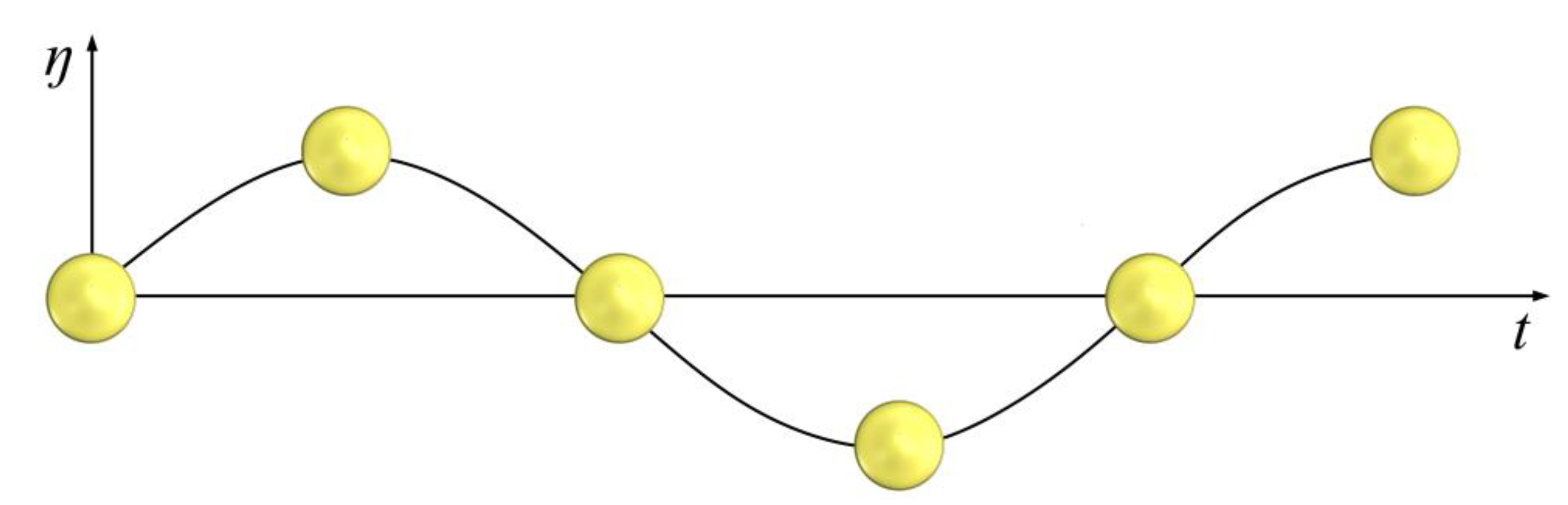
2.2. Motion Stability Analysis

According to Routh stability criterion [34], the discriminant of the AUH motion stability in the horizontal plane is:

$$N_r{Y}_v-N_v\left(Y_r-mV\right)>0$$

(12)

where $V$ is the initial velocity of the AUH. Dividing by $Y_v$ and $\left(Y_r-mV\right)$ results in

$$\frac{N_r}{Y_r-mV}-\frac{N_v}{Y_v}>0$$

(13)

This stability criterion can be expressed as a dimensionless parameter by introducing the length $L$ of the AUH, the initial velocity $V$ of the AUH, and the density $\rho$ of the fluid as follows

$$\frac{N_r^{\prime }}{(Y_r^{\prime }-m^{\prime })}-\frac{N_v^{\prime }}{Y_v^{\prime }}>0$$

(14)

Rewriting Equation (13) [17], the criterion ${\mathrm{G}}_{\mathrm{H}}$ in the horizontal plane is expressed as follows

$${\mathrm{G}}_{\mathrm{H}}=1-\frac{N_v^{\prime }\left(Y_r^{\prime }-m^{\prime }\right)}{Y_v^{\prime }{N}_r^{\prime }}$$

(15)

When ${\mathrm{G}}_{\mathrm{H}}$ is positive, the AUH has horizontal motion stability, and vice versa. A ${\mathrm{G}}_{\mathrm{H}}$ value greater than 1.0 indicates that the conventional AUV has high stability in the horizontal plane, which leads to poor maneuverability when the rudder is deflected [16]. However, since the AUH rotates through the cooperation of the propeller, a large ${\mathrm{G}}_{\mathrm{H}}$ value will not affect its maneuverability.

Similarly, according to the Routh stability criterion, the discriminant of the AUH motion stability in the vertical plane is [30]

$$\frac{M_q}{\left(Z_q+mV\right)}-\frac{M_w}{Z_w}>0$$

(16)

This stability criterion can be expressed as a dimensionless parameter by introducing the length $L$ of the AUH, the initial velocity $V$ of the AUH, and the density $\rho$ of the fluid as follows

$$\frac{M_q^{\prime }}{\left(Z_q^{\prime }+m^{\prime }\right)}-\frac{M_w^{\prime }}{Z_w^{\prime }}>0$$

(17)

Equation (18) can be expressed as an index used to determine the AUH motion stability in the vertical plane [30]:

$${\mathrm{G}}_{\mathrm{V}}=1-\frac{M_w^{\prime }\left(Z_q^{\prime }+m^{\prime }\right)}{Z_w^{\prime }{M}_q^{\prime }}$$

(18)

where, if ${\mathrm{G}}_{\mathrm{V}}$ is positive, the AUH has vertical motion stability, and vice versa. As the value of the index becomes greater than 1, the AUH becomes more dynamically stable. The AUH motion stability in the horizontal and vertical planes was verified in the RANS-based CFD study on the AUH motion stability using RNG $k-\epsilon$ turbulent models.

3. Numerical Simulation

3.1. Turbulence Model

CFD commercial software ANSYS Fluent is widely used to calculate the hydrodynamic performance of submersible vehicles [18,22,35,36] and provides a large number of turbulence models, among which the RANS model provides the most economical method for complex turbulent flow calculation. The two-equation model is the most widely used turbulence model in industrial CFD [29,37,38,39]. This model solves two transport equations and simulates Reynolds stress by the eddy viscosity method. The RNG $k-\epsilon$ model in ANSYS Fluent belongs to this kind of model, which solves the RANS equation.

$$\frac{\partial \rho }{\partial t}+\frac{\partial }{\partial x_i}\left(\rho u_i\right)=0$$

(19)

and

$$\begin{gathered} \frac{\partial }{\partial t}\left(\rho u_i\right)+\frac{\partial }{\partial x_j}\left(\rho u_i{u}_j\right) \\ =\frac{\partial p}{\partial x_i}+\frac{\partial }{\partial x_j}\left[\mu \left(\frac{\partial u_i}{\partial x_j}+\frac{\partial u_j}{\partial x_i}-\frac{2}{3}{\delta }_{ij}\frac{\partial u_l}{\partial x_l}\right)\right]+\frac{\partial }{\partial x_j}\left(-\rho \overline{u_i^{\prime }{u}_j^{\prime }}\right) \end{gathered}$$

(20)

The RNG $k-\epsilon$ model [40] is based on model transport equations for turbulent kinetic energy ($k$) and its dissipation rate ($\epsilon$), which are obtained from the following transport equations

$$\frac{\partial }{\partial t}\left(\rho k\right)+\frac{\partial }{\partial x_i}\left(\rho k{u}_i\right)=\frac{\partial }{\partial x_j}\left({\alpha }_k{\mu }_{eff}\frac{\partial k}{\partial x_j}\right)+G_k+G_b-\rho \epsilon -Y_M+S_k$$

(21)

and

$$\begin{gathered} \frac{\partial }{\partial t}\left(\rho \epsilon \right)+\frac{\partial }{\partial x_i}\left(\rho \epsilon u_i\right) \\ =\frac{\partial }{\partial x_j}\left({\alpha }_{\epsilon }{\mu }_{eff}\frac{\partial \epsilon }{\partial x_j}\right)+C_{1\epsilon }\frac{\epsilon }{k}\left(G_k+C_{3\epsilon }{G}_b\right)-C_{2\epsilon }\rho \frac{{\epsilon }^2}{k}-R_{\epsilon }+S_{\epsilon } \end{gathered}$$

(22)

In these equations, $G_k$ represents the generation of turbulent kinetic energy due to mean velocity gradients, and $G_b$ is the generation of turbulent kinetic energy due to buoyancy. $Y_M$ represents the contribution of the fluctuating dilatation in compressible turbulence to the overall dissipation rate. $C_{1\epsilon }, C_{2\epsilon }, C_{3\epsilon }$ are constants, and ${\sigma }_k$ and ${\sigma }_{\epsilon }$ are the turbulent Prandtl numbers for $k$ and $\epsilon$, respectively. The quantities ${\alpha }_k$ and ${\alpha }_{\epsilon }$ are the inverse effective Prandtl numbers for $k$ and $\epsilon$, respectively. $S_k$ and $S_{\epsilon }$ are user-defined source terms.

In their study on the hydrodynamic characteristics of the AUH with the original hull shape (HG1), Lin et al. [29] concluded that the results of the standard $k-\epsilon$ model underestimated the resistance and could not estimate the change in the side and lift force during the surge motion with zero angle of attack. Additionally, for the RNG $k-\epsilon$ model, a mesh number of over 10 million is necessary to capture the symmetric flow field around the symmetric AUH hull and predict the drag force with satisfactory accuracy [39]. Therefore, we also adopt the RNG $k-\epsilon$ model to capture the characteristics of the flow field around the hull with the number of meshes exceeding 10 million.

3.2. Mesh Configuration and Boundary Conditions in Flow Domain

Figure 4 shows the flow field domain for the simulation. The AUH (diameter of 1.5 $\mathrm{m}$) is placed in the domain with a length, width, and height of 15 m × 10 m × 10 m to reduce the wall effect [29], which is 5 m away from the inlet to ensure the full development of the flow field around the AUH. The overlapping mesh technology realized by the user-defined function (UDF) is adopted in the simulation. The main idea of the overlapping mesh method is to use a Cartesian right-angled mesh in the far background area of the computing domain and a body-fitted mesh on the object and each attachment. The data transfer between the two meshes is completed by interpolation to realize the mesh generation of the multi-attachment structure and the numerical simulation of complex motion [41]. As shown in Figure 4b, the ICEM software is used to divide the computational domain into a fixed background mesh for the flow domain and a fixed dynamic mesh on the AUH. Both types of meshes are hexahedral-structured meshes.

By using the RNG $k-\epsilon$ model and wall function, the boundary layer needs to be defined near the hull surface. Phillips et al. [16] proposed a method to calculate the thickness of the first layer of the boundary layer, $∆y=L{y}^{+}\sqrt{80}R{e}^{-\frac{13}{14}}, \delta =0.035LR{e}^{-\frac{13}{14}}$, where $Re$ is the Reynolds number defined as $VL/\nu$ ($\nu$ is the kinematic viscosity, and $L$ is the diameter of the AUH),$∆y$ is the first layer thickness, $\delta$ is the boundary layer thickness, and $20\le y^{+}\le 200$ [25]. Consequently, $\delta =5 \mathrm{mm}$ and $∆y=1 \mathrm{mm}$ are adopted in the simulation to make $y^{+}\approx 30$.

The no-slip condition is applied to the AUH hull and the side wall of the flowing domain. the inlet of the flow domain adopts the velocity inlet boundary condition (the velocity range is 0–2 $\mathrm{m}/\mathrm{s}$), and the outlet adopts the pressure outlet (0 $\mathrm{Pa}$). In order to study the evolution of resistance and moment with time, the unsteady model and different time steps from 0.01 s to 0.05 s are used for the calculation.

4. Results and Discussion

4.1. Hydrodynamic Analysis during Motions with Various Attitudes

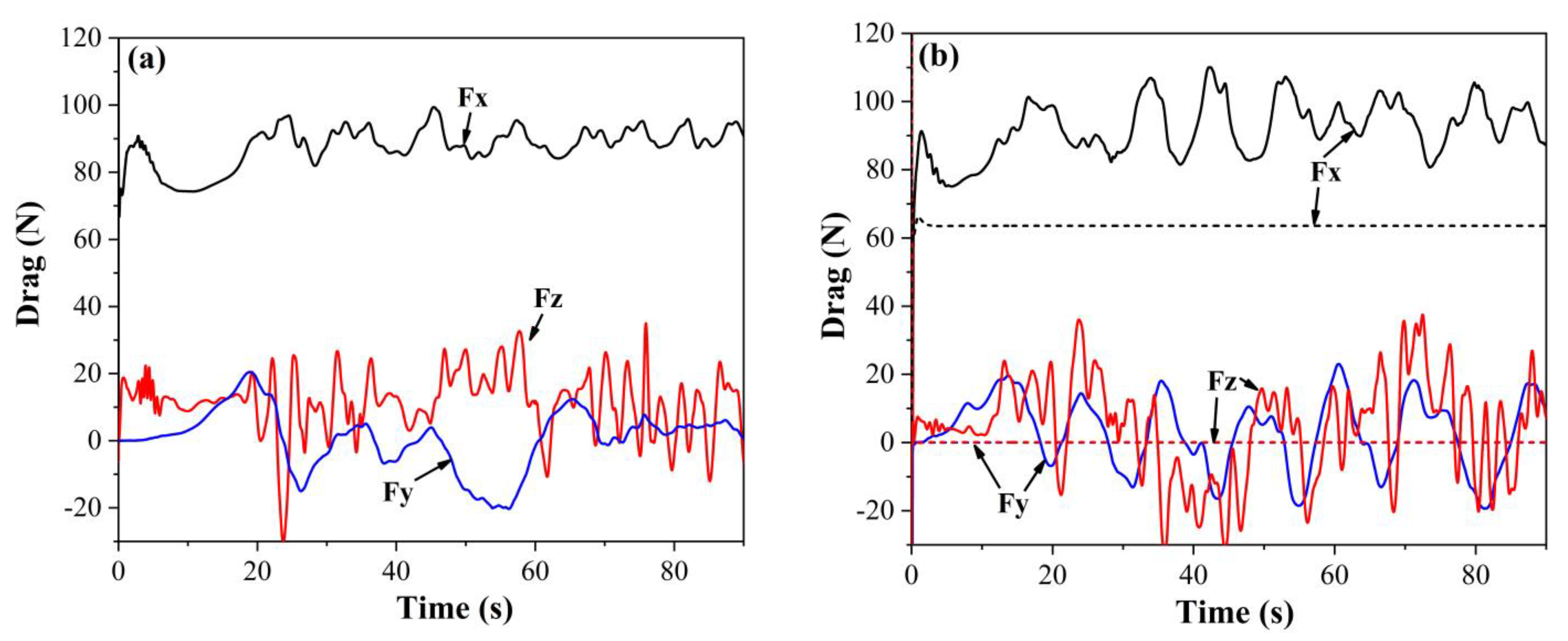
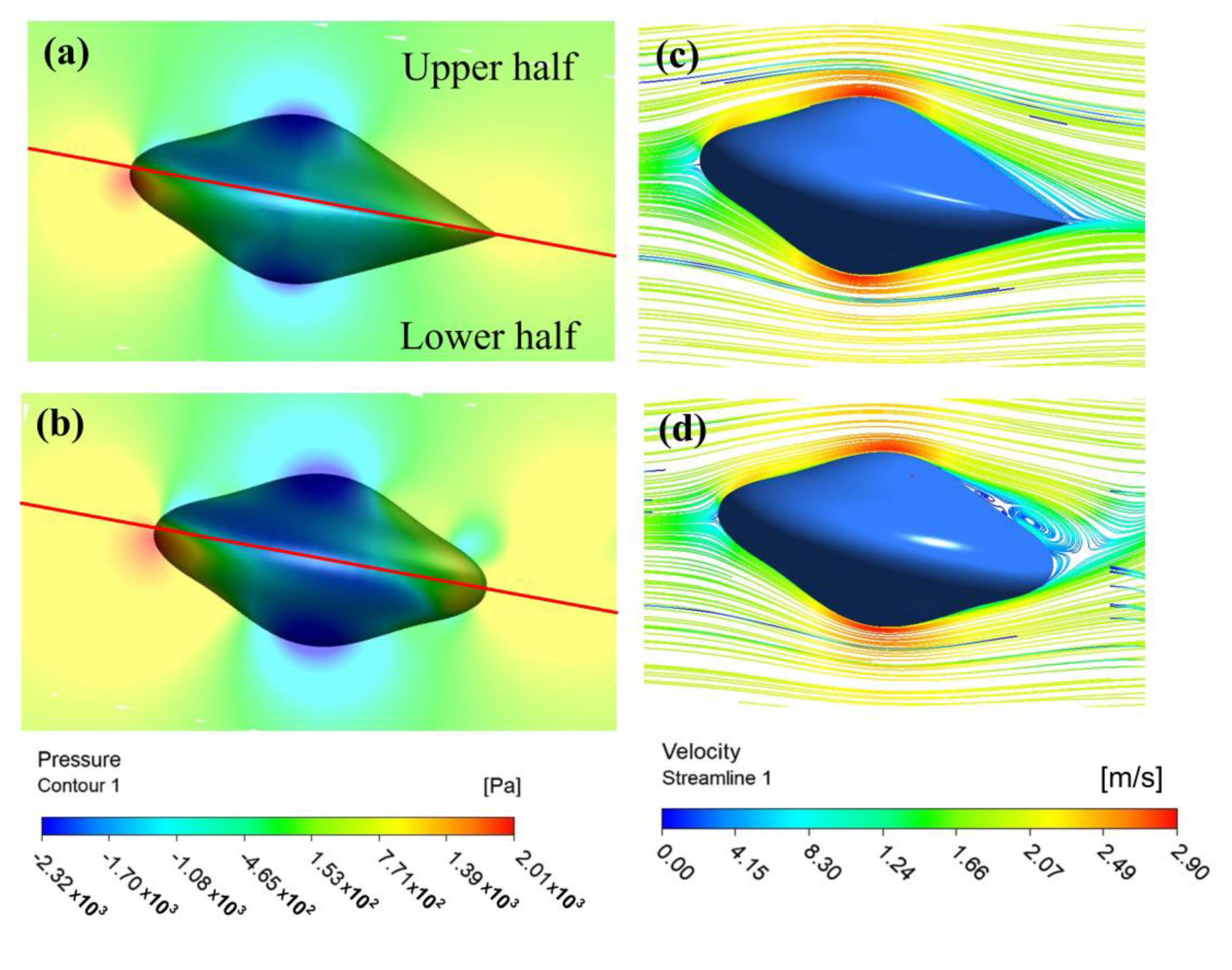
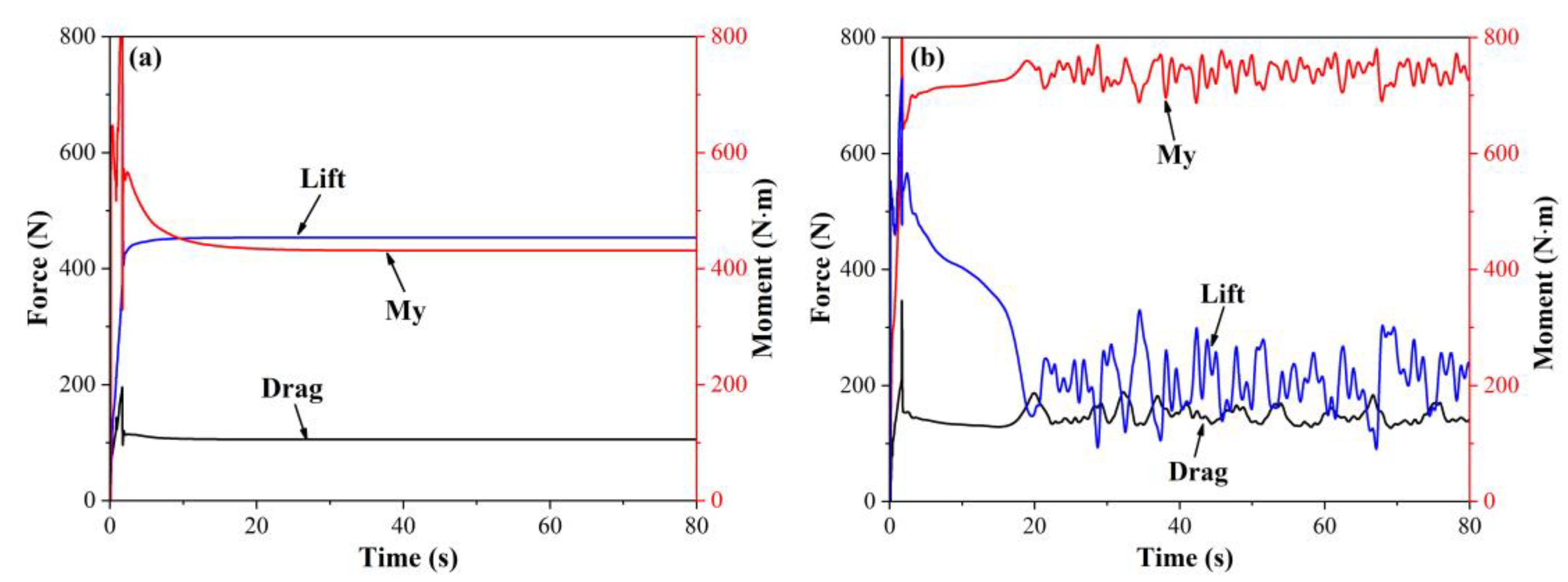
4.1.1. Hydrodynamic Analysis at Zero AOA

The hydrodynamic resistance of the fully disk-shaped HG1 moving 2 $\mathrm{m}/\mathrm{s}$ horizontally with zero angle of attack is calculated using the overlapping mesh method, which is compared to the simulation result with fixed meshes (non-overlapping meshes) [29]. As shown in Figure 5, the time-averaged value of $F_x$ calculated by the two kinds of meshes are both around 90 N, with an amplitude of pulsation of about 20 N, which is due to the periodic vortex shedding at the tail of the AUH. The average values of the lateral force $F_y$ and $F_z$ are close to zero, both with obvious fluctuation. Because the upstream area of the AUH in the heave direction is much larger than that in the sway direction, the amplitude of the lift force $F_z$ is larger than that of side $F_y$. Therefore, the overlapping-mesh method adopted can capture the correct characteristics of the flow field.

As shown in Figure 6a,b, for streamlines at the tail of the AUH hull, there is an obvious vortex area at the tail of HG1, which causes fluctuant drag and lift forces. By comparison, streamlines for HG3 are fairly smooth, indicating that HG3 has better hydrodynamic performance. Meanwhile, Figure 5b shows the hydrodynamic force of HG1 and HG3 at a speed of 2 $\mathrm{m}/\mathrm{s}$ with zero AOA. Compared to the resistance fluctuation of HG1, there is almost no resistance fluctuation of HG3. For HG3, the lateral force $F_y$ and $F_z$ are almost zero, and the time-averaged resistance of $F_x$ 29.3% is reduced by 20% compared to HG1.

4.1.2. Hydrodynamic Analysis with Non-Zero AOA

The AUH needs to maintain a stable straight motion between different height positions in order for better inspection near the seabed. The hydrodynamic performance of the AUH at a speed of 2 $\mathrm{m}/\mathrm{s}$ with the AOA varying from 0 to 30 degrees is investigated. As shown in Figure 7a, as the AOA increases, the projection area (along the upstream area) of the AUH on the $yoz$ plane shown in Figure 7b increases, so the drag resistance of HG1 and HG3 increases. When the AOA is less than 15 degrees, the increasing trend of resistance is small, and the resistance of HG3 is less than that of HG1. With the AOA exceeding 15 degrees, the increasing trend becomes more obvious, and the resistance of HG3 is greater than that of HG1. This is because after the tail of HG3 is elongated, its frontward area will be larger than that of HG1 after the AOA exceeds 15 degrees, which leads to an increase in pressure drag.

As shown in Figure 7c and Figure 8a,b, when the AUH moves with a non-zero AOA, the pressure distribution of the surrounding flow domain changes with respect to that with a zero AOA, which leads to a lift along the heave direction. When the AOA is less than 10 degrees, the lift of HG1 and HG3 is almost the same. When the AOA exceeds 15 degrees, the increasing trend of lift becomes obvious. Too much lift will increase the difficulty of the AUH motion control, so an AOA less than 15 degrees is conducive to the AUH seabed operation. The lift and drag forces applied on the AUH gives rise to a moment $M_y$, which makes the vessel pitch. As shown in Figure 7d. with the increase in the AOA, the pitching moment of HG1 and HG3 increases, and the pitching moment of HG3 is less than that of HG1, which shows that HG3 has better motion stability and anti-overturning ability.

In order to obtain the appropriate AOA of the vessel in a horizontal motion, the ratio of lift to drag is shown in Figure 7e. Ratios for HG1 and HG3 are both greater than 1, which first increase and then decrease, peaking at an angle of around 10 degrees. The ratio of HG3 is greater than that of HG1, which shows that HG3 has a better ability to change its vertical position. In the following, we analyze the hydrodynamic performance of HG1 and HG3 at an AOA of 10 degrees with the lift-to-drag ratio approaching maximum.

With a horizontal motion velocity of 2 $\mathrm{m}/\mathrm{s}$ and an AOA of 10 degrees, the pressure distribution of in the $xoz$ plane is shown in Figure 8a,b. At the heading part of the AUH hulls, the hydrodynamic pressure in the lower half is greater than that in the upper half, which is the origin of the lift, and the pressure contour is similar for the two hulls. At the rear part, it can be found that the pressure distribution of HG3 is smoother than that of HG1. As shown in Figure 8c, d, the vortex area with motion appears in the upper position of the tail, and the vortex area is significantly larger than that with a pure surge motion with zero AOA. It shows that when HG1 moves at the angle of attack, its hydrodynamic force and moment affect its stability more clearly. Accordingly, the temporal evolution of drag, lift, and overturning moment ($M_y$) at a velocity of 2 $\mathrm{m}/\mathrm{s}$ and an AOA of 10 degrees is shown in Figure 9. The time-averaged drag resistance and time-averaged overturning moment of HG3 are reduced by 27.5% and 38.4%, respectively, compared to HG1, which reduces the energy consumption of the AUH, and the reduction in the overturning moment can reduce the difficulty in motion control. The time-averaged lift of HG3 is 431.1 N, which is greater than that of HG1 (213.6 N). As the conclusion obtained from the analysis of streamlines above, the fluctuation in the resistance, lift, and moment of HG1 can be seen clearly in Figure 9, and the fluctuation amplitude of the lift is significantly greater than that of the other two. The larger lift fluctuation makes the angle of attack change continuously when the AUH moves, which affects the accuracy of the fixed-point tracking.

Through the hydrodynamic analysis of the AUH with the AOA, it can be concluded that the HG3 hull has significantly better drag reduction lift performance and anti-overturning stability compared to HG1.

4.2. Stability Analysis According to Route Stability Criterion

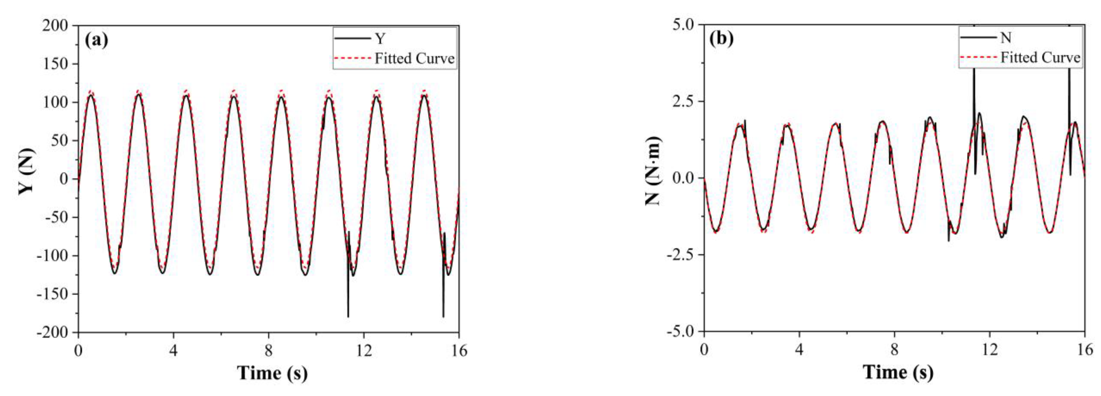
4.2.1. Numerical Simulation on Plane Motion Mechanism Test (PMM)

In this section, the overlapping mesh method through the UDF is adopted by the numerical simulation in the PMM test for the AUH hulls, and the obtained hydrodynamic force and hydrodynamic moment are fitted in MATLAB to solve the hydrodynamic coefficient. Based on the dimensionless hydrodynamic coefficient and the Routh criterion, the stability of the AUH horizontal and vertical motion is analyzed. In the simulation, the RNG $k-\epsilon$ turbulence model is used to simulate the AUH pure surge motion, pure sway motion, pure heave motion, pure pitch motion, pure roll motion, and pure yaw motion, and the time step is set to 0.015 s.

The pure sway motion of the AUH includes both uniform motion ($U=1\mathrm{m}/\mathrm{s}$) along the x-axis and harmonic oscillation along the y-axis (Figure 10). The equation of motion can be expressed as:

$$\{\begin{array}{c}\eta =0.04sin\omega t\\ v=\dot{\eta }=0.04\omega cos\omega t\\ \dot{v}=-0.04{\omega }^{2}sin\omega t\end{array}$$

(23)

where $\eta$ is the sway amplitude, $\omega =\pi$ is the frequency of harmonic motion.

Substituting the above equation into Equation (11), the hydrodynamic force $Y$ in the y-direction and the hydrodynamic moment $N$ around the z-axis can be obtained:

$$\{\begin{array}{c}Y=-0.04{\pi }^2{Y}_{\dot{v}}sin\pi t+0.04\pi Y_{v}cos\pi t+0.0016{\pi }^2{Y}_{v\left|v\right|}cos\pi t\left|cos\pi t\right|\\ N=-0.04{\pi }^2{N}_{\dot{v}}sin\pi t+0.04\pi N_{v}cos\pi t+0.0016{\pi }^2{N}_{v\left|v\right|}cos\pi t\left|cos\pi t\right|\end{array}$$

(24)

In the pure roll motion test, the AUH is restricted to move at a uniform velocity along the x-axis at velocity $U=1\mathrm{m}/\mathrm{s}$, meanwhile rotates harmoniously around the x-axis. The equation of motion can be expressed as:

$$\{\begin{array}{c}\varphi =\frac{0.04\omega }{U}sin\omega t\\ p=\dot{\varphi }=\frac{0.04{\omega }^2}{U}cos\omega t\\ \dot{p}=-\frac{0.04{\omega }^3}{U}sin\omega t\end{array}$$

(25)

where $\varphi$ is the roll angle, and $\omega =\pi$ is the frequency of harmonic motion. Substituting the above equation into Equation (11), the hydrodynamic force $Y$ in the y-direction and the hydrodynamic moment $K$ around the x-axis can be obtained:

$$\{\begin{array}{c}Y=-0.04{\pi }^3{Y}_{\dot{p}}sin\pi t+0.04{\pi }^2{Y}_{p}cos\pi t+0.0016{\pi }^4{Y}_{p\left|p\right|}cos\pi t\left|cos\pi t\right|\\ K=-0.04{\pi }^3{K}_{\dot{p}}sin\pi t+0.04{\pi }^2{K}_{p}cos\pi t+0.0016{\pi }^4{K}_{p\left|p\right|}cos\pi t\left|cos\pi t\right|\end{array}$$

(26)

The equations of the harmonic oscillation and the harmonic rotation motion in the other two directions are similar to the pure sway and the pure roll, so they will not be described again.

4.2.2. Hydrodynamic Coefficient Solution and Stability Analysis

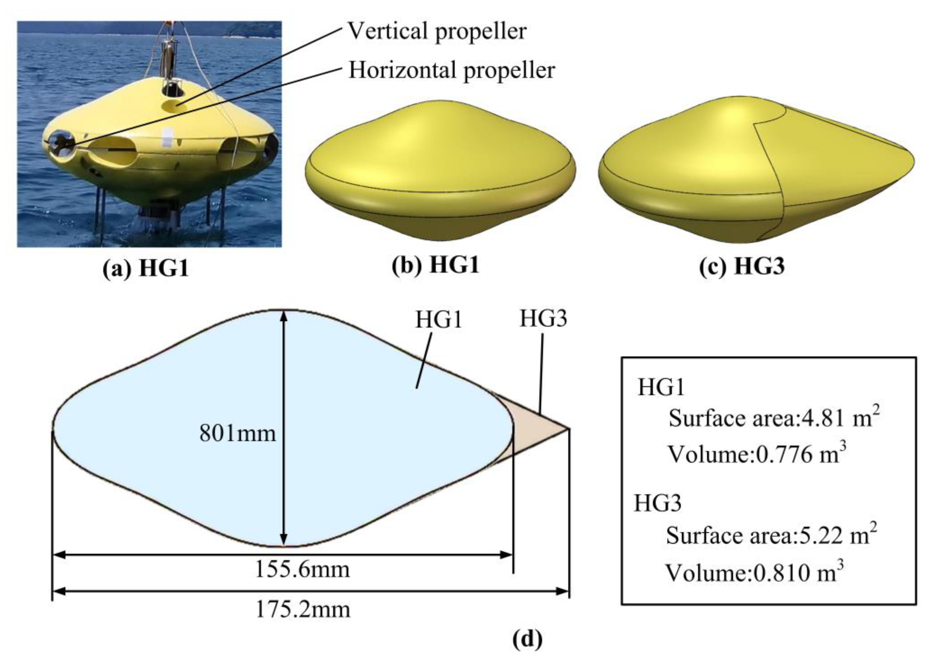
HG1

Taking pure sway and pure roll harmonic motion as an example, when HG1 sways according to the motion Equation (23), the changes in its hydrodynamic $Y$ in the y-direction and hydrodynamic moment $N$ around the z-axis with time are shown in Figure 11. The black solid line in the figure represents the CFD calculation results, and the red dotted line represents the curve fitted according to Equation (24). The dimensionless hydrodynamic coefficients calculated are shown in

Table 2. Dimensionless hydrodynamic coefficient of HG1.

Dimensionless Coefficient	Dimensionless Formula	Value	Dimensionless Coefficient	Dimensionless Formula	Value
$X_{\dot{u}}^{\prime }$	$\frac{X_{\dot{u}}}{1/2\rho L^3}$	−0.135	$X_u^{\prime }$	$\frac{X_u}{1/2\rho L^{2}U}$	−0.019
$X_{u\left|u\right|}^{\prime }$	$\frac{X_{u\left|u\right|}}{1/2\rho L^2}$	−0.033	$X_0^{\prime }$	$\frac{X_0}{1/2\rho L^2{U}^2}$	0.043
$Y_{\dot{v}}^{\prime }$	$\frac{Y_{\dot{v}}}{1/2\rho L^3}$	−0.173	$Y_v^{\prime }$	$\frac{Y_v}{1/2\rho L^{2}U}$	−0.096
$Y_{v\left|v\right|}^{\prime }$	$\frac{Y_{v\left|v\right|}}{1/2\rho L^2}$	0.117	$K_{\dot{v}}^{\prime }$	$\frac{K_{\dot{v}}}{1/2\rho L^4}$	0.056
$K_v^{\prime }$	$\frac{K_v}{1/2\rho L^{3}U}$	0.031	$K_{v\left|v\right|}^{\prime }$	$\frac{K_{v\left|v\right|}}{1/2\rho L^3}$	−0.070
$Z_{\dot{w}}^{\prime }$	$\frac{Z_{\dot{w}}}{1/2\rho L^3}$	0.555	$Z_w^{\prime }$	$\frac{Z_w}{1/2\rho L^{2}U}$	−0.499
$Z_{w\left|w\right|}^{\prime }$	$\frac{Z_{w\left|w\right|}}{1/2\rho L^2}$	0.096	$M_{\dot{w}}^{\prime }$	$\frac{M_{\dot{w}}}{1/2\rho L^4}$	−0.045
$M_w^{\prime }$	$\frac{M_w}{1/2\rho L^{3}U}$	−0.778	$M_{w\left|w\right|}^{\prime }$	$\frac{M_{w\left|w\right|}}{1/2\rho L^3}$	0.103
$Z_{\dot{q}}^{\prime }$	$\frac{Z_{\dot{q}}}{1/2\rho L^4}$	−0.021	$Z_q^{\prime }$	$\frac{Z_q}{1/2\rho L^{3}U}$	0.572
$Z_{q\left|q\right|}^{\prime }$	$\frac{Z_{q\left|q\right|}}{1/2\rho L^4}$	−0.154	$M_{\dot{q}}^{\prime }$	$\frac{M_{\dot{q}}}{1/2\rho L^5}$	−0.068
$M_q^{\prime }$	$\frac{M_q}{1/2\rho L^{4}U}$	−0.024	$M_{q\left|q\right|}^{\prime }$	$\frac{M_{q\left|q\right|}}{1/2\rho L^5}$	0.046
$N_{\dot{r}}^{\prime }$	$\frac{N_{\dot{r}}}{1/2\rho L^5}$	0.00018	$N_r^{\prime }$	$\frac{N_r}{1/2\rho L^{4}U}$	−0.0037
$N_{r\left|r\right|}^{\prime }$	$\frac{N_{r\left|r\right|}}{1/2\rho L^5}$	0.00026	$Y_{\dot{p}}^{\prime }$	$\frac{Y_{\dot{p}}}{1/2\rho L^4}$	0.034
$Y_p^{\prime }$	$\frac{Y_p}{1/2\rho L^{3}U}$	0.016	$Y_{p\left|p\right|}^{\prime }$	$\frac{Y_{p\left|p\right|}}{1/2\rho L^4}$	−0.0068
$K_{\dot{p}}^{\prime }$	$\frac{K_{\dot{p}}}{1/2\rho L^5}$	−0.046	$K_p^{\prime }$	$\frac{K_p}{1/2\rho L^{4}U}$	−0.021
$K_{p\left|p\right|}^{\prime }$	$\frac{K_{p\left|p\right|}}{1/2\rho L^5}$	0.0052	$m^{\prime }$	$\frac{m}{1/2\rho L^3}$	0.178

.

When HG1 rolls according to the motion described by Equation (25), the changes in hydrodynamic force $Y$ in the y-direction and hydrodynamic moment $N$ around the x-axis with time are shown in Figure 12. The hydrodynamic coefficients calculated are shown in Table 2.

According to the Routh criterion (Equation (3)), the horizontal motion stability coefficient index ${\mathrm{G}}_{\mathrm{H}}^{\mathrm{HG}1}=1.0$ and vertical motion stability index ${\mathrm{G}}_{\mathrm{V}}^{\mathrm{HG}1}=49.7$ of HG1 can be obtained. The result is significantly greater than that of a conventional AUV, which represents that the AUH is able to maintain motion stability in the vertical plane under deep-sea conditions. For a conventional underwater vehicle (AUV) with a rudder, a ${\mathrm{G}}_{\mathrm{V}}^{\mathrm{HG}1}$ value greater than 1 represents poor maneuverability [17]. However, since the AUH rotates through the cooperation of a propeller, a large ${\mathrm{G}}_{\mathrm{H}}$ value will not affect its maneuverability.

HG3

The hydrodynamic coefficients of HG3 calculated are shown in

Table 3. Dimensionless hydrodynamic coefficient of HG3.

Dimensionless Coefficient	Dimensionless Formula	Value	Dimensionless Coefficient	Dimensionless Formula	Value
$X_{\dot{u}}^{\prime }$	$\frac{X_{\dot{u}}}{1/2\rho L^3}$	−0.117	$X_u^{\prime }$	$\frac{X_u}{1/2\rho L^{2}U}$	0
$X_{u\left|u\right|}^{\prime }$	$\frac{X_{u\left|u\right|}}{1/2\rho L^2}$	−0.05	$X_0^{\prime }$	$\frac{X_0}{1/2\rho L^2{U}^2}$	0.027
$Y_{\dot{v}}^{\prime }$	$\frac{Y_{\dot{v}}}{1/2\rho L^3}$	−0.161	$Y_v^{\prime }$	$\frac{Y_v}{1/2\rho L^{2}U}$	−0.068
$Y_{v\left|v\right|}^{\prime }$	$\frac{Y_{v\left|v\right|}}{1/2\rho L^2}$	0.017	$K_{\dot{v}}$	$\frac{K_{\dot{v}}}{1/2\rho L^4}$	−0.002
$K_v$	$\frac{K_v}{1/2\rho L^{3}U}$	0.008	$K_{v\left|v\right|}$	$\frac{K_{v\left|v\right|}}{1/2\rho L^3}$	−0.00066
$Z_{\dot{w}}^{\prime }$	$\frac{Z_{\dot{w}}}{1/2\rho L^3}$	−0.658	$Z_w^{\prime }$	$\frac{Z_w}{1/2\rho L^{2}U}$	−1.540
$Z_{w\left|w\right|}^{\prime }$	$\frac{Z_{w\left|w\right|}}{1/2\rho L^2}$	0.288	$M_{\dot{w}}$	$\frac{M_{\dot{w}}}{1/2\rho L^4}$	0.0342
$M_w$	$\frac{M_w}{1/2\rho L^{3}U}$	−0.155	$M_{w\left|w\right|}$	$\frac{M_{w\left|w\right|}}{1/2\rho L^3}$	−0.056
$Z_{\dot{q}}$	$\frac{Z_{\dot{q}}}{1/2\rho L^4}$	0.003	$Z_q$	$\frac{Z_q}{1/2\rho L^{3}U}$	0.855
$Z_{q\left|q\right|}$	$\frac{Z_{q\left|q\right|}}{1/2\rho L^4}$	−0.141	$M_{\dot{q}}$	$\frac{M_{\dot{q}}}{1/2\rho L^5}$	−0.041
$M_q$	$\frac{M_q}{1/2\rho L^{4}U}$	−0.094	$M_{q\left|q\right|}$	$\frac{M_{q\left|q\right|}}{1/2\rho L^5}$	0.0269
$N_{\dot{r}}$	$\frac{N_{\dot{r}}}{1/2\rho L^5}$	−0.0005	$N_r$	$\frac{N_r}{1/2\rho L^{4}U}$	−0.00336
$N_{r\left|r\right|}$	$\frac{N_{r\left|r\right|}}{1/2\rho L^5}$	0.0014	$Y_{\dot{p}}$	$\frac{Y_{\dot{p}}}{1/2\rho L^4}$	0
$Y_p$	$\frac{Y_p}{1/2\rho L^{3}U}$	0	$Y_{p\left|p\right|}$	$\frac{Y_{p\left|p\right|}}{1/2\rho L^4}$	0
$K_{\dot{p}}$	$\frac{K_{\dot{p}}}{1/2\rho L^5}$	−0.0218	$K_p$	$\frac{K_p}{1/2\rho L^{4}U}$	−0.0194
$K_{p\left|p\right|}$	$\frac{K_{p\left|p\right|}}{1/2\rho L^5}$	0.000158

. According to the Routh criterion, the horizontal motion stability index and vertical motion stability index of HG3 can be calculated as ${\mathrm{G}}_{\mathrm{H}}^{\mathrm{HG}3}=1.0$, ${\mathrm{G}}_{\mathrm{V}}^{\mathrm{HG}3}=2.1$. Compared to the stability index ${\mathrm{G}}_{\mathrm{V}}^{\mathrm{HG}1}=49.7$ of HG1, the HG3 (${\mathrm{G}}_{\mathrm{V}}^{\mathrm{HG}3}=2.1$) motion stability in the vertical plane is slightly worse due to the fore–aft asymmetry of the HG3 shape, which causes it to produce a pitching moment when it moves vertically. In actual engineering applications, it is necessary to make the combination of two vertical propellers work to balance the pitching moment. Nevertheless, compared to the traditional torpedo-type AUV, the stability of the AUH (${\mathrm{G}}_{\mathrm{V}}^{\mathrm{HG}1}>1, {\mathrm{G}}_{\mathrm{V}}^{\mathrm{HG}3}>1$) on the vertical plane is much better [25].

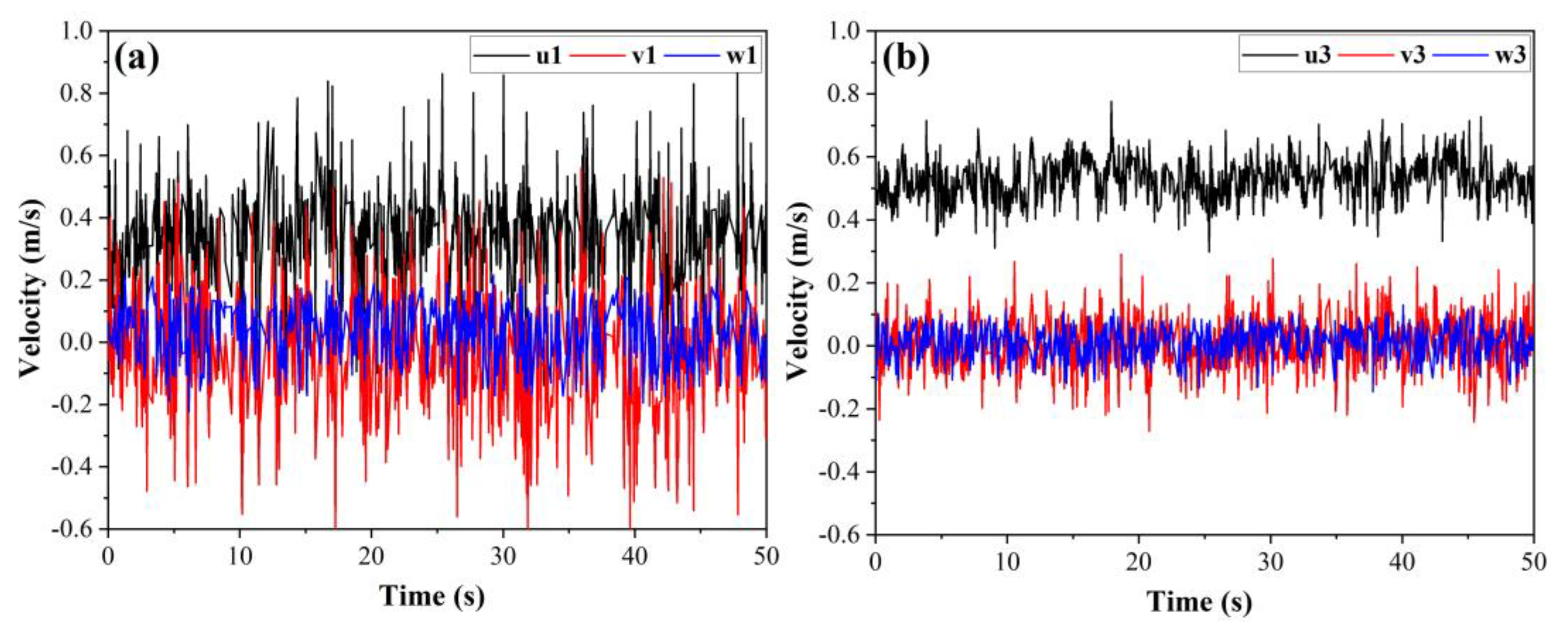
4.3. Experimental Validation with the Scale Model

A simple water channel experiment using the HG1 and HG3 models with a scale ratio of 1:10 was carried out, as shown in Figure 13, in order to verify the improvement in the hydrodynamic performance observed in the simulation during the surge motion of the AUH. The models were made of ultraviolet-light curable resin by 3D printing, and their surfaces were carefully polished to reduce roughness. The experiments were carried out in an open water channel with a rectangular cross-section of 400 × 500${\mathrm{mm}}^2$ and a water depth of 300 mm. The AUH model was installed at a water depth of 150 mm and in the middle of the side walls. The model was connected to an airfoil-shaped lever (airfoil profile naca0021) to minimize the additional disturbance to the flow field due to the presence of the lever. The average flow velocity at the “inflow boundary” or the background velocity ${\mathrm{u}}_{\mathrm{b}}$ is about 0.6 m/s. The Vectrino v1.18 (Nortek AS, Oslo, Norway) acoustic doppler velocimeter (ADV) was used to measure the flow velocity close to the rear part of the vessel, as shown in Figure 13. The flow velocity was measured at Location E on the x-axis, 172.2 mm apart horizontally from the nearest rear surface of the vessel.

As shown in Figure 14a, a large fluctuation in velocity is observed for the HG1 geometry. Compared with the flow velocity using HG3, the larger tail velocity fluctuations indicate that HG1 has a greater disturbance to the flow field at the rear, which reflects that the flow field close to the rear part of HG1 is more fluctuating and could result in the pulsation of drag force. Furthermore, for HG3, the time-averaged flow velocity along the x-direction (${\mathrm{u}}_3$ = 0.49 m/s) is greater than that of HG1 (${\mathrm{u}}_1$ = 0.35 m/s), from which it can be discerned that HG3 has a smaller hindering effect on the fluid, reflecting the smaller drag force for the HG3 hull. Consequently, the experimental results agree with the findings of the numerical simulation.

5. Conclusions

In this study, the six degree of freedom dynamic equation of the AUH space motion is derived. Based on the numerical simulation with the overlapping mesh method through the use of the UDF, the hydrodynamic performance of two AUH basic hulls (HG1 and HG3) is studied. When the AUH moves with an AOA less than 15 degrees and a speed of 2 $\mathrm{m}/\mathrm{s}$, HG3 has less resistance, greater lift, and a smaller overturning moment than HG1. This shows that HG3 has less energy loss and higher motion stability than HG1. In addition, with an AOA of about 10 degrees, HG1 and HG3 reach the maximum lift-to-drag ratio, which is always greater for HG3 than HG1. Additionally, HG3 has better hydrodynamic stability compared to HG3. The dimensionless hydrodynamic coefficients of the two models are deduced through a numerical PMM test based on the overlapping mesh method. According to the Routh stability criterion, the calculated stability index of horizontal and vertical motion of HG1 and HG3 (${\mathrm{G}}_{\mathrm{H}}^{\mathrm{HG}1}=1.0$, ${\mathrm{G}}_{\mathrm{V}}^{\mathrm{HG}1}=49.7$, ${\mathrm{G}}_{\mathrm{H}}^{\mathrm{HG}2}=1.0$,${\mathrm{G}}_{\mathrm{V}}^{\mathrm{HG}3}=2.1$) further shows that the AUH has better vertical motion stability than the torpedo-shaped AUV. The improvement in the hydrodynamic performance of the AUH with the HG3 hull is confirmed qualitatively by a simple water channel experiment on the scaled model.

References

1. Zhu, J.J.; Sun, Z.X.; Lian, S.M.; Yin, J.P.; Li, Z.G. Review on Cabled Seafloor Observatories in the World. J. Trop. Oceanogr. 2017, 36, 20–33. [Google Scholar]
2. Fenghua, L.; Yanguo, L.; Haibin, W.; Yonggang, G.; Fei, Z. Research Progress and Development Trend of Seafloor Observation Network. Bull. Chin. Acad. Sci. 2019, 34, 321–330. [Google Scholar]
3. Qi, S.-P.; Li, Y.-Z. A Review of the Development and Current Situation of Marine Environment Observation Technology and Instruments. Shandong Sci. 2019, 32, 21–29. [Google Scholar]
4. Bondaryk, J.E. Bluefin Autonomous Underwater Vehicles: Programs, Systems, and Acoustic Issues. J. Acoust. Soc. Am. 2004, 115, 2615. [Google Scholar] [CrossRef]
5. Hagen, P.E.; Storkersen, N.J.; Vestgard, K. HUGIN-Use of UUV Technology in Marine Applications. In Proceedings of the Oceans’ 99. MTS/IEEE. Riding the Crest into the 21st Century. Conference and Exhibition. Conference Proceedings (IEEE Cat. No. 99CH37008), Seattle, WA, USA, 13–16 September 1999; IEEE: New York, NY, USA, 1999; Volume 2, pp. 967–972. [Google Scholar]
6. Chance, T.; Kleiner, A.; Northcutt, J. The Autonomous Underwater Vehicle (AUV): A Cost-Effective Alternative to Deep-Towed Technology. Integr. Coast. Zone Manag. 2000, 2, 65–69. [Google Scholar]
7. Allen, B.; Stokey, R.; Austin, T.; Forrester, N.; Goldsborough, R.; Purcell, M.; von Alt, C. REMUS: A Small, Low Cost AUV; System Description, Field Trials and Performance Results. In Proceedings of the Oceans’ 97. MTS/IEEE Conference Proceedings, Halifax, NS, Canada, 6–9 October 1997; IEEE: New York, NY, USA, 1997; Volume 2, pp. 994–1000. [Google Scholar]
8. Pascoal, A.; Oliveira, P.; Silvestre, C.; Bjerrum, A.; Ishoy, A.; Pignon, J.-P.; Ayela, G.; Petzelt, C. MARIUS: An Autonomous Underwater Vehicle for Coastal Oceanography. IEEE Robot. Autom. Mag. 1997, 4, 46–59. [Google Scholar] [CrossRef]
9. Tanakitkorn, K.; Wilson, P.A.; Turnock, S.R.; Phillips, A.B. Depth Control for an Over-Actuated, Hover-Capable Autonomous Underwater Vehicle with Experimental Verification. Mechatronics 2017, 41, 67–81. [Google Scholar] [CrossRef] [Green Version]
10. Eriksen, C.C.; Osse, T.J.; Light, R.D.; Wen, T.; Lehman, T.W.; Sabin, P.L.; Ballard, J.W.; Chiodi, A.M. Seaglider: A Long-Range Autonomous Underwater Vehicle for Oceanographic Research. IEEE J. Ocean Eng. 2001, 26, 424–436. [Google Scholar] [CrossRef] [Green Version]
11. Sherman, J.; Davis, R.E.; Owens, W.B.; Valdes, J. The Autonomous Underwater Glider “Spray”. IEEE J. Ocean Eng. 2001, 26, 437–446. [Google Scholar] [CrossRef] [Green Version]
12. Stommel, H. The Slocum Mission. Oceanography 1989, 2, 22–25. [Google Scholar] [CrossRef]
13. Bachmayer, R.; Leonard, N.E.; Graver, J.; Fiorelli, E.; Bhatta, P.; Paley, D. Underwater Gliders: Recent Developments and Future Applications. In Proceedings of the 2004 International Symposium on Underwater Technology (IEEE Cat. No. 04EX869), Taipei, Taiwan, 20–23 April 2004; IEEE: New York, NY, USA, 2004; pp. 195–200. [Google Scholar]
14. Bettle, M.C.; Gerber, A.G.; Watt, G.D. Unsteady Analysis of the Six DOF Motion of a Buoyantly Rising Submarine. Comput. Fluids 2009, 38, 1833–1849. [Google Scholar] [CrossRef]
15. Du, X.; Wang, H.; Hao, C.; Li, X. Analysis of Hydrodynamic Characteristics of Unmanned Underwater Vehicle Moving Close to the Sea Bottom. Def. Technol. 2014, 10, 76–81. [Google Scholar] [CrossRef]
16. Phillips, A.; Furlong, M.; Turnock, S.R.B.T.-O. The Use of Computational Fluid Dynamics to Assess the Hull Resistance of Concept Autonomous Underwater Vehicles. In Proceedings of the OCEANS 2007-Europe, Aberdeen, UK, 18–21 June 2007; 2007; pp. 1–6. [Google Scholar]
17. Phillips, A.B.; Turnock, S.R.; Furlong, M. The Use of Computational Fluid Dynamics to Aid Cost-Effective Hydrodynamic Design of Autonomous Underwater Vehicles. Proc. Inst. Mech. Eng. Part M J. Eng. Marit. Environ. 2010, 224, 239–254. [Google Scholar] [CrossRef]
18. Salari, M.; Rava, A. Numerical Investigation of Hydrodynamic Flow over an AUV Moving in the Water-Surface Vicinity Considering the Laminar-Turbulent Transition. J. Mar. Sci. Appl. 2017, 16, 298–304. [Google Scholar] [CrossRef]
19. Sun, T.; Chen, G.; Yang, S.; Wang, Y.; Tan, H.; Zhang, L. Design and Optimization of a Bio-Inspired Hull Shape for AUV by Surrogate Model Technology. Eng. Appl. Comput. Fluid Mech. 2021, 15, 1057–1074. [Google Scholar] [CrossRef]
20. Wang, Z.; Liu, X.; Huang, H.; Chen, Y. Development of an Autonomous Underwater Helicopter with High Maneuverability. Appl. Sci. 2019, 9, 4072. [Google Scholar] [CrossRef] [Green Version]
21. Wu, L.; Li, Y.; Su, S.; Yan, P.; Qin, Y. Hydrodynamic Analysis of AUV Underwater Docking with a Cone-Shaped Dock under Ocean Currents. Ocean Eng. 2014, 85, 110–126. [Google Scholar] [CrossRef]
22. Jagadeesh, P.; Murali, K.; Idichandy, V.G. Experimental Investigation of Hydrodynamic Force Coefficients over AUV Hull Form. Ocean Eng. 2009, 36, 113–118. [Google Scholar] [CrossRef]
23. Mitra, A.; Panda, J.P.; Warrior, H.V. Experimental and Numerical Investigation of the Hydrodynamic Characteristics of Autonomous Underwater Vehicles over Sea-Beds with Complex Topography. Ocean Eng. 2020, 198, 106978. [Google Scholar] [CrossRef] [Green Version]
24. Mitra, A.; Panda, J.P.; Warrior, H.V. The Effects of Free Stream Turbulence on the Hydrodynamic Characteristics of an AUV Hull Form. Ocean Eng. 2019, 174, 148–158. [Google Scholar] [CrossRef] [Green Version]
25. Chen, C.-W.; Jiang, Y.; Huang, H.-C.; Ji, D.-X.; Sun, G.-Q.; Yu, Z.; Chen, Y. Computational Fluid Dynamics Study of the Motion Stability of an Autonomous Underwater Helicopter. Ocean Eng. 2017, 143, 227–239. [Google Scholar] [CrossRef]
26. Chen, C.-W.; Chen, Y.; Cai, Q.-W. Hydrodynamic-Interaction Analysis of an Autonomous Underwater Hovering Vehicle and Ship with Wave Effects. Symmetry 2019, 11, 1213. [Google Scholar] [CrossRef] [Green Version]
27. Chen, C.-W.; Lu, Y.-F. Computational Fluid Dynamics Study of Water Entry Impact Forces of an Airborne-Launched, Axisymmetric, Disk-Type Autonomous Underwater Hovering Vehicle. Symmetry 2019, 11, 1100. [Google Scholar] [CrossRef] [Green Version]
28. An, X.; Chen, Y.; Huang, H. Parametric Design and Optimization of the Profile of Autonomous Underwater Helicopter Based on Nurbs. J. Mar. Sci. Eng. 2021, 9, 668. [Google Scholar] [CrossRef]
29. Lin, Y.; Huang, Y.; Zhu, H.; Huang, H.; Chen, Y. Simulation Study on the Hydrodynamic Resistance and Stability of a Disk-Shaped Autonomous Underwater Helicopter. Ocean Eng. 2021, 219, 108385. [Google Scholar] [CrossRef]
30. Minnick, L.M. A Parametric Model for Predicting Submarine Dynamic Stability in Early Stage Design. Master’s Thesis, Virginia Tech, Blacksburg, VA, USA, 2006. [Google Scholar]
31. Woolsey, C.A. Review of Marine Control. Systems: Guidance, Navigation, and Control of Ships, Rigs and Underwater Vehicles. J. Guid. Control Dyn. 2005, 28, 574–575. [Google Scholar] [CrossRef]
32. Chen, C.W.; Kouh, J.S.; Tsai, J.F. Maneuvering Modeling and Simulation of AUV Dynamic Systems with Euler-Rodriguez Quaternion Method. China Ocean Eng. 2013, 27, 403–416. [Google Scholar] [CrossRef]
33. Chen, C.W.; Kouh, J.S.; Tsai, J.F. Modeling and Simulation of an AUV Simulator with Guidance System. IEEE J. Ocean. Eng. 2013, 38, 211–225. [Google Scholar] [CrossRef]
34. Fossen, T.I. Marine Control Systems–Guidance. Navigation, and Control of Ships, Rigs and Underwater Vehicles; Marine Cybernetics: Trondheim, Norway, 2002. [Google Scholar]
35. Divsalar, K. Improving the Hydrodynamic Performance of the SUBOFF Bare Hull Model: A CFD Approach. Acta Mech. Sin. 2020, 36, 44–56. [Google Scholar] [CrossRef]
36. Gao, T.; Wang, Y.; Pang, Y.; Cao, J. Hull Shape Optimization for Autonomous Underwater Vehicles Using CFD. Eng. Appl. Comput. Fluid Mech. 2016, 10, 599–607. [Google Scholar] [CrossRef] [Green Version]
37. Hu, J.M.; Zhang, Y.R.; Xu, G.; Zhang, Z.Q. Numerical Analysis of Hydrodynamic Performance of Biomimetic Flapping Foils Based on the RANS Method. J. Intell. Fuzzy Syst. 2020, 38, 7553–7562. [Google Scholar] [CrossRef]
38. Rattanasiri, P.; Wilson, P.A.; Phillips, A.B. Numerical Investigation of a Pair of Self-Propelled AUVs Operating in Tandem. Ocean Eng. 2015, 100, 126–137. [Google Scholar] [CrossRef] [Green Version]
39. Shojaeefard, M.H.; Khorampanahi, A.; Mirzaei, M. RANS Study of Strouhal Number Effects on the Stability Derivatives of an Autonomous Underwater Vehicle. J. Braz. Soc. Mech. Sci. Eng. 2018, 40, 1–11. [Google Scholar] [CrossRef]
40. Yakhot, V.; Orszag, S.A. Renormalization Group Analysis of Turbulence. I. Basic Theory. J. Sci. Comput. 1986, 1, 3–51. [Google Scholar] [CrossRef]
41. Sitaraman, J.; Floros, M.; Wissink, A.; Potsdam, M.; Sankaran, V. Parallel Unsteady Overset Mesh Methodology for a Multi-Solver Paradigm with Adaptive Cartesian Grids. In Proceedings of the 26th AIAA Applied Aerodynamics Conference, Honolulu, HI, USA, 18–21 August 2008. [Google Scholar]
Figure 1. Submarine mobile observation network.
Jmse 10 00060 g001
Figure 2. (a) AUH during a trial in the lake; (b) AUH with an original disk-shaped hull (HG1), (c) with an improved fore–aft asymmetric hull (HG3), and (d) profiles and geometric parameters of the HG1 and HG3.
Jmse 10 00060 g002
Figure 3. Coordinate system definition.
Jmse 10 00060 g003
Figure 4. (a) Layout and boundary conditions of simulation domain; (b) hexahedral-structured meshes.
Jmse 10 00060 g004
Figure 5. Evolution of the three force components with time at mesh number of about 11 million using the RNG k ε turbulence model: (a) non-overlapping mesh for HG1 and (b) overlapping mesh; solid lines for HG1 and dashed lines for HG3.
Jmse 10 00060 g005
Figure 6. Streamlines of AUH in x o z plane at a velocity of 2 m / s and an AOA of 10 degrees (a) for HG3 and (b) for HG1.
Jmse 10 00060 g006
Figure 7. (a) Projection area (along upstream area) of HG1 on the y o z plane and simulated variations of the drag, lift, and moment and drag-to-lift ratio as a function of the angle of attack (AOA). (b) drag, (c) lift, (d) moment, (e) lift to drag ratio.
Jmse 10 00060 g007
Figure 8. Pressure distribution and streamlines of AUH in x o z plane at a velocity of 2 m / s and an AOA of 10 degrees (a,c) for HG3 (b,d) for HG1.
Jmse 10 00060 g008
Figure 9. Simulated variations of the drag, lift, and moment as a function of time: (a) HG3; (b) HG1.
Jmse 10 00060 g009
Figure 10. Diagram of the pure sway motion of AUH.
Jmse 10 00060 g010
Figure 11. Simulation results of harmonic sway are fitted by MATLAB: (a) transverse force; (b) yaw moment.
Jmse 10 00060 g011
Figure 12. Simulation results of harmonic sway fitted by MATLAB: (a) transverse force; (b) roll moment.
Jmse 10 00060 g012
Figure 13. Schematic diagram of experimental system and the locations (E) for the flow velocity investigation close to the rear surface of the vessel.
Jmse 10 00060 g013
Figure 14. Temporal evolution of the flow velocity for HG1 and HG3 geometries at Location E, respectively, determined by the water channel experiment (a) for HG1 and (b) for HG3.
Jmse 10 00060 g014