
Water and Salt Transports in the Hengsha Channel of Changjiang Estuary


Abstract
:1. Introduction
2. Methods
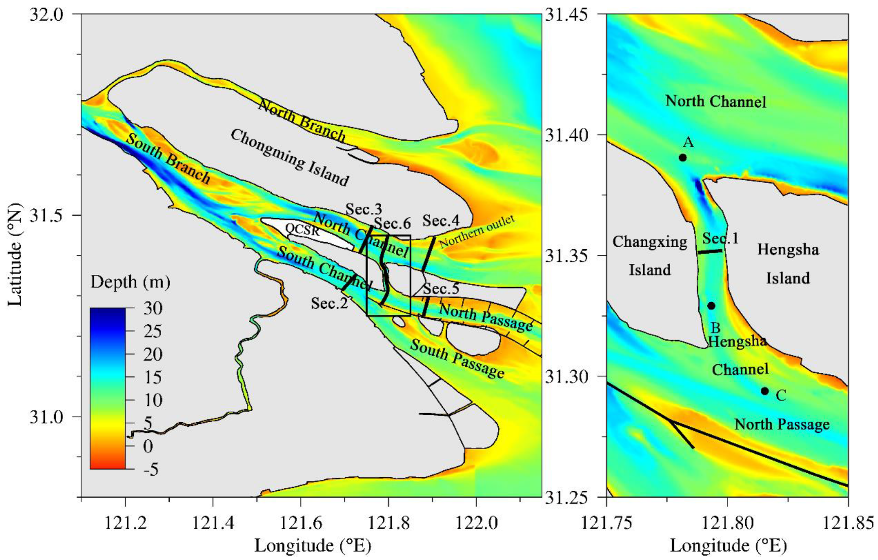
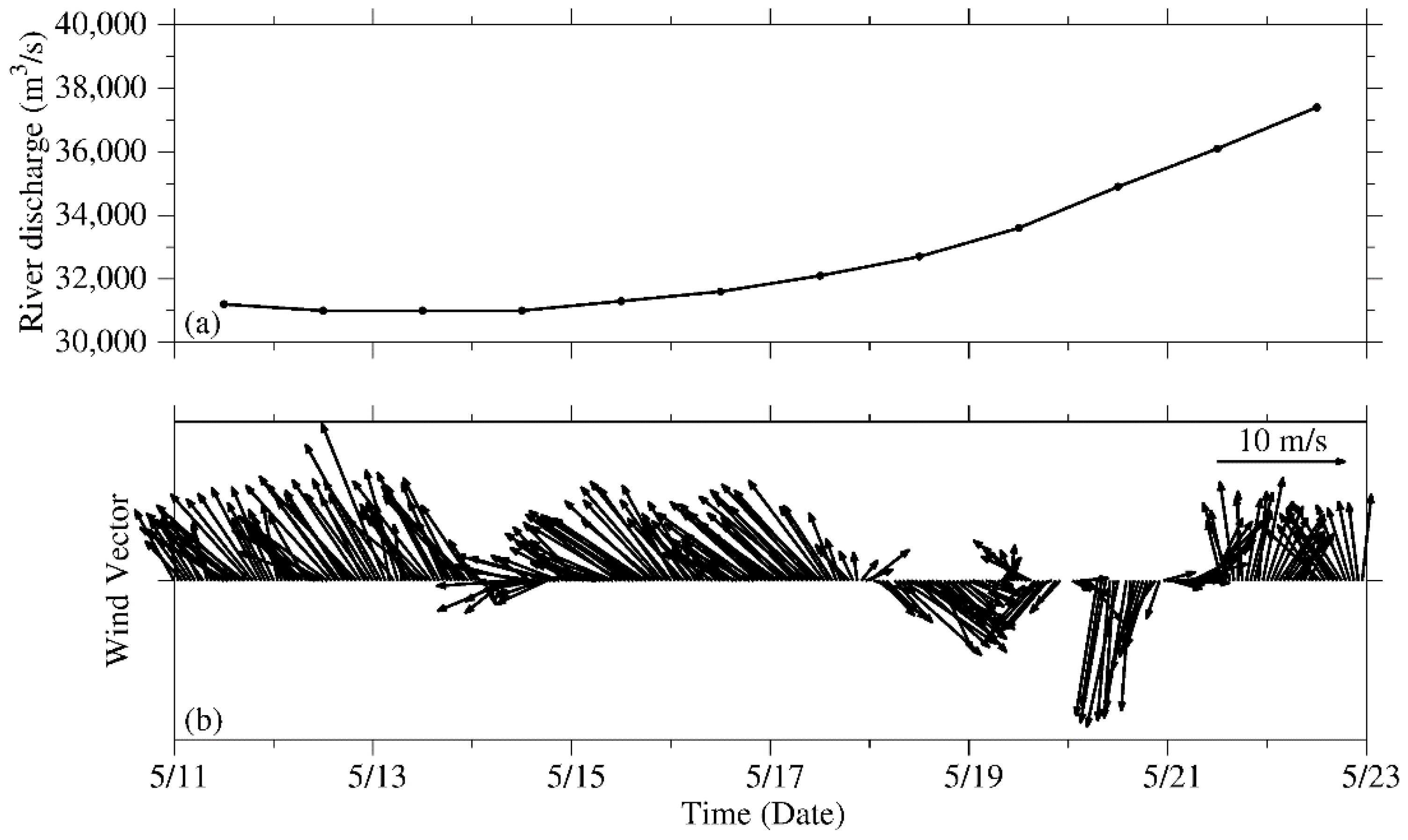
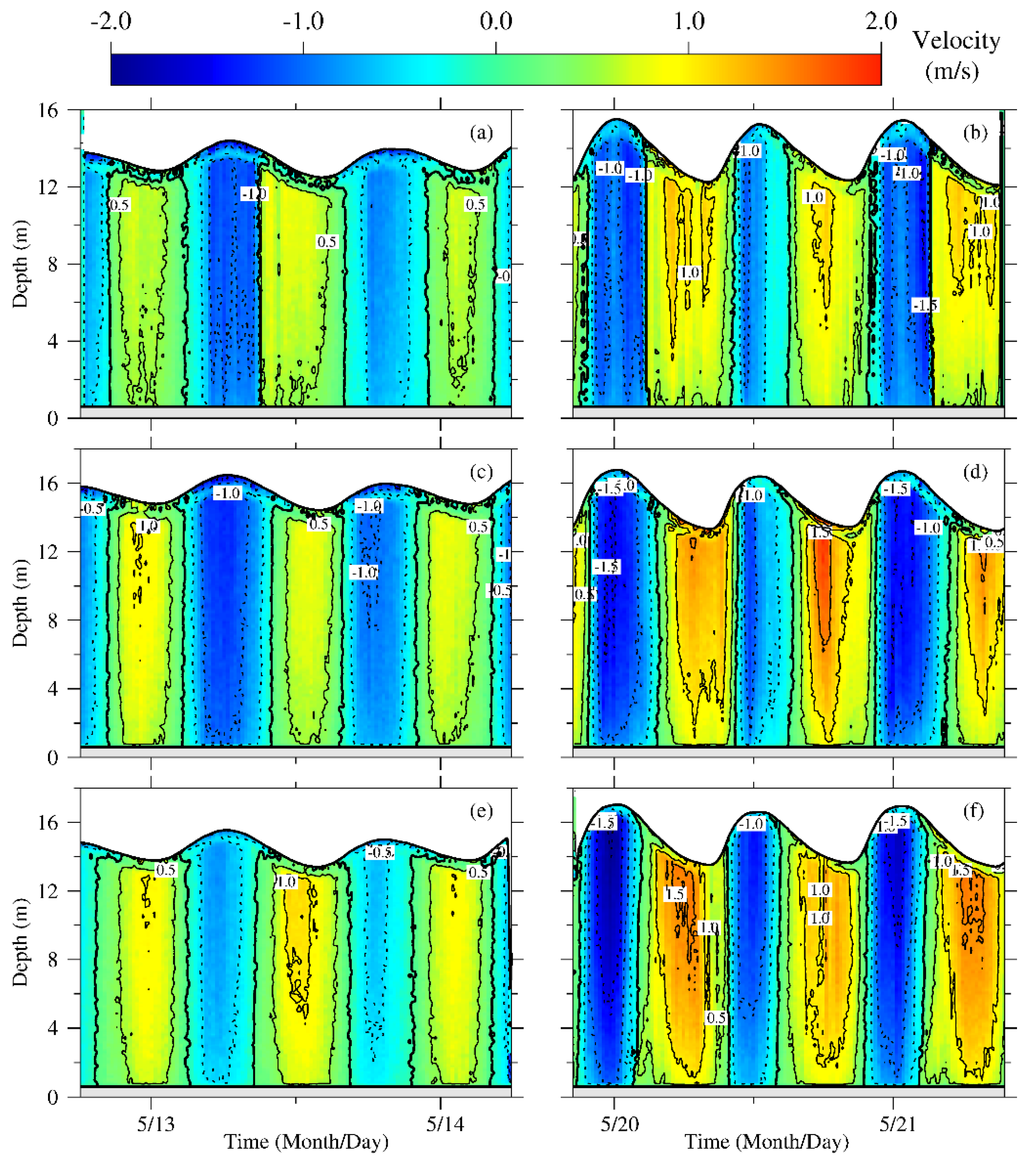
2.1. Observations
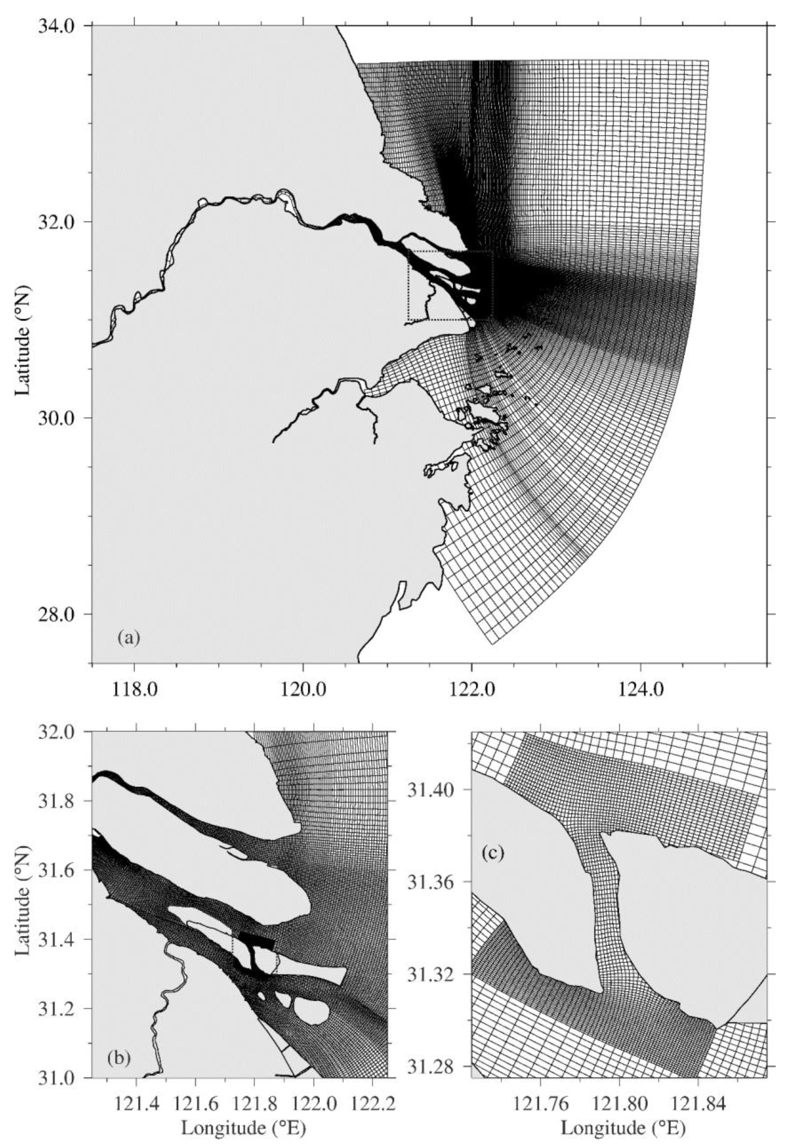
2.2. Numerical Model Configuration
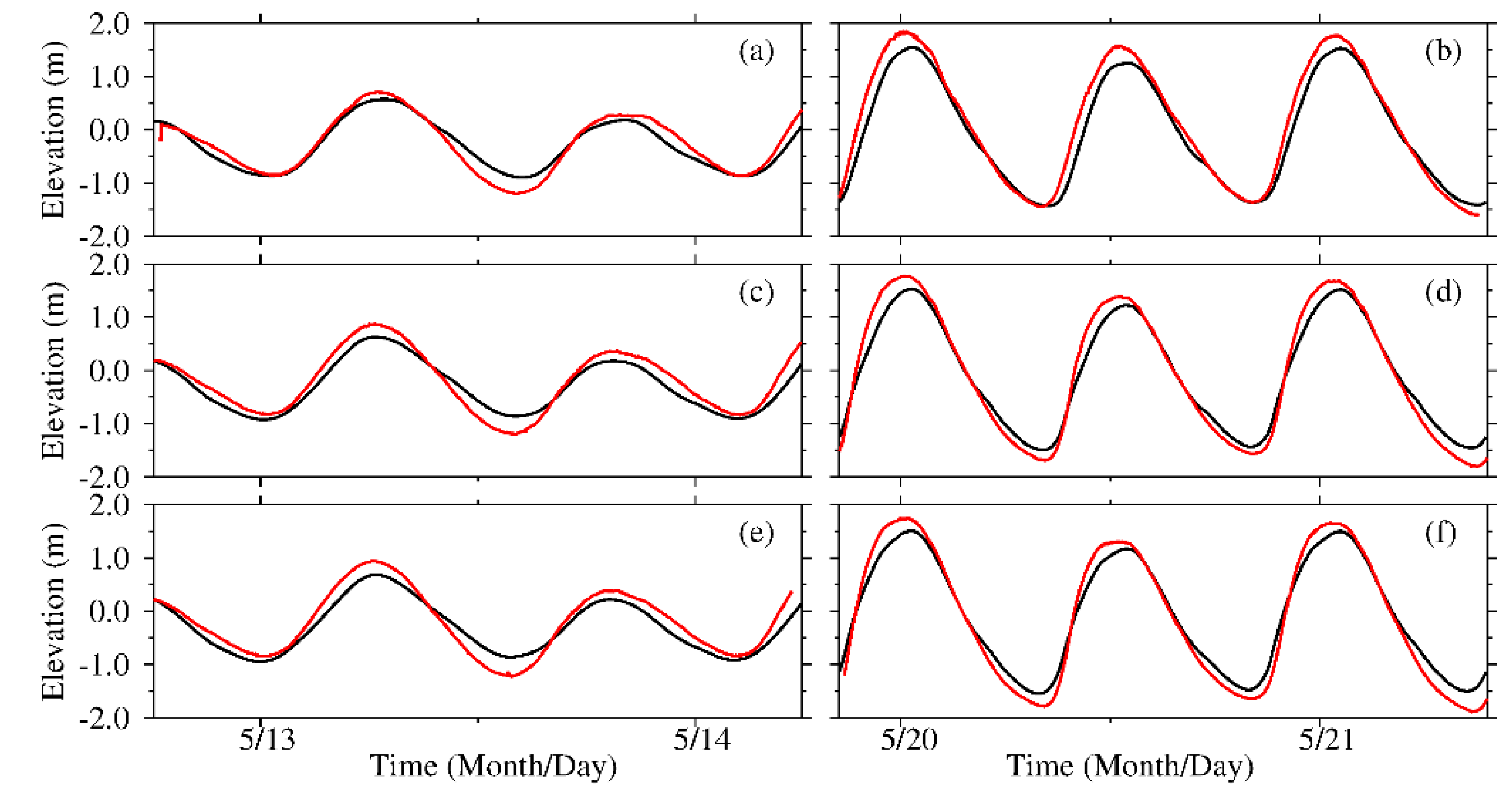
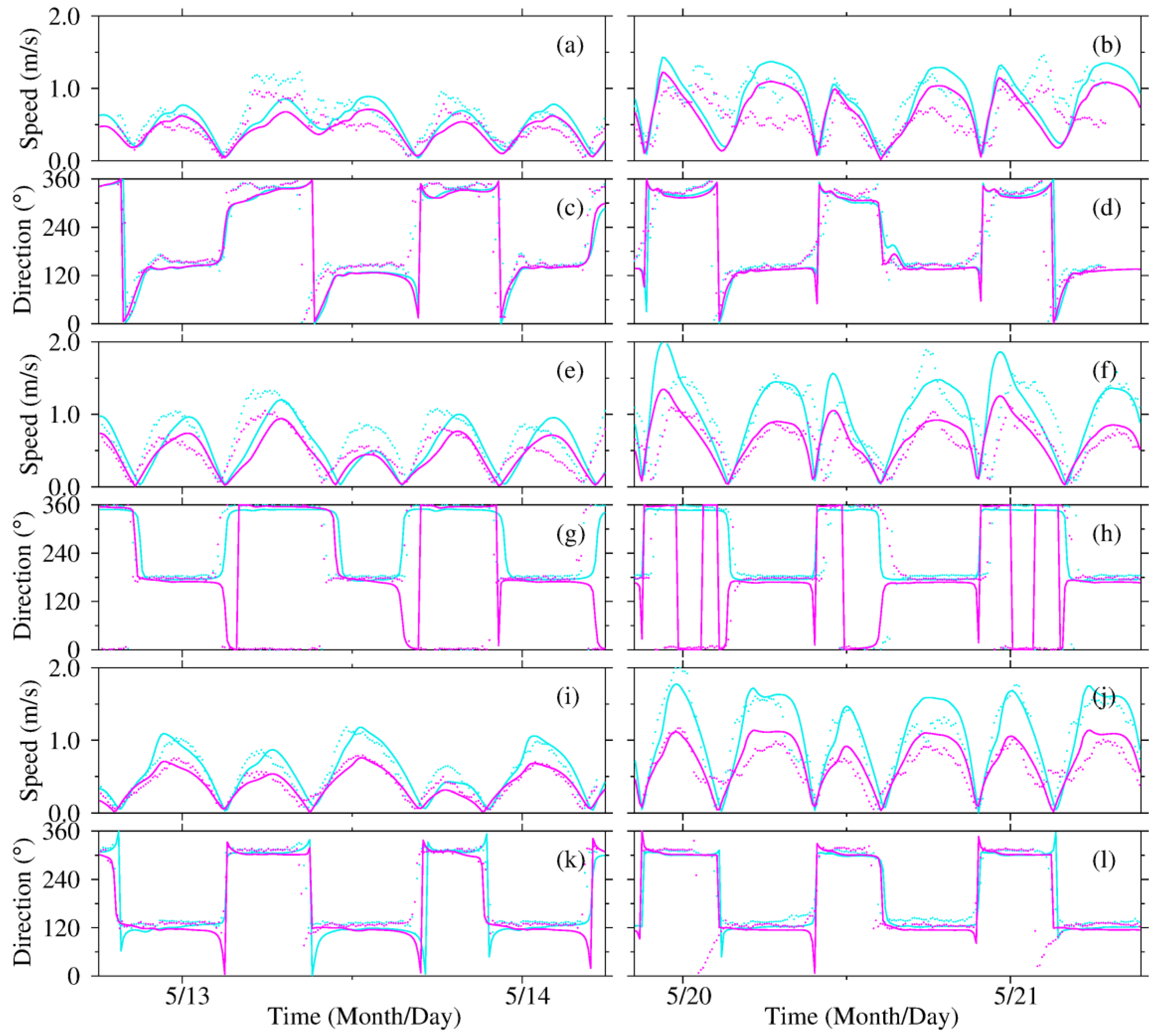
2.3. Model Validation
2.4. Residual Transport of Water and Salt
2.5. Numerical Experiments
3. Results
3.1. In the Realistic Case
3.2. In the Climatic Case
4. Discussion
4.1. Tides
4.2. River Discharge
4.3. Wind
4.4. Tide and River Discharge Interactions
5. Conclusions
Author Contributions
Funding
Institutional Review Board Statement
Informed Consent Statement
Data Availability Statement
Acknowledgments
Conflicts of Interest
References
- Woodroffe, C.; Nicholls, R.; Saito, Y.; Chen, Z.; Goodbred, S. Landscape Variability and the Response of Asian Megadeltas to Environmental Change. In Global Change and Integrated Coastal Management; Springer: Dordrecht, The Netherlands, 2006; pp. 277–314. [Google Scholar]
- Kondratyev, K.Y.; Pozdnyakov, D. Land-ocean interactions in the coastal zone: The LOICZ project. Il Nuovo Cimento C 1996, 19, 339–354. [Google Scholar] [CrossRef]
- Perillo, G. New geodynamic definition of estuaries. Rev. Geophys. 1989, 31, 281–287. [Google Scholar]
- Pritchard, D.W. The dynamic structure of a coastal plain estuary. J. Mar. Res. 1956, 15, 33–42. [Google Scholar]
- Pritchard, D.W. A study of the salt balance in a coastal plain estuary. J. Mar. Res. 1954, 13, 133–144. [Google Scholar]
- Pritchard, D.W. Salinity distribution and circulation in the Chesapeake Bay estuarine system. J. Mar. Res. 1952, 13, 133–144. [Google Scholar]
- Blumberg, A.F. The influence of density variations on estuarine tides and circulations. Estuar. Coast. Mar. Sci. 1978, 6, 209–215. [Google Scholar] [CrossRef]
- Chambers, L.; Osborne, T.; Reddy, K. Effect of salinity-altering pulsing events on soil organic carbon loss along an intertidal wetland gradient: A laboratory experiment. Biogeochemistry 2013, 115, 363–383. [Google Scholar] [CrossRef]
- Festa, J.F.; Hansen, D.V. A two-dimensional numerical model of estuarine circulation: The effects of altering depth and river discharge. Estuar. Coast. Mar. Sci. 1976, 4, 309–323. [Google Scholar] [CrossRef]
- Frankenberger, W.; Bingham, F. Influence of Salinity on Soil Enzyme Activities. Soil Sci. Soc. Am. J. 1982, 46, 1173–1177. [Google Scholar] [CrossRef]
- Hansen, F. Turbidity maxima in partially mixed estuaries: A two-dimensional numerical model. Estuar. Coast. Mar. Sci. 1978, 7, 347–359. [Google Scholar]
- Neubauer, S. Ecosystem Responses of a Tidal Freshwater Marsh Experiencing Saltwater Intrusion and Altered Hydrology. Estuaries Coasts 2013, 36, 491–507. [Google Scholar] [CrossRef]
- Weston, N.; Dixon, R.; Joye, S. Ramifications of increased salinity in tidal freshwater sediments: Geochemistry and microbial pathways of organic matter mineralization. J. Geophys. Res. 2006, 111, G1009. [Google Scholar] [CrossRef] [Green Version]
- Lerczak, J.; Geyer, W. Mechanisms Driving the Time-Dependent Salt Flux in a Partially Stratified Estuary. J. Phys. Oceanogr. 2006, 36, 2296–2311. [Google Scholar] [CrossRef] [Green Version]
- Tian, X. A Study on Turbidity Maximun in Lingdingyang Estuary of the Pearl River. Trop. Oceanol. 1986, 5, 27–35, (In Chinese with English abstart). [Google Scholar]
- Officer, C. Physical dynamics of estuarine suspended sediments. Mar. Geol. 1981, 40, 1–14. [Google Scholar] [CrossRef]
- Geyer, W.R. Contemporary Issues in Estuarine Physics: Estuarine salinity structure and circulation. Contemp. Issues Estuar. Phys. 2010, 12, 26. [Google Scholar]
- Wu, H.; Zhu, J.R. Analysis of the transport mechanism of the saltwater spilling over from the North Branch in the Changjiang Estuary in China. Acta Oceanol. Sin. 2007, 29, 17–25. [Google Scholar]
- Geyer, W.R.; Nepf, H. Tidal pumping of salt in a moderately stratified estuary. In Buoyancy Effects on Coastal and Estuarine Dynamics; American Geophysical Union (AGU): Washington, DC, USA, 1996. [Google Scholar]
- Geyer, W.R.; Smith, J.D. Shear Instability in a Highly Stratified Estuary. J. Phys. Oceanogr. 1987, 17, 1668–1679. [Google Scholar] [CrossRef] [Green Version]
- Liu, J. The Pearl River Delta Sixianjiao Channel, Tianhe Node Split Ratio on Law. Pearl River 2016, 37, 15–20, (In Chinese with English abstart). [Google Scholar]
- Ying, Z.F.; Chen, Z.Y.; Chen, S.G. A Discussion on Evolution of Sixian-jiao Channel and Its Regulation of the Water and Sediment. Acta Sci. Nat. Univ. Sunyatseni 1984, 4, 130–137, (In Chinese with English abstart). [Google Scholar]
- Shaha, D.C.; Cho, Y. Salt Plug Formation Caused by Decreased River Discharge in a Multi-channel Estuary. Sci. Rep. 2016, 6, 27176. [Google Scholar] [CrossRef]
- Mirza, M. The Ganges Water Diversion: Environmental Effects and Implications; Kliwer Academic Publishers (Springer): Dordrecht, The Netherlands, 2004. [Google Scholar]
- Mirza, M. RESEARCH: Diversion of the Ganges Water at Farakka and Its Effects on Salinity in Bangladesh. Environ. Manag. 1998, 22, 711–722. [Google Scholar] [CrossRef]
- Lacy, J.; Stacey, M.; Burau, J.; Monismith, S. Interaction of lateral baroclinic forcing and turbulence in an estuary. J. Geophys. Res. 2003, 108. [Google Scholar] [CrossRef]
- Walters, R.; Cheng, R.; Conomos, T. Time scales of circulation and mixing processes of San Francisco Bay waters. Hydrobiologia 1985, 129, 13–36. [Google Scholar] [CrossRef]
- Swinkels, C.; Jeuken, C.; Wang, Z.B.; Nicholls, R. Presence of Connecting Channels in the Western Scheldt Estuary. J. Coast. Res. 2009, 25, 627–640. [Google Scholar] [CrossRef]
- Jeuken, M.C.J.L. On the Morphologic Behaviour of Tidal Channels in the Westerschelde Estuary. Ned. Geogr. Stud. 2000, 79, 1–378. [Google Scholar]
- Shen, H.T.; Mao, Z.C.; Zhu, J.R. Salwater Intrusion in the Changjiang Estuary; China Ocean Press: Beijing, China, 2003; (In Chinese with English Abstract). [Google Scholar]
- Lyu, H.; Zhu, J. Impact of the bottom drag coefficient on saltwater intrusion in the extremely shallow estuary. J. Hydrol. 2018, 557, 838–850. [Google Scholar] [CrossRef]
- Wu, H.; Zhu, J.R.; Chen, B.; Chen, Y. Quantitative relationship of runoff and tide to saltwater spilling over from the North Branch in the Changjiang Estuary: A numerical study. Estuar. Coast. Shelf Sci. 2006, 69, 125–132. [Google Scholar] [CrossRef]
- Li, L.; Zhu, J.R.; Wu, H.; Wang, B. A numerical study on water diversion ratio of the Changjiang (Yangtze) estuary in dry season. Chin. J. Oceanol. Limn. 2010, 28, 700–712. [Google Scholar] [CrossRef]
- Kong, Y.Z.; He, S.L.; Ding, P.X.; Hu, K.L. Characteristics of temporal and spatial variation of salinity and their indicating significance in the Changjiang Estuary. Acta Oceanol. Sin. 2004, 26, 9–18. [Google Scholar]
- Chen, Q.; Zhu, J.R.; Lyu, H.H.; Chen, S.L. Determining Critical River Discharge as a Means to Provide Water Supply Water Security to the Changjiang River Estuary, China. J. Coast. Res. 2019, 35, 1087–1094. [Google Scholar] [CrossRef]
- Qiu, C.; Zhu, J. Influence of seasonal runoff regulation by the Three Gorges Reservoir on saltwater intrusion in the Changjiang River Estuary. Cont. Shelf Res. 2013, 71, 16–26. [Google Scholar] [CrossRef]
- Zhu, J.R.; Liang, G.Y.; Hui, W.U. Determination of the period not suitable for taking domestic water supply to the Qingcaosha reservoir near Changjiang River Estuary. Oceanol. Limnol. Sin. 2013, 44, 1138–1145. (In Chinese) [Google Scholar]
- Zhu, J.R.; Cheng, X.; Li, L.; Wu, H.; Gu, J.; Lyu, H. Dynamic mechanism of an extremely severe saltwater intrusion in the Changjiang estuary in February 2014. Hydrol. Earth Syst. Sci. 2020, 24, 5043–5056. [Google Scholar] [CrossRef]
- Li, L.; Zhu, J.; Chant, R.; Wang, C.; Pareja Roman, L. Effect of Dikes on Saltwater Intrusion Under Various Wind Conditions in the Changjiang Estuary. J. Geophys. Res. Ocean. 2020, 125, e2019JC015685. [Google Scholar] [CrossRef]
- Li, G.; Zhu, J.R. Analyses of saltwater intrusion at the water intake of Qingcaosha reservoir in the Changjiang Estuary in dry season from 2015 to 2017. J. East China Norm. Univ. Nat. Sci. 2018, 2018, 160–169, (In Chinese with English abstract). [Google Scholar]
- Li, L.; Zhu, J.; Wu, H.; Guo, Z. Lateral Saltwater Intrusion in the North Channel of the Changjiang Estuary. Estuaries Coasts 2014, 37, 36–55. [Google Scholar] [CrossRef]
- Li, L.; Zhu, J.R.; Wu, H. Impacts of wind stress on saltwater intrusion in the Yangtze Estuary. Sci. China Earth Sci. 2012, 55, 1178–1192. [Google Scholar] [CrossRef]
- Xue, P.; Chen, C.; Ding, P.; Beardsley, R.; Lin, H.; Ge, J.; Kong, Y. Saltwater intrusion into the Changjiang River: A model-guided mechanism study. J. Geophys. Res. 2009, 114. [Google Scholar] [CrossRef]
- Chen, W.; Kuang, C.P.; Gu, J.; Qing, X. Influences of the Nanshatou Passage and the Hengsha Passage on sediment deposition in deepwater navigation channel of the Changjiang River Estuary. Mar. Sci. 2013, 37, 75–80, (In Chinese with English Abstract). [Google Scholar]
- Hua, K.; Cheng, H.Q.; Shu, S.W. Formation mechanism of near-shore erosional topography in the Hengsha passage of the Yangtze Estuary. Acta Geogr. Sin. 2019, 74, 1363–1373, (In Chinese with English abstract). [Google Scholar]
- Wan, Y.; Kong, L.H.; Qi, D.M.; Gu, F.F.; Wang, W. Study on characteristics of hydrodynamic and morphological evolution at Hengsha Watercourse of the Yangtze Estuary, China. J. Waterw. Harb. 2010, 31, 373–378, (In Chinese with English Abstract). [Google Scholar]
- Ding, Z.; Zhu, J.; Chen, B.; Bao, D. A Two-Way Nesting Unstructured Quadrilateral Grid, Finite-Differencing, Estuarine and Coastal Ocean Model with High-Order Interpolation Schemes. J. Mar. Sci. Eng. 2021, 9, 335. [Google Scholar] [CrossRef]
- Mellor, G.; Yamada, T. Development of a Turbulent Closure Model for Geophysical Fluid Problems. Rev. Geophys. Space Phys. 1982, 20, 851–875. [Google Scholar] [CrossRef] [Green Version]
- Mellor, G.L.; Yamada, T. A Hierarchy of Turbulence Closure Models for Planetary Boundary Layers. J. Atmos. Sci. 1974, 31, 1791–1806. [Google Scholar] [CrossRef] [Green Version]
- Wu, H.; Zhu, J. Advection scheme with 3rd high-order spatial interpolation at the middle temporal level and its application to saltwater intrusion in the Changjiang Estuary. Ocean Model. 2010, 33, 33–51. [Google Scholar] [CrossRef]
- Debreu, L.; Marchesiello, P.; Penven, P.; Cambon, G. Two-way nesting in split-explicit ocean models: Algorithms, implementation and validation. Ocean Model. 2012, 49–50, 1–21. [Google Scholar] [CrossRef]
- Editorial Board for Marine Atlas. Ocean Atlas in Huanhhai Sea and East China Sea (Hydrology); China Ocean Press: Beijing, China, 1992. [Google Scholar]

| A | B | C | ||||
|---|---|---|---|---|---|---|
| Neap | Spring | Neap | Spring | Neap | Spring | |
| CC | 0.96 | 0.99 | 0.96 | 0.99 | 0.96 | 0.99 |
| RMSE | 0.16 | 0.25 | 0.20 | 0.23 | 0.21 | 0.23 |
| SS | 0.96 | 0.97 | 0.92 | 0.98 | 0.92 | 0.98 |
| A | B | C | ||||
|---|---|---|---|---|---|---|
| Neap | Spring | Neap | Spring | Neap | Spring | |
| CC | 0.68/0.63 | 0.58/0.33 | 0.62/0.65 | 0.56/0.58 | 0.99/0.92 | 0.88/0.83 |
| RMSE | 0.22/0.17 | 0.33/0.35 | 0.32/0.21 | 0.45/0.28 | 0.14/0.08 | 0.25/0.21 |
| SS | 0.82/0.84 | 0.75/0.66 | 0.76/0.84 | 0.68/0.77 | 0.95/0.97 | 0.91/0.88 |
| Tide | River Discharge | Wind | Salinity at Open Boundaries | |
|---|---|---|---|---|
| EX0 | open | realistic | realistic | climatic |
| EX1 | open | 49,900 m3/s | climatic (wet season) | climatic (wet season) |
| EX2 | open | 12,428 m3/s | climatic (dry season) | climatic (dry season) |
| EX3 | open | close | close | close |
| EX4 | close | 12,428 m3/s | close | close |
| EX5 | close | 49,900 m3/s | close | close |
| EX6 | close | close | climatic (dry season) | close |
| EX7 | close | close | climatic (wet season) | close |
| EX8 | open | 20,000 m3/s | close | close |
| EX9 | open | 30,000 m3/s | close | close |
| EX10 | open | 40,000 m3/s | close | close |
| EX11 | open | 49,900 m3/s | close | close |
Publisher’s Note: MDPI stays neutral with regard to jurisdictional claims in published maps and institutional affiliations. |
© 2022 by the authors. Licensee MDPI, Basel, Switzerland. This article is an open access article distributed under the terms and conditions of the Creative Commons Attribution (CC BY) license (https://creativecommons.org/licenses/by/4.0/).
Share and Cite
Ma, R.; Zhu, J. Water and Salt Transports in the Hengsha Channel of Changjiang Estuary. J. Mar. Sci. Eng. 2022, 10, 72. https://doi.org/10.3390/jmse10010072
Ma R, Zhu J. Water and Salt Transports in the Hengsha Channel of Changjiang Estuary. Journal of Marine Science and Engineering. 2022; 10(1):72. https://doi.org/10.3390/jmse10010072
Chicago/Turabian StyleMa, Rui, and Jianrong Zhu. 2022. "Water and Salt Transports in the Hengsha Channel of Changjiang Estuary" Journal of Marine Science and Engineering 10, no. 1: 72. https://doi.org/10.3390/jmse10010072
APA StyleMa, R., & Zhu, J. (2022). Water and Salt Transports in the Hengsha Channel of Changjiang Estuary. Journal of Marine Science and Engineering, 10(1), 72. https://doi.org/10.3390/jmse10010072